
Abstract
For policy applications, such as for the Kyoto Protocol, the climate-change contributions of different greenhouse gases are usually quantified through their global warming potentials. They are calculated based on the cumulative radiative forcing resulting from a pulse emission of a gas over a specified time period. However, these calculations are not explicitly linked to an assessment of ultimate climate-change impacts.
A new metric, the climate-change impact potential (CCIP), is presented here that is based on explicitly defining the climate-change perturbations that lead to three different kinds of climate-change impacts. These kinds of impacts are: (1) those related directly to temperature increases; (2) those related to the rate of warming; and (3) those related to cumulative warming. From those definitions, a quantitative assessment of the importance of pulse emissions of each gas is developed, with each kind of impact assigned equal weight for an overall impact assessment. Total impacts are calculated under the RCP6 concentration pathway as a base case. The relevant climate-change impact potentials are then calculated as the marginal increase of those impacts over 100 years through the emission of an additional unit of each gas in 2010. These calculations are demonstrated for CO2, methane and nitrous oxide. Compared with global warming potentials, climate-change impact potentials would increase the importance of pulse emissions of long-lived nitrous oxide and reduce the importance of short-lived methane.
Export citation and abstract BibTeX RIS

Content from this work may be used under the terms of the Creative Commons Attribution 3.0 licence. Any further distribution of this work must maintain attribution to the author(s) and the title of the work, journal citation and DOI.
1. Introduction
Climate-change policies aim to prevent ultimate adverse climate-change impacts, stated explicitly by the UNFCCC as 'preventing dangerous anthropogenic interference with the climate system'. This has led to the adoption of specific climate-change targets to avoid exceeding certain temperature thresholds, such as the '2° target' agreed to in Copenhagen in 2009. The UNFCCC also stated that this aim should be achieved through measures that are 'comprehensive and cost-effective'. To achieve comprehensive and cost-effective climate-change mitigation requires an assessment of the relative marginal contribution of different greenhouse gases (GHGs) to ultimate climate-change impacts.
Currently, the importance of the emission of different GHGs is usually quantified through their global warming potentials (GWPs), which are calculated as their cumulative radiative forcing over a specified time horizons under constant GHG concentrations (e.g. Lashof and Ahuja 1990, Fuglestvedt et al 2003). Typical time horizons are 20, 100 and 500 years, with 100 years used most commonly, such as for the Kyoto Protocol. Setting targets in terms of avoiding specified peak temperatures is, however, conceptually inconsistent with a metric that is based on cumulative radiative forcing (e.g. Smith et al 2012). Climate-change metrics were also discussed at a 2009 IPCC expert workshop that noted shortcomings of GWPs and laid out requirements for appropriate metrics, but proposed no alternatives (Plattner et al 2009). Other important issues related to GHG accounting were discussed by Manne and Richels (2001), Fuglestvedt et al (2003, 2010), Johansson et al (2006), Tanaka et al (2010), Peters et al (2011a, 2011b), Manning and Reisinger (2011), Johansson (2012), Kendall (2012), Ekholm et al (2013) and Brandão et al (2013).
Out of these and earlier discussions emerged proposals for alternative metrics. Most prominent among these is the global temperature change potential (GTP), proposed by Shine et al (2005, 2007), which is based on assessing the temperature that might be reached in future years and can be linked directly to adopted temperature targets. A key difference between GWPs and GTPs is that GWPs are measures of the cumulative GHG impact, whereas GTPs are measures of the direct or instantaneous GHG impact. Some impacts, most notably sea-level rise, are not functions of the temperature in future years, but of the cumulative warming leading up to those years (Vermeer and Rahmstorf 2009). Even if the global temperature were to reach and then stabilized at 2 °C above pre-industrial levels, sea levels would continue to rise for centuries (Vermeer and Rahmstorf 2009, Meehl et al 2012). Mitigation efforts that focus solely on maximum temperature increases thus provide no limit on future sea levels rise and only partly address the totality of climate-change impacts.
To be consistent with the policy aim of preventing adverse climate-change impacts, GHG metrics must include all relevant impacts. It is therefore necessary to explicitly define the climate-change perturbations that lead to specific kinds of impacts. The present paper proposes a new metric for comparing GHGs as an alternative to GWPs, termed climate-change impact potential (CCIP). It is based on an explicit definition and quantification of the climate perturbations that lead to different kinds of climatic impacts.
2. Requirements of an improved metric
2.1. Kinds of climate-change impacts
There are at least three different kinds of climate-change impacts (Kirschbaum 2003a, 2003b, 2006, Fuglestvedt et al 2003, Tanaka et al 2010) that can be categorized based on their functional relationship to increasing temperature as:
- (1)the impact related directly to elevated temperature;
- (2)the impact related to the rate of warming; and
- (3)the impact related to cumulative warming.
2.1.1. Direct-temperature impacts
Impacts related directly to temperature increases are easiest to focus on, and are the basis of the notion of keeping warming to 2 °C above pre-industrial temperatures. It is also the explicit metric for calculating GTPs (Shine et al 2005). It is the relevant measure for impacts such as heat waves (e.g. Huang et al 2011) and other extreme weather events (e.g. Webster et al 2005). Coral bleaching, for example, has occurred in nearly all tropical coral-growing regions and is unambiguously related to increased temperatures (e.g. Baker et al 2008).
2.1.2. Rate-of-warming impacts
The rate of warming is a concern because higher temperatures may not be inherently worse than cooler conditions, but change itself will cause problems for both natural and socio-economic systems. A slow rate of change will allow time for migration or other adjustments, but faster rates of change may give insufficient time for such adjustments (e.g. Peck and Teisberg 1994).
For example, the natural distribution of most species is restricted to narrow temperature ranges (e.g. Hughes et al 1996). As climate change makes their current habitats climatically unsuitable for many species (Parmesan and Yohe 2003), it poses serious and massive extinction risks (e.g. Thomas et al 2004). The rate of warming will strongly influence whether species can migrate to newly suitable habitats, or whether they will be driven to extinction in their old habitats.
2.1.3. Cumulative-warming impacts
The third kind of impact includes impacts such as sea-level rise (Vermeer and Rahmstorf 2009) which is quantified by cumulative warming, as sea-level rise is related to both the magnitude of warming and the length of time over which oceans and glaciers are exposed to increased temperatures. Lenton et al (2008) listed some possible tipping points in the global climate system, including shut-off of the Atlantic thermohaline circulation and Arctic sea-ice melting. If the world passes these thresholds, the global climate could shift into a different mode, with possibly serious and irreversible consequences. Their likely occurrence is often linked to cumulative warming. Cumulative warming is similar to the calculation of GWPs except that GWPs integrate only radiative forcing without considering the time lag between radiative forcing and resultant effects on global temperatures. The difference between GWPs and integrated warming are, however, only small over a 100-year time horizon and diminish even further over longer time horizons (Peters et al 2011a).
2.2. The relative importance of different kinds of impacts
For devising optimal climate-change mitigation strategies, it is also necessary to quantify the importance of different kinds of impacts relative to each other. Without any formal assessment of their relative importance being available in the literature, they were therefore assigned here the same relative weighting. However, the different kinds of impacts change differently over time so that the importance of one kind of impact also changes over time relative to the importance of the others.
The notion of assigning them equal importance can therefore be implemented mathematically only under a specified emission pathway and at a defined point in time. This was done by expressing each impact relative to the most severe impact over the next 100 years under the 'representative concentration pathway' (RCP) with radiative forcing of 6 W m−2 (RCP6; van Vuuren et al 2011).
2.3. Cumulative damages or most severe damages?
Any focus on maximum temperature increases, such as the '2° target', explicitly targets the most extreme impacts. However, that ignores the lesser, but still important, impacts that occur before and after the most extreme impacts are experienced. Hence, the damage function used here sums all impacts over the next 100 years. Summing impacts is different from summing temperatures to derive initial impacts. For example, the damage from tropical cyclones is linked to sea-surface temperatures in a given year (Webster et al 2005). Total damages to society, however, are the sum of cyclone damages in all years over the defined assessment horizon.
2.4. Impact severity
Climate-change impacts clearly increase with increases in the underlying climate perturbation, but how strongly? By 2012, global temperatures had increased by nearly 1 °C above pre-industrial temperatures (Jones et al 2012), equivalent to about 0.01 °C yr−1, with about 20 cm sea-level rise (Church and White 2011), and there are increasing numbers of unusual weather events that have been attributed to climate change (e.g. Schneider et al 2007, Trenberth and Fasullo 2012). By the time temperature increases reach 2°, or sea-level rise reaches 40 cm, would impacts be twice as bad or increase more sharply? If impacts increase sharply with increasing perturbations, then overall damages would be largely determined by impacts at the times of highest perturbations, whereas with a less steep impact response function, impacts at times with lesser perturbations would contribute more to overall damages.
Schneider et al (2007) comprehensively reviewed and discussed the quantification of climate-change impacts and their relationship to underlying climate perturbations but concluded that a formal quantification of impacts was not yet possible. This was due to remaining scientific uncertainty, and the intertwining of scientific assessments of the likelihood of the occurrence of certain events and value judgements as to their significance.
For example, Thomas et al (2004) quantified the likelihood of species extinction under climate change and concluded that by 2050, 18% of species would be 'committed to extinction' under a low-emission scenario, which approximately doubled to 35% under a high-emission scenario. Given the functional redundancy of species in natural ecosystems, their impact on ecosystem function, and their perceived value for society, doubling the loss of species would presumably more than double the perceived impact of the loss of those species. The scientifically derived estimate of species loss therefore does not automatically translate into a usable damage response function. It requires additional value judgements, such as an assessment of the importance of the survival of species, including those without economic value.
It is also difficult to quantify the impact related to the low probability of crossing key thresholds (Lenton et al 2008). It may be possible to agree on the importance of crossing some irreversible thresholds, but it is difficult to confidently derive probabilities of crossing them. But despite these uncertainties, some kind of damage response function must be used to quantify the marginal impact of extra emission units.
As it is difficult, if not impossible, to employ purely objective means of generating impact response functions, we have to resort to what Stern called a 'subjective probability approach. It is a pragmatic response to the fact that many of the true uncertainties around climate-change policy cannot themselves be observed and quantified precisely' (Stern 2006). Different workers have used some semi-quantitative approaches, such as polling of expert opinion (e.g. Nordhaus 1994), or the generation of complex uncertainty distributions from a limited range of existing studies (Tol 2012), but none of these overcomes the essentially subjective nature of devising impact response functions.
Figure 1 shows some possible response functions that relate an underlying climate perturbation to its resultant impact. This is quantified relative to maximum impacts anticipated over the next 100 years for perturbations such as temperature. The current temperature increase of about 1 °C is approximately 1/3 of the temperature increase expected under RCP6 over the next 100 years, giving a relative perturbation of 0.33. For the quantification of CCIPs, impacts had to be expressed as functions of relative climate perturbations to enable equal quantitative treatment of all three kinds of climatic impacts.
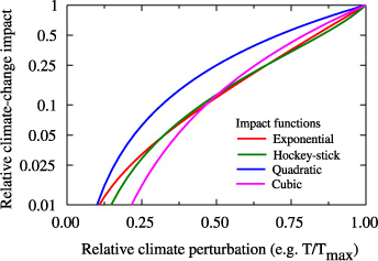
Figure 1. Quantification of climate-change impacts as a function of relative climate perturbations. This is illustrated for the exponential relationship used here, the 'hockey-stick' function of Hammitt et al (1996) and quadratic and cubic impact functions. It is shown for different relative climate perturbations, such as temperature changes, relative to the maximum perturbations anticipated over the next 100 years.
Download figure:
Standard image High-resolution imageEconomic analyses tend to employ quadratic or cubic responses function (e.g. Nordhaus 1994, Hammitt et al 1996, Roughgarden and Schneider 1999, Tol 2012), but there is concern that these functions that are based only on readily quantifiable impacts may give insufficient weight to the small probability of extremely severe impacts (e.g. Weitzman 2012, 2013, Lemoine and McJeon 2013). A response function that includes these extreme impacts would increase much more sharply than quadratic or cubic response functions (e.g. Weitzman 2012).
The relationship used here uses an exponential increase in impacts with increasing perturbations to capture the sharply increasing damages with larger temperature increases (as shown by Hammitt et al 1996 and Weitzman 2012). Warming by 3/4 of the expected maximum warming, for example, would have about 10 times the impact as warming by only 1/4 of maximum warming. The graph also shows the often-used power relationships (e.g. Hammitt et al 1996, Boucher 2012), shown here with powers of 2 (quadratic) and 3 (cubic), and a more extreme impacts function (hockey-stick function) presented by Hammitt et al (1996). Compared to the power functions, the exponential relationship calculates relatively modest impacts for moderate climate perturbations that increase more sharply for more extreme climate perturbations. It is thus very similar to the 'hockey-stick' relationship of Hammitt et al (1996).
2.5. Discount factors
Should near-term impacts be treated as more important than more distant impacts? If one applies discount rates of 4%, for example, it would render impacts occurring in just 17 years as being only half as important as impacts occurring immediately. The choice of discount rates is hence one of the most critical components of any impact analysis, and the influential Stern report (Stern 2006) derived a fairly bleak outlook on the seriousness of climate change, largely due to using an unusually low discount rate of 1.4%.
While the use of large discount rates is warranted in purely economic analyses, it is questionable in environmental assessments as it essentially treats the lives and livelihood of our children and grandchildren as less important than our own, which is hard to justify ethically (e.g. Schelling 1995, Sterner and Persson 2008). On the other hand, using a 0 discount rate would treat impacts in perpetuity as equally important as short-term impacts. This raises at least the practical problem that it becomes increasingly difficult to predict events and their significance into the more distant future.
The calculation of GWPs essentially uses 0 discount rates, but ignores impacts beyond the end of the assessment period (Tanaka et al 2010). This avoids a preferential emphasis on the impacts on one generation over another, yet avoids the unmanageable requirement of having to assess impacts in perpetuity. This approach is also used here for calculating CCIPs.
3. Calculation methods
3.1. Quantifying climate-change impact potentials
To quantify the three different kinds of impacts, it is necessary to first calculate the climate perturbations underlying them. The perturbation Py, T in year y, related to direct-temperature impacts, is simply calculated as:

where Ty and Tp are the temperatures in year y and pre-industrially. The temperature in 1900 is taken as the pre-industrial temperature.
The rate of temperature change, Py, Δ , is calculated as the temperature increase over a specified time frame:

where d is the length of the calculation interval, set here to 100 years. Shorter calculation intervals could be used, in principle, but extra emission units would then affect both the starting and end points for calculating rates of change, leading to complex and sometimes counter-intuitive consequences. The choice of 100 years is further discussed below.
The cumulative temperature perturbation, Py, Σ , is calculated as the sum of temperatures above pre-industrial temperatures:
where Ti is the temperature in every year i from pre-industrial times to the year y.
All three perturbations are then normalized to calculate relative perturbations, Q, as:


where the P-terms are the calculated perturbations under a chosen emissions pathway, and the max-terms are the maximum perturbations calculated under RCP6 over the next 100 years. With this normalization, each kind of climate impact can be treated mathematically the same.
Impacts, I, are then derived from relative perturbations as:


where s is a severity term that describes the relationship between perturbations and impacts (figure 1). The work presented here uses s = 4 (as discussed in section 2.4 above).
Temperatures from 1900 to 2010 were based on the HadCRUT4 data set of Jones et al (2012). They were used to set initial temperatures for calculating rates of warming and cumulative warming up to 2010. Temperatures beyond 2010 were added to base temperatures and together determined respective perturbations over the next 100 years.
The relevant impacts were then calculated using equation (4), and summed over 100 years. To calculate CCIPs, these calculation steps were followed four times. The first set of calculations was based on RCP6 and was only used to derive max(PRCP6) which was needed for subsequent normalizations. This normalization made it possible to assign each kind of impact equal importance at their highest perturbations over the next 100 years under RCP6.
The second set of calculations used a chosen emission pathway, RCP6, or a different one as specified below, to calculate background gas concentrations and perturbations. The final two sets of calculations used the same chosen emission pathway and added either 1 tonne of CO2 or of a different gas. The calculations then derived marginal extra impacts of extra emission units under the three different kinds of impacts. CCIPs of each gas were then calculated as the ratios of marginal impacts of different gases relative to those of CO2.
These calculations aim to estimate impacts over the coming 100 years, and how those impacts might be modified through pulse emissions of different GHGs. They use the best estimates of relevant background conditions based on emerging science and updated emission scenarios. These calculations would need to be repeated every few years with new scientific understanding and newer emission projections to provide updated guidance of the importance of different GHG over the next 100-year period.
3.2. Calculating radiative forcing and temperature changes
The calculations of radiative forcing and temperature followed the approach of Kirschbaum et al (2013), including the carbon cycle based on the Bern model and radiative forcing calculations provided by the IPCC. Calculations also included the replacement of a molecule of CO2 by CH4 in the biogenic production of CH4, and its partial conversion back to CO2 when CH4 was oxidized (Boucher et al 2009). Global temperature calculations included a term for the thermal inertia of the climate system. Full calculation details are given in the supplemental information (available at stacks.iop.org/ERL/9/034014/mmedia).
4. Results
4.1. Impacts under business-as-usual concentrations
A quantification of the marginal impact of additional units of each gas must be based on background conditions that include quantification of the impacts that are expected to occur without those additional emission units. Figure 2 shows the relative perturbations underlying the three kinds of impacts and resultant calculated climate-change impacts.

Figure 2. Relative climate perturbations (a) and resultant impacts (b) for the three kinds of impacts calculated under RCP6. T refers to direct-temperature impacts, Δ to rate-of-warming impacts, and Σ to cumulative-warming impacts. All values are expressed relative to their calculated maxima over the next 100 years. Maximum perturbations to 2109 under RCP6 were 2.6 °C, 0.016 °C yr−1 and 206 °C yr, respectively.
Download figure:
Standard image High-resolution imageUnder RCP6, direct and cumulative-warming impacts continue to increase throughout the 21st century, with greatest impacts reached by 2109. Rate-of-warming impacts reach their maximum by about 2080 and then start to fall slightly (figure 2(a)). While the underlying climate perturbations increase fairly linearly over the next 100 years, this leads to sharply increasing impacts towards the end of the assessment period (figure 2(b)). This pattern is most pronounced for cumulative-warming impacts. The irregular pattern in calculated rates of warming is related to the unevenness in the observed temperature records up to 2010 as rates of warming are calculated from the temperature difference over the preceding 100 years.
4.2. Physico-chemical effects of extra GHG emissions
To calculate the marginal impact of pulse emissions of extra GHG units, it is necessary to first establish their physico-chemical consequences. Concentration increases are greatest immediately after the emission of extra units. They then decrease exponentially for CH4 (figure 3(b)) and N2O (figure 3(c)). CO2 concentrations also decrease but follow a more complex pattern (figure 3(a)). For CH4, the decrease is quite rapid, with a time constant of 12 years, but is more prolonged for N2O, with a time constant of 120 years.
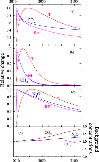
Figure 3. Calculated increases in the concentrations of CO2 (a), CH4 (b) and N2O (c) due to pulse emissions of each gas in 2010 and the resultant radiative forcing and temperature increases. Also shown are relative changes in background gas concentrations according to RCP6 (d). All values in (a)–(c) are expressed relative to their highest values over the next 100 years, and concentrations in (d) are relative to 2010 concentrations.
Download figure:
Standard image High-resolution imageThese concentration changes exert radiative forcing. It is also highest immediately after the emission of each gas and decreases thereafter. It decreases proportionately faster than the concentration decrease because of increasing saturation of the relevant infrared absorption bands. This is most pronounced for CO2 (figure 3(a)), for which RCP6 projects large concentration increases (figure 3(d)), which makes the remaining CO2 molecules from 2010 pulse emissions progressively less effective (e.g. Reisinger et al 2011). For N2O, RCP6 projects only moderate concentration increases. The infrared absorption bands of N2O are also less saturated than for CO2 so that the effectiveness of any remaining molecules remains high. RCP6 projects little change in the CH4 concentration. Radiative forcing then drives temperature changes (figure 3) that lag radiative forcing by 15–20 years due to the thermal inertia of the climate system.
4.3. Marginal impacts of extra emission units
From the information in figures 2 and 3, one can calculate marginal increases in impacts due to a 2010 pulse emission of each gas (figure 4). Extra units of CO2 emitted in 2010 cause the largest temperature increase in about 2025 (figure 3(a)). Base temperatures, however, are still fairly mild in 2025 (figure 2(a)) so that the extra warming at that time increases direct-temperature impacts only moderately (figure 4(a)). Even though the extra warming from CO2 added in 2010 diminishes over time (figure 3(a)), it adds to increasing base temperatures (figure 2(a)) to cause increasing ultimate impacts (figure 4(a)). This pattern is strongest for cumulative-warming impacts. The patterns for N2O (figure 4(c)) are similar to those for CO2 because the longevity of N2O in the atmosphere is similar to that of CO2.

Figure 4. Change in the three kinds of impacts due to the addition of one unit of CO2 (a), biogenic CH4 (b) and N2O (c) in 2010. Symbols as for figure 2. All numbers are normalized to the highest marginal impacts calculated over the next 100 years.
Download figure:
Standard image High-resolution imageCH4 emitted in 2010, however, modifies direct-temperature impacts only over the first few decades after its emission (figure 3(b)). While later warming could potentially have greater impacts, the residual warming several decades after its emission becomes so small to have very little effect. For cumulative-warming impacts, however, the greatest marginal impact of CH4 additions also occurs at the end of the assessment period. Even though CH4 emissions exert their warming early in the 21st century, that warming is effectively remembered in the cumulative temperature record and leads to the largest ultimate impact when it combines with large cumulative-warming base impacts (figure 4(b)).
For rate-of-warming impacts and direct-temperature impacts, there are distinctly different patterns for the different gases that are principally related to the longevity of the gases in the atmosphere. For cumulative-warming impacts, however, the patterns are similar for all gases, with the marginal impact from a 2010 pulse emission being muted for the first 50–80 years and then increasing sharply over the remainder of the 100-year assessment period. This is because cumulative warming can be increased in much the same way for contributions made earlier as from on-going warming. Even though different gases make their additions to cumulative warming at different times, that increased perturbation has the largest impact when it adds to large base values (see figure 2(a)) so that for all gases, the largest marginal impacts occur at the end of the 100-year assessment period (figure 4).
4.4. Climate-change impact potentials
Marginal impacts can then be summed over the 100 years after the pulse emission of each gas and expressed relative to CO2 (table 1). Under RCP6, CCIPs for biogenic and fossil CH4 are 20 and 23, respectively, compared to a 100-year GWP of 25. These lower values are due to the much lower direct-temperature and rate-of-warming impacts. Peak warming from CH4 emissions in 2010 occurs at a time when background temperature increases are still fairly mild so that the extra warming from CH4 (figure 4(b)) causes less severe impacts than the warming from CO2 (figure 4(a)) that is still strong many decades later when it combines with higher background temperatures to cause more severe additional impacts.
Table 1. Cumulative radiative forcing, the three kinds of impacts calculated separately and combined to calculate CCIPs over 100 years. Calculations are done under constant 2010 GHG concentrations, and under four different RCPs. All numbers are expressed relative to CO2. Calculations are done separately for biogenic (B) and fossil-derived (F) CH4. CCIPs are calculated as the average of the three individually calculated kinds of impacts. Calculations under RCP6 are shown in bold as the reference condition used here. Constant 2010 concentrations were taken to be 387, 1.767 and 0.322 ppmv for CO2, CH4 and N2O, respectively. Numbers for cumulative radiative forcing are given only for comparison. Currently used 100-year GWPs are 25 for CH4 and 298 for N2O.
| Cumulative radiative forcing | Direct-temperature impacts | Rate-of-warming impacts | Cumulative-warming impacts | CCIPs | ||
|---|---|---|---|---|---|---|
| CH4 (B) | Const | 22 | 23 | 34 | 32 | 29 |
| CH4 (F) | 24 | 25 | 36 | 34 | 32 | |
| N2O | 282 | 285 | 285 | 288 | 286 | |
| CH4 (B) | RCP3 | 24 | 24 | 32 | 35 | 30 |
| CH4 (F) | 27 | 27 | 35 | 37 | 33 | |
| N2O | 306 | 313 | 313 | 313 | 313 | |
| CH4 (B) | RCP4.5 | 26 | 16 | 19 | 34 | 23 |
| CH4 (F) | 29 | 19 | 22 | 37 | 26 | |
| N2O | 331 | 341 | 342 | 328 | 337 | |
| CH4 (B) | RCP6 | 27 | 12 | 13 | 34 | 20 |
| CH4 (F) | 30 | 15 | 16 | 37 | 23 | |
| N2 O | 338 | 359 | 356 | 329 | 348 | |
| CH4 (B) | RCP8.5 | 29 | 5.0 | 3.9 | 34 | 14 |
| CH4 (F) | 32 | 7.8 | 6.7 | 37 | 17 | |
| N2O | 365 | 437 | 438 | 351 | 408 |
In contrast, cumulative-warming impacts under RCP6 are 34 and 37 (for biogenic and fossil CH4), which are greater than the corresponding values for cumulative radiative forcing. The earlier radiative forcing from CH4 ensures that all radiative forcing leads to warming within the assessment period. For CO2 and N2O, on the other hand, radiative forcing overestimates their warming impact because of the thermal inertia of the climate system. Some of the radiative forcing exerted towards the end of the 100-year assessment period only leads to warming after the end of the assessment period providing relatively more cumulative radiative forcing than cumulative warming.
Fossil-fuel-derived CH4 has higher CCIPs than biogenic CH4 by about three units. Biogenic CH4 production means that a molecule of carbon is converted to CH4, which lowers the atmospheric CO2 concentration and thereby reduces its overall climatic impact. After it has been oxidized, any CH4, however, continues its radiative forcing as CO2, which increases its overall impact (Boucher et al 2009), with the same effect for both fossil and biogenic CH4.
CCIPs of CH4 become progressively smaller when they are calculated under higher concentration pathways (table 1). This is caused by much higher impact damages being reached under higher concentration pathways so that the earlier warming contribution of CH4 relative to CO2 becomes increasingly less important. This affects direct-temperature impacts and rate-of-warming impacts, whereas cumulative temperature impacts remain similar under the different RCPs.
For N2O, the CCIP is greater than the 100-year GWP (348 versus 298 under RCP6). This is mainly due to the reducing effectiveness of infrared absorption of extra CO2 under increasing background concentrations, which increases the relative importance of the emission of other gases. This interaction with base-level gas concentrations is not included in GWPs as they are calculated under constant background gas concentrations.
4.5. The importance of climate-change severity
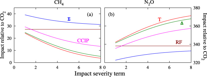
The relative importance of different gases also depends strongly on the underlying climate-change severity term (figure 5). With increases in the severity term, the importance of short-lived CH4 decreases considerably (figure 5(b)), whereas the importance of N2O increases slightly (figure 5(a)). This is because the greatest temperature and rate of change perturbations are projected to occur at the end of the assessment period when CH4 adds little to those perturbations, while N2O adds even more than CO2. As the climate-change severity term increases, it progressively increases the importance of impacts at these later periods and thereby greatly reduces the importance of CH4.
Figure 5. Dependence of cumulative radiative forcing (RF) and CCIPs and its components on the climate-impact severity terms for biogenic CH4 (a) and N2O (b). T refers to direct-temperature impacts, Δ to rate-of-warming impacts, Σ to cumulative-warming impacts, RF to radiative forcing and CCIP to the derived combined index.
Download figure:
Standard image High-resolution image
5. Discussion
In this work, climate-change impact potentials are presented as an alternative metric for comparing different GHGs. Why use a new metric? The ultimate aim of climate-change mitigation is to avert adverse climate-change impacts. Hence, there is an obvious logic for policy setting to start with a clear definition of the different kinds of climatic impacts that are to be avoided. Climate-change metrics are needed to support that climate-change policy with the same definition and quantification of climate-change impacts so that the effects of different GHGs can be compared. Mitigation efforts can then be targeted at the gases through which mitigation efforts can be achieved most cost-effectively.
The key aim of metrics should be the quantification of the marginal impact of pulse emissions of extra GHG units. CCIPs aim to provide that measure. They aim to achieve that by combining simple calculations of the relevant physics and atmospheric chemistry with an assessment of the key impacts on nature and society. This full assessment is needed to underpin the development of the most cost-effective mitigation strategies.
The calculation of CCIPs begins with setting the most likely background conditions with respect to gas concentrations and background temperatures in order to quantify the marginal impact of an extra emission unit of a GHG. The use of CCIPs thus requires a periodic re-evaluation of background conditions to devise new optimal mitigation strategies. It is necessary for mitigation efforts to be continuously refocused to achieve the most cost-effective climate-change impact amelioration (Johansson et al 2006). This is first because the relative importance of extra GHG units diminishes with an increase in their own background concentrations because of increasing saturation of the relevant infrared absorption bands. Conversely, the extra warming caused by additional emission units has a greater impact when background temperatures are already higher as it can contribute towards raising temperatures into an increasingly dangerous range. The marginal impact of extra emission units can, therefore, only be quantified under a specified emissions pathway and time horizon.
Along the chain of causality from greenhouse gas emissions to ultimate climate-change impacts, the relevance of respective metrics increases but the uncertainty associated with their calculation increases as well (e.g., Fuglestvedt et al 2003). This relates to scientific uncertainty, the value judgements needed about the relative importance of different impacts, and the ethical considerations of accounting for impacts occurring at different times. GWPs are at one extreme of this continuum, requiring a minimum of assumptions in their calculation, but they only quantify a precursor of ultimate impacts. CCIPs try to go several steps further by quantifying specific climate perturbations that are more directly related to different kinds of climate-change impacts. The functions used to calculate CCIPs still retain simplicity and transparency.
The use of CCIPs instead of 100-year GWPs would reduce the short-term emphasis on CH4 as CH4 emitted in 2010 will have disappeared from the atmosphere by the time the most damaging temperatures or rates of warming will be reached. This conclusion is similar to that reached by studies based on GTP calculations (e.g. Shine et al 2007). However, even CH4 contributes to cumulative-warming impacts. Using CCIPs would thus make CH4 less important without rendering it irrelevant. Over time, and if future GHG emissions remain high, CH4 is likely to become more important as the time of emission gets closer to the times when the most severe impacts may be anticipated (Shine et al 2007, Smith et al 2012). CH4 would then increasingly contribute not only to cumulative-warming impacts but also to direct-temperature and rate-of-warming impacts. CCIPs would need to be recalculated periodically in line with continuously changing expectations of the future.
CCIPs also change with background conditions, and it is considered likely that CCIPs calculated under RCP6 are the most relevant. Recent concentration trends, even during times of global economic crisis (e.g. Peters et al 2013), point towards higher concentration pathways. The limited willingness of the international community to seriously address climate change also suggests that higher concentration pathways will be more likely. RCP6 was therefore used here as the most likely background condition from which to assess the marginal impacts of the emission of extra GHG units.
The derivation of CCIPs explicitly defined and quantified three distinct kinds of impacts. They were all related to temperature as even climate impacts such as flooding that may be more directly related to rainfall intensity can be related to temperature-based perturbations as the underlying climatic driver. One impact that cannot be related to temperature is the direct impact of elevated CO2 itself. Increasing CO2 leads to ocean acidification (e.g. Kiessling and Simpson 2011) and shifts the ecological balance between plant species, especially benefiting C3 plants at the expense of C4 plants (e.g. Galy et al 2008). On the other hand, increasing CO2 is beneficial through increasing biological productivity and may partly negate the pressures on food production from increasing temperatures and precipitation changes (e.g. Jaggard et al 2010). With these divergent impacts its overall net impact remains uncertain, and may even be regarded as either positive or negative, and it was, therefore, not included in the CCIP calculations.
Another critically important factor is the steepness of the relationship between underlying climate perturbations and their resultant impact (figures 1, 5). The more steeply impacts increase with increasing perturbation, the more it shifts the importance of extra warming to the times when impacts are already high. With a less steep impact curve, warming at times with lower background temperatures also makes significant contributions towards the overall impact load. The present work used a response function similar to the 'hockey-stick' function first presented by Hammitt et al (1996). This steep response curve emphasizes the contribution of different gases at the times of highest impacts while reducing the importance of their contributions at times of lower background impacts. It thus reduces the importance of short-lived gases such as CH4.
It is also important over what time interval relevant rate-of-warming impacts are calculated. The present work used an assessment period of 100 years and calculated the rate of warming from the temperature increase over the preceding 100 years. With these assumptions, the starting temperatures are always part of the immutable past and extra emissions affect only the end-point temperatures. However, a calculation interval of 100 years may be regarded as too long (e.g. Peck and Teisberg 1994) and a shorter interval might be seen as more appropriate.
Shortening the calculation interval to less than 100 years, however, creates complex interactions because extra emission units then affect both the starting and end point for calculating the rate of warming, and results can become complex and counter-intuitive. For instance, if rates of warming were calculated over 50 years, extra methane emissions would paradoxically reduce the sum of calculated rate-of-warming impacts. How does that occur? While extra methane would increase temperatures over a few decades after its emission, it would increase the short-term rate of warming (calculated from, say, 1970–2020), but it would reduce the rate of warming calculated from 2020 to 2070. Since higher rates of warming are anticipated later during the 21st century (see figure 2), the gains from decreasing the more damaging rates of warming at the later time would be greater than the harm from marginally worsening the milder rates-of-warming impacts in the shorter term.
Whether extra emissions would be considered to do ultimate harm or good would thus depend on the timing of those respective increased and decreased perturbations relative to the base perturbations and the length of period that is assessed as most appropriate for assessing rate-of-warming impacts. Exploring these complex interactions is beyond the scope of the present paper, and the present work had to restrict itself to the simpler case of calculating rates-of-warming impacts by the temperature change over 100 years.
The calculation of CCIPs cannot be based purely on objective science, but has to combine scientific insights with value judgements and assumptions about future background conditions. They relate to the steepness of the impacts function, the choice of background scenario, the inclusion or exclusion of time discounting, the length of assessment horizon, the relative weighting assigned to the different kinds of impacts, the length of the time period for quantifying the rate of change and others. These choices all have a bearing on calculated CCIPs. It may be seen as unfortunate that CCIPs cannot be developed without recourse to a number of key assumptions. However, society makes these assumptions implicitly whenever it decides on adopting any policies related to climate change. The process that is followed formally and explicitly in this paper is similar to the process followed implicitly in all discussions of the importance of climate change, and that has led to the current level of concern and partial willingness to pursue mitigative measures.
Various possible metrics to account for different GHG emissions have been proposed in the past (Ekholm et al 2013). They fall under three broad categories: (1) using measures of cumulative radiative forcing, such as for GWPs; (2) rate of warming, like that explored by Peck and Teisberg (1994); and (3) a number of proposals that are predicated on impacts related directly to elevated temperature, such as the Global Damage Potential (Kandlikar 1996, Hammitt et al 1996, see also Boucher 2012), and the Global Temperature Change Potential, GTP, (Shine et al 2005, 2007). The present work is the first to derive a metric explicitly based on all three kinds of impacts.
Metrics may also restrict themselves to the use of physico-chemical quantities, such as the GWP or the GTP, or employ detailed economic analyses to derive ultimate cost or damage functions (e.g. Kandlikar 1996, Manne and Richels 2001). Including explicit models to calculate damages aims to get closer to an explicit calculation of the ultimate impacts that matter, but it greatly reduces the transparency of resultant metrics (Johansson 2012). It also tends to bias analyses towards those aspects that can be quantified more readily, such as economic impacts, while other impacts, such as the perceived loss from the extinction of species, or the damage from low-probability, but high impact, events tend to be ignored (e.g. Weitzman 2012). The present work restricts itself to using simple models for calculating physico-chemical processes that allowed a number of critical assumptions to remain explicit and transparent. It thereby aims to retain the transparency needed for adoption in international policy or research applications.
6. Conclusions
Global Warming Potentials calculated over 100 years are the current default metric to compare different GHGs. They have become the default metric despite the recognition that they are not directly related to the ultimate climate-change impacts that society is trying to avert. To achieve mitigation objectives most cost-effectively, and to be able to target an optimal mix of GHGs, requires a clearer definition of what is to be avoided. This, in turn, necessitates a more complex analysis than provided by the use of GWPs.
Over the years, there have been several proposals of alternative accounting metrics. A key difference between these different metrics lies in their damage functions that may be related directly to elevated temperature (e.g. Kandlikar 1996, Shine et al 2005, 2007), or to the rate of warming (Peck and Teisberg 1994), or to a measure of cumulative radiative forcing (as for GWPs). However, no previously proposed metric explicitly included all three different kinds of climate perturbations that all contribute towards overall impacts (e.g. Fuglestvedt et al 2003, Brandão et al 2013). Instead, previous work derived respective metrics based on only one of these kinds of impacts and thus implicitly negated the importance of the other kinds of impacts. CCIPs are the first attempt to explicitly develop a metric that is based on all three kinds of impacts.
Climate change continues to be a significant threat for the future of humanity, and mitigation is needed to avert those threats as much as possible. The global community, however, is showing only a limited willingness to allocate sufficient resources to avert serious long-term impacts. The development of CCIPs aims to assist in using those limited resources as cost-effectively as possible.
Acknowledgments
I would like to thank colleagues at Landcare Research, especially Phil Cowan, for discussions underlying the development of the proposed methodology, and Robbie Andrew, Anne Austin, Annette Cowie, Édouard Périé and Katsumasa Tanaka and anonymous reviewers for many useful and insightful comments on the manuscript.