

Abstract
In April 2015, the Governor of California mandated a 25% statewide reduction in water consumption (relative to 2013 levels) by urban water suppliers. The more than 400 public water agencies affected by the regulation were also required to report monthly progress towards the conservation goal to the State Water Resources Control Board. This paper uses the reported data to assess how the water utilities have responded to this mandate and to estimate the electricity savings and greenhouse gas (GHG) emissions reductions associated with reduced operation of urban water infrastructure systems. The results show that California succeeded in saving 524 000 million gallons (MG) of water (a 24.5% decrease relative to the 2013 baseline) over the mandate period, which translates into 1830 GWh total electricity savings, and a GHG emissions reduction of 521 000 metric tonnes of carbon dioxide equivalents (MT CO2e). For comparison, the total electricity savings linked to water conservation are approximately 11% greater than the savings achieved by the investor-owned electricity utilities' efficiency programs for roughly the same time period, and the GHG savings represent the equivalent of taking about 111 000 cars off the road for a year. These indirect, large-scale electricity and GHG savings were achieved at costs that were competitive with existing programs that target electricity and GHG savings directly and independently. Finally, given the breadth of the results produced, we built a companion website, called 'H2Open' (https://cwee.shinyapps.io/greengov/), to this research effort that allows users to view and explore the data and results across scales, from individual water utilities to the statewide summary.
Export citation and abstract BibTeX RIS

Original content from this work may be used under the terms of the Creative Commons Attribution 3.0 licence.
Any further distribution of this work must maintain attribution to the author(s) and the title of the work, journal citation and DOI.
1. Introduction
In 2015, California confronted its fourth year of drought, facing a 48% deficit (2 835 000 million gallons, MG) in surface water resources below baseline conditions (Howitt et al 2015). The drought led to the fallowing of 542 000 acres of land, total economic costs of $2.74 billion, and the loss of approximately 21 000 jobs (Howitt et al 2015). In response to the dire conditions, on April 1, 2015, Governor Jerry Brown enacted Executive Order B-29-15 that sought to mobilize a comprehensive response to the drought, including a mandate to reduce urban water consumption for the first time in state history (Brown 2015).
The mandate authorized the State Water Resources Control Board (SWRCB) to enforce a 25% reduction (on average) in urban water consumption relative to 2013 baseline levels and to impose a requirement on urban water suppliers to report their monthly progress towards this goal to the SWRCB (Brown 2015). Recognizing that Californian water agencies vary significantly in their per capita consumption, the Executive Order allowed the SWRCB to set restrictions proportional to the per capita consumption at each individual water agency (Brown 2015). In response, the SWRCB approved an Emergency Regulation (Resolution No. 2015−0032) that established conservation tiers with varying conservation targets, ranging from 4%–36% relative to the 2013 baseline (SWRCB 2015).
In 2013, total urban water consumption in California was approximately 2 140 000 MG. Thus, an average 25% reduction across all regulated water agencies represented a significant statewide decrease in consumption of 535 000 MG. A reduction in water consumption of this magnitude has implications that stretch beyond the water sector, and this paper explores the potential impacts of reduced urban water deliveries in terms of reduced electricity consumption and GHG emissions associated with reduced water infrastructure operations across the State.
It is well-established that the water and energy utility sectors are interrelated and interdependent (Stanford 2013). Water is required to produce energy across nearly all fuels and electricity generation technologies (Macknick et al 2011, Gleick 1994), and energy is required to treat and convey both water and wastewater (Young 2015, Gleick 1994). This overall relationship, the water-energy nexus, has been explored and evaluated at multiple scales, from the urban (Nair et al 2014) to the national (Sanders and Webber 2012, Macknick et al 2012) to the global scale (Holland et al 2015, Spang et al 2014).
This paper explores the energy-for-water side of the nexus, which has been an area of active research for well over a decade in California (Spang and Loge 2015, Bennett et al 2010, Klein et al 2005, Wilkinson 2000). California represents an intriguing case study for the topic because of the large water conveyance systems (with attendant high energy demands for pumping) that deliver water from the relatively wetter northern areas of the state to the drier and populated southern region (including the large metropolitan areas of Los Angeles and San Diego). The energy demand from these large-scale conveyance systems in combination with water and wastewater utility energy use for treatment and distribution, and end-user water consumption for heating and additional pumping and treatment, is estimated to represent approximately 19% of total electricity demand and 32% of total non-power plant natural gas demand statewide (Klein et al 2005).
Our analysis focuses specifically on the electricity savings associated with large-scale water conservation, and not natural gas, because the vast majority of energy embedded in water at the point of delivery is electricity consumed by water pumping and treatment infrastructure (Klein et al 2005). Conversely, the majority of natural gas consumed in the water system is for water heating on the consumer side of the water meter (Klein et al 2005). This makes it difficult, if not impossible, to attribute any natural gas savings to externally observable reductions in water consumption, and therefore is outside the scope of this paper.
Beyond the direct linkage between water use and electricity consumption, it is a short leap to consider the GHGs associated with the electricity portion of the nexus. Emissions factors for the regional grid can be applied directly to convert estimated electricity use to GHG emissions. A number of studies in the literature have explicitly addressed the water–energy–GHG connection, ranging from more generalized approaches for calculating and reporting GHG emissions in the urban water sector (Oppenheimer et al 2014, Nair et al 2014) to site-specific energy and GHG intensity metrics for individual regional and urban water systems (Fang et al 2015, Venkatesh et al 2014).
This study builds on this previous work by producing an estimate of the statewide electricity and GHG savings associated with the drought-based urban water conservation mandate in California. In addition, we explore the relative costs to securing the electricity and GHG savings through water conservation relative to traditional programs targeting these savings directly. Finally, given the breadth of the results produced, we built a companion website, called 'H2Open' (https://cwee.shinyapps.io/greengov/), to this research effort that allows users to view and explore the data and results across scales, from individual water utilities to the statewide summary.
2. Methodology
To estimate the water, energy, and GHG savings achieved for the duration of the Governor's urban water conservation Executive Order B-29-15, we collected and consolidated a range of publicly available data relevant to the analysis. In sequential order, we estimated total water savings for each water agency reporting to the SWRCB; the associated energy savings via spatially resolved estimates of the energy intensity of water supplies by hydrologic region; and finally, the linked GHG emissions reduction using the emissions factor for the California regional electricity grid. Finally, we made comparisons of the cost of securing these savings through water conservation to the costs of existing programs that specifically target electricity or GHG savings.

Figure 1. Water consumption by urban water supplier service area (a), and IOU energy intensity (b) and total energy intensity (c) by California's hydrologic regions. 'CC' = Central Coast, 'CR' = Colorado River, 'NC' = North Coast, 'NL' = North Lahontan, 'SR' = Sacramento River, 'SF' = San Francisco, 'SJ' = San Joaquin River, 'SC' = South Coast, 'SL' = South Lahontan, and 'TL' = Tulare Lake.
Download figure:
Standard image High-resolution image2.1. Water conservation
Our estimation of the total water saved for the duration of conservation mandate period (June 2015–May 2016) was derived from monthly water consumption values reported directly by urban water agencies to the SWRCB. The SWRCB publishes this data publicly through their online 'Water Conservation Portal' (SWRCB 2016). The monthly consumption data for the mandate period was compared directly to monthly consumption values for 2013 (the baseline consumption year as specified by Executive Order B-29-15). We collected and analyzed the data at the scale of each individual urban water agency that reported to the SWRCB (figure 1(a), detailed data available in table 1 of the supplementary information available at stacks.iop.org/ERL/13/014016/mmedia). We then consolidated all of these reports up to the statewide scale to obtain an estimate of total statewide water conservation achieved.
Table 1. Total GHG emissions savings by hydrologic region.
| Hydrologic region | MT CO2e saved |
|---|---|
| Central Coast | 10 210 |
| Colorado River | 4870 |
| North Coast | 1310 |
| North Lahontan | 380 |
| Sacramento River | 15 150 |
| San Francisco Bay | 50 400 |
| San Joaquin | 9160 |
| South Coast | 401 790 |
| South Lahontan | 12 430 |
| Tulare Lake | 15 810 |
As shown in figure 1(a), the urban water agency service territories represent a relatively small geographic portion of the state. This spatial distribution is a function of the definition of urban water agencies, which are defined as providing municipal water services to more than 3000 customers, or more than 3000 acre-feet annually (State of California 2010). Thus, the locations of urban water service territories coincide with the medium to high population centers in the state, and the remaining area (the gray area in figure 1(a)) represents a mixture of rural, agricultural, and natural land areas.
2.2. Energy and GHG savings from water conservation
To estimate the energy savings resulting from reduced water deliveries we applied spatially disaggregated estimates of energy intensity (the energy required to deliver a unit of water to the end-user) for the water supply portfolios associated with the ten hydrologic regions of California (figures 1(b) and (c)). We use two estimates for energy intensity in this study: 'Total' and 'IOU'. Total energy intensity refers to the total electricity consumption for water services provision, regardless of the institution that generated the electricity, whether an investor-owned utility (IOU) or a public provider. IOU energy intensity refers only to the electricity consumed by the water infrastructure that was generated by an IOU. Differentiating between the energy providers that power the statewide water infrastructure systems is an important policy distinction because the California Public Utilities Commission (CPUC) only has regulatory authority over the IOUs. This authority includes regulation of the more than $1 billion per year allocated to IOU energy efficiency programs (CPUC 2016b). Thus, estimating specifically the IOU energy savings linked to water conservation is critical component for enabling the CPUC to direct energy efficiency funds towards water conservation programs that jointly demonstrate water and energy savings.
The total and IOU energy intensity estimates come from a report sponsored by the CPUC (Navigant 2015a, 2015b). These estimates were produced by taking the weighted average of the energy intensities for the average water supply and technology mix for each hydrologic zone. The energy intensity estimates were collected from a breadth of existing literature and consolidated into four main components of water infrastructure systems (extraction and conveyance, water treatment, distribution, and wastewater systems). The energy intensity of extraction and conveyance varies significantly by hydrologic zone given the large-scale water transfer systems that exist within the state, while the energy intensity of water and wastewater treatment systems vary significantly by the type of technology deployed and the quality of the water or wastewater source (Navigant 2015b). Meanwhile, the energy intensity of distributing water within the utility service territories varies significantly based on the topography of the local water systems, and this component was addressed by categorizing each hydrologic zone as either 'flat', 'moderate', or 'hilly' and assigning a related energy intensity to each category (Navigant 2015b). It is worth noting that the spatial heterogeneity of energy intensity can be significantly more nuanced between (and even within) water agencies than is provided by estimates at the scale of the hydrologic region (Spang and Loge 2015). However, given that high-resolution estimates for energy intensity are not currently available statewide, we had to rely on the more aggregated estimates from the CPUC report for this analysis.
The CPUC partitions energy intensity into two values: 'outdoor' and 'indoor'. Outdoor energy intensity reflects the energy intensity of the potable water system (e.g. the energy expended to extract and convey, treat, and distribute water). Indoor energy intensity reflects the energy expended in the potable water system as well as the wastewater system (e.g. the energy expended to collect and treat wastewater). In California, the vast majority of service connections to the potable water system have meters, but very few, if any, have wastewater meters. Hence, for our study, we chose to use the outdoor energy intensity to produce a lower bound estimate of statewide energy savings achieved from the water conservation mandate.
Once we had total and IOU energy intensity estimates for each hydrologic region, we associated the location of every urban water agency (GreenGov 2016) reporting to SWRCB to its hydrologic region using GIS. This allowed us to assign unique regional energy intensity values (total and IOU) to each of the 408 urban water agencies included in the study (table 1, supplementary information).
The energy intensity values were then applied as a conversion factor to the total observed water savings over the mandate period to estimate the associated electricity savings for each reporting water agency individually (equation 1) and in total across the state (equation 2). We calculated separate estimates for total and IOU electricity savings using the differentiated energy intensity factors as shown in figure 1.

where,
ESi = electricity savings estimated from water conservation at water agency i in kilowatt-hours (kWh).
WSi = water savings reported by water agency i in million gallons (MG).
EIi = energy intensity estimate (either total or IOU, in kWh MG−1) for water agency i.
ESCA = statewide electricity savings (either total or IOU) estimated from water conservation for all (n) reporting water agencies in California, in MWh.
To get a sense of the overall scale of the electricity savings achieved during the urban water conservation mandate period (June 2015–May 2016), we compared our estimates to the total first-year electricity savings from the energy efficiency (EE) programs funded by the energy IOUs over roughly the same time period (July 2015–June 2016). The program investments and estimated savings are published through the CPUC's Energy Efficiency Data Portal (CPUC 2016a). Example EE investments include programs that target indoor and outdoor lighting; whole building improvements; and heating, ventilation and air conditioning (HVAC) systems (see figure 4 for full list of major end-use categories).
The estimated total electricity savings were converted to GHG emissions reductions using a 2015 emissions factor estimate for the California electricity mix. The GHG intensity factor (0.285 metric tonnes (MT) CO2e MWh−1) was derived from in-state generation and imported electricity data from the California Energy Commission (CEC) (CEC 2017), and the associated GHG emissions data from the California Air Resources Board (CARB) (CARB 2017). While it would have been preferable to use GHG emissions factors specific to sub-regional electricity providers in the state, the interconnected nature of the California water system limits our ability to disaggregate the embedded energy of water by specific energy provider. This single California emissions factor value was used to calculate GHG reductions from the water-electricity savings estimated for each individual water agency (GSi) as well as statewide (GSCA).
Given the scope of assessing the water conservation, energy savings, and GHG reductions for more than 400 urban water suppliers, we produced an online tool ('H2Open': https://cwee.shinyapps.io/greengov/) for streamlined visualization and exploration of the research data and results. The web-based tool was built using the 'shiny' package and the open-source R coding environment.
2.3. Cost savings relative to existing programs
In a recent study commissioned by the SWRCB (Mitchell et al 2016), it was estimated that the cost ($USD) per unit of water (MG) conserved (Cuw) to water suppliers under the water conservation mandate was roughly $230 MG−1. This number includes the cost of conservation program implementation, enforcement, and reporting, but does not include lost revenue, which the same report estimates as approximately $2950 MG−1. Since the 1980s, the California energy IOUs have been able to avoid the fiscal challenge of reduced sales from conservation efforts by 'decoupling' revenue from sales (Rosenfeld and Poskanzer 2009). In contrast, the vast majority of Californian water agencies do not have decoupled rate structure, and thus, experience a direct reduction in revenue when sales decline. Because energy IOU EE programs do not incorporate lost revenue into their program cost estimates, we used the value of $230 MG−1 to estimate the cost of energy savings through water conservation.
We estimated (equation 3) the total cost of the observed statewide water savings during the mandate period (Cw), and then used this number (Cw) as a proxy for the cost of independently securing electricity savings (Ce) and GHG savings (Cg) through water conservation (equation 4)

To compare the cost of electricity and GHG savings achieved through water conservation to the costs of existing EE and GHG reduction programs, we need to estimate the per unit cost of these savings (i.e. $ MG−1, $ kWh−1, and $/MT CO2e). Normalizing the cost comparisons across multiple programs also requires addressing the duration of different project periods (or 'useful lifetimes' for technology installations). To accommodate this variation in the persistence of electricity and GHG savings, we estimated the levelized cost of saved electricity (LCSE) and the levelized cost of saved GHG emissions (LCSG). Equations (5)–(7) specify the calculation of LCSE and LCSG (adapted from Billingsley et al 2014)


Where,
LCSE = levelized cost of saved electricity in $ MWh−1.
LCSG = levelized cost of saved GHGs in $/MT CO2e.
CRF = capital recovery factor.
d = Discount rate; assumed 4.5% (Billingsley et al 2014).
y = Estimated program lifetime in years.
The persistence of the observed water savings achieved within the urban water conservation mandate period (y) is currently unknown. Hence, we used three separate values in our analysis that likely bracket the true value of the persistence in water savings:
- 1 year persistence: This estimate reflects the observed water savings lasting only for the duration of the conservation mandate period. Once the mandate is lifted, it is assumed that consumers will immediately revert back to their previous usage levels (i.e. 2013 baseline consumption).
- 3.9 year persistence: This estimate is drawn from a meta-study (Khawaja and Stewart 2015) where the researchers analyzed a range of behavioral-based efficiency programs and found that conservation behavior persisted for up to 6 years. A value of 3.9 years was recommended to reflect decay in the intensity of the savings observed over the 6 year duration.
- 12 year persistence: This is the average national estimate for the persistence of electricity efficiency measures (Hoffman et al 2015).
Once LCSE and LCSG were calculated based on both the IOU and total electricity savings from the water conservation mandate, the results were compared to existing data on the cost of EE programs (Hoffman et al 2015) and GHG reduction efforts (CARB 2016c) in California.
3. Results and discussion
The conservation savings of the individual urban water agencies ranged from 0%–53.5% relative to their 2013 baselines. At the statewide level, a total savings of 24.5% was achieved, with a greater quantity of savings occurring in the summer months relative to the winter months (figure 2). A total of 524 000 MG was saved throughout the period that the conservation mandate was in effect. This quantity of water saved reflects more than the total amount of water (515 000 MG) that the combined top eight urban water suppliers3 in the state delivered in 2013 (SWRCB 2016).
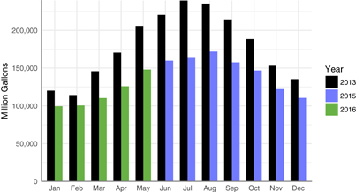
Figure 2. Reported monthly water deliveries (June 2015−May 2016) relative to 2013 baseline values.
Download figure:
Standard image High-resolution image
Figure 3. Observed water savings (a), estimated IOU electricity savings (b), and estimated total electricity savings (c) achieved over the duration of California's urban water conservation mandate.
Download figure:
Standard image High-resolution image
Figure 4. Electricity savings from IOU EE programs (July 2015–June 2016) by end-use category vs. estimated electricity savings (IOU and total) from statewide water conservation (June 2015–May 2016).
Download figure:
Standard image High-resolution imageThe savings varied significantly by hydrologic region in the state, with greatest savings occurring in the populous South Coast region (237 200 MG) and the lowest savings achieved in the sparsely populated North Lahontan region (1400 MG). Since the electricity and GHG emissions savings are calculated directly from water savings, the results of these calculations demonstrated a similar spatial variation. Figure 3 illustrates the mapped results of the estimated water (a), IOU electricity savings (b), and total electricity savings (c) for all the reporting water agencies, aggregated by the hydrologic zones.
The total estimated electricity savings associated with the observed statewide water conservation was 1830 GWh. This total quantity represents the equivalent electricity use of 274 000 average Californian homes (6680 kWh household yr−1) for a full year (EIA 2016); or, roughly 40% more electricity as produced in 2015 by the largest solar photovoltaic generation facility (the 550 MW Topaz Solar Farm) in California (CEC 2016).
Further, the total estimated electricity savings from reduced water deliveries represents about 111% of the first-year electricity savings for all the IOU EE programs (1651 GWh) funded over the reporting period from July 2015–June 2016 (figure 4). This suggests that even without specifically targeting electricity savings, the Governor's urban water conservation mandate represents 11% more statewide electricity savings than the estimated electricity savings claimed for the IOU EE programs over roughly the same time period (figure 4).

Figure 5. Comparison of LCSE achieved through statewide water conservation relative to other energy efficiency programs (adapted from Hoffman et al (2015)). 'Res' = residential; 'CI' = commercial, agricultural, and institutional; 'MUSH' = municipalities, universities, schools, and hospitals; and 'HERs' = Home Energy Reports.
Download figure:
Standard image High-resolution imageHowever, if we just look at IOU electricity savings from water conservation (605 GWh), they represent only 37% of the estimated electricity savings from the IOU EE programs. This broad differential in savings is mostly driven by the difference between total and IOU energy intensity for the South Coast region, which depends heavily on imported water from the State Water Project and the Colorado River, both of which convey water great distances using mostly non-IOU electricity sources. The South Coast also happens to be by far the largest water consumer of all the hydrologic zones in the State, so the energy intensity differential for this zone is further amplified by this higher level of consumption. In fact, the differential in the South Coast embedded electricity consumption between total and IOU electricity (1 089 600 MWh) explains roughly 89% of the statewide differential (1 225 000 MWh) in these estimates.
While figure 4 compares the quantity of electricity savings (both total and IOU) achieved through water conservation relative to the IOU EE programs over roughly the same time period, it is perhaps even more interesting to compare the cost of achieving these savings relative to the traditional EE programs. As described above, we used the LCSE indicator for this comparison, which provides a consistent metric to compare the cost per unit of electricity savings ($ MWh−1) by incorporating the persistence of the program or technology savings overtime.
Figure 5 shows the results of the LCSE comparison between the electricity savings achieved under the three scenarios of persistence for water conservation (1 year, 3.9 year, and 12 year) relative to a range of other electricity efficiency programs, with LCSE values ranging from $21 MWh−1 for residential lighting rebate programs to $149 MWh−1 for programs targeting low-income communities (Hoffman et al 2015).
As would be expected, the distinction between total and IOU electricity has a big impact on the cost-effectiveness of the estimated savings. Looking at total electricity savings, even the most conservative assumption of 1 year persistence for the water-derived electricity savings generates a competitive LCSE of $69 MWh−1. Allowing for some persistence in the savings (the 3.9 year scenario) proves to be cheaper (LCSE of $19 MWh−1) than all the electricity programs selected for comparison and the highly optimist 12 year persistence scenario would provide a rather remarkable LCSE of $7 MWh−1.
For the IOU-only savings, a 1 year persistence ($208 MWh−1) is not cost-competitive with the listed EE programs. However, assuming a reasonable 3.9 year savings persistence results in mid-scale cost-effectiveness ($57 MWh−1) and 12 year persistence ($22 MWh−1) is only marginally less competitive than the most cost-effective traditional EE program (consumer lighting product rebate).
The total estimated statewide GHG emissions savings were 521 000 MT CO2e for the period from June 2015–May 2016. This total GHG emission reduction is roughly equivalent to taking 111 000 average cars off the road for a year (EPA 2014). Using the estimated price of carbon on the California cap-and-trade market at $12.95 MT−1 CO2e (September 2016), the total value of these GHG savings is more than $6.7 M (Climate Policy Initiative 2016). The results, summarized by hydrologic region, are reported in table 1.
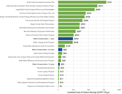
As a basis for assessing cost-effectiveness, we compared the LCSG of the water conservation mandate (using the same scenarios of persistence as for the energy savings: 1 year, 3.9 year, and 12 year) to the comparable LCSG of GHG reduction programs financed by the state's Greenhouse Gas Reduction Fund (GGRF) published by CARB (CARB 2016a) (figure 6). The GGRF is funded by the auction proceeds from the State's carbon cap-and-trade program (Assembly Bill 32 or AB 32), which amounted to roughly $1.5 billion deposited in the 2014–15 fiscal year (Rabin et al 2015). The GGRF funds are appropriated by the Governor and the State Legislature towards investments that further the core objectives of AB 32, including GHG reduction and sequestration, as well as support the broader goal of advancing a clean energy economy in California (CARB 2016b). We do not differentiate between 'total' and 'IOU' GHG savings because this distinction in the type of electricity provider is only relevant to allocation of funds for EE programs (regulated by the CPUC), and is not relevant to programs funded through the GGRF.
The GGRF-funded projects for which there are data ranged broadly from $4 MT−1 CO2e for the 'Organics and Recycling Project Loans' to $791 MT−1 CO2e for the 'Public Fleets Increased Incentives Pilot'. While not the cheapest pathway to reducing GHG emissions, the estimated LCSG for GHG reductions via urban water conservation for all three persistence scenarios ($242 MT−1 CO2e [1 year]; $66 MT−1 CO2e [3.9 year]; and, $25 MT−1 CO2e [12 year]) ranked competitively in comparison to the other GGRF-funded projects.
Figure 6. Comparing the levelized cost of saved GHGs (LCSG) savings achieved through statewide water conservation relative to GGRF program investments (CARB (2016a)).
Download figure:
Standard image High-resolution image
4. Conclusion
In the spring of 2015, more than 93% of California was experiencing 'severe drought' (The National Drought Mitigation Center 2015). In response, Governor Jerry Brown implemented the first urban water conservation mandate in the state's history. Over the period of the mandate, urban water utilities and consumers responded to the urgent need to conserve water by reducing water consumption by 24.5%. Given the linked relationship between water systems and energy use, we estimated that this large-scale effort at water conservation generated 1830 GWh of total electricity savings (605 GWh of IOU electricity savings) over the same time period. The total electricity savings, in turn, represent approximately 521 000 MT CO2e in avoided GHGs.
The scale of these integrated water-energy-GHG savings achieved over such a short period of time is remarkable, but even more interesting was the relative cost of achieving these savings through water conservation relative to existing programs that specifically target electricity or GHG reductions. While the results varied significantly based on the assumed persistence of the savings (1 year, 3.9 year, and 12 year), the majority of the scenarios explored suggested that the estimated LCSE and LCSG were well within the cost-effectiveness ranges of the existing electricity and GHG reduction programs.
These results provide strong support for including direct water conservation in the portfolio of program and technology options for reducing energy consumption and GHG emissions. This conclusion is even further strengthened considering that our analysis was based only on pursuing the individual goals of either electricity savings or greenhouse gas reductions, and not the combined benefits of water and electricity and GHG savings. Taking these three benefits into consideration together would substantially increase the cost-effectiveness of water-focused conservation programs across all scenarios of varying program and technology persistence. This finding reveals a strong incentive for water and energy utilities to form partnerships and identify opportunities to secure these combined resource savings benefits at a shared cost; and, for the associated regulatory agencies to support these partnerships through aligned policy measures and targeted funding initiatives.
While this analysis was based on the best available data, it is important to note that the water-energy-GHG savings estimates are based on relatively coarse assumptions that are also limited to the California context. Additional efforts should be pursued at a range of locations and at different scales, from the individual water utility to larger regional analyses, to produce higher resolution water-energy-GHG estimates and to capture a diversity of case examples. Further, additional research is required to go beyond the estimation of linked energy savings using static energy intensity estimates by including observable data that confirms the energy savings linked to water conservation efforts. This research can then inform more detailed models that are better able to predict and verify the timing, location, and quantity of energy savings (and GHG savings) derived from future water conservation efforts.
Footnotes
- 3
Top eight water suppliers, listed by total volume of deliveries in 2013: Los Angeles Department of Water and Power, East Bay Municipal Utilities District, City of San Diego, San Jose Water Company, City of Fresno, City of Sacramento, Coachella Valley Water District, and Eastern Municipal Water District.