

Abstract
Access to accurate, generalizable and scalable solar irradiance prediction is critical for smooth solar-grid integration, especially in the light of the accelerated global adoption of solar energy production. Both physical and statistical prediction models of solar irradiance have been proposed in the literature. Physical models require meteorological forecasts—generated by computationally expensive models—to predict solar irradiance, with limited accuracy in sub-daily predictions. Statistical models leverage in-situ measurements which require expensive equipment and do not account for meso-scale atmospheric dynamics. We address these fundamental gaps by developing a convolutional global horizontal irradiance prediction model, using convolutional neural networks and publicly accessible satellite cloud images. Our proposed model predicts solar irradiance in 12 different locations in the US for various prediction time horizons. Our model yields up to 24% improvement in an hour-ahead predictions and 26% in a day-ahead predictions compared to a persistence forecast. Moreover, using saliency maps and target-location-focused cropping, we demonstrate the benefits of incorporating meso-scale atmospheric dynamics for prediction performance. Our results are critical for energy systems planners, utility managers and electricity market participants to ensure efficient harvesting of the solar energy and reliable operation of the grid.
Export citation and abstract BibTeX RIS
1. Introduction
Harnessing solar energy is essential for paving the path toward energy sector decarbonization, a necessary step in reducing the adverse environmental and health impacts of fossil-fuel-based electricity production and decelerating climate change (Rai and Sigrin 2013). Global photovoltaic solar energy production has increased from 994 GWh in 2000, to 443 554 GWh in 2017 (IEA 2019). This rapid increase in capacity requires accurate forecasting of solar production at all levels, from rooftop to utility-scale deployment, to ensure smooth integration and reliable operation of the grid (Lorenz et al 2014, Golestaneh et al 2016). Short-term, hour- and day-ahead forecasts of renewable energy are critical for the efficient and cost effective operation of the electricity grid (Rachunok et al 2020). Specifically, short-term solar power plant predictions allow utilities and electricity market operators to make informed decisions for scheduling reserve capacity and designing efficient bidding strategies for hour-ahead and day-ahead wholesale power markets. Medium- and long-term forecasts are vital for understanding the strategic value of solar panel deployment from small-scale roof tops to grid-scale solar projects (Antonanzas et al 2016, Kaur et al 2016).
Solar energy production is predominantly a function of the characteristics of the solar panel as well as the amount of solar radiation captured (Antonanzas et al 2016). Therefore, access to accurate solar irradiance forecasts is necessary for energy systems professionals to be able to estimate solar power production at various future time horizons. Solar irradiance is typically estimated via the global horizontal irradiance (GHI), which measures the total radiation (in W m−2) from the Sun on a horizontal surface on the earth (Sengupta et al 2018). As such, GHI prediction is an integral component of forecasting solar energy output.
Previous work on predicting GHI can be classified into physical and statistical models (Antonanzas et al 2016). Physical models are based on theoretical understandings of light transmission to estimate irradiance (AghaKouchak and Nakhjiri 2012). The simplicity of theoretical transmission models makes them highly generalizeable, as irradiance is calculated based on information such as wind speed, oxygen levels, ground angle, cloud coverage, and elevation (Antonanzas et al 2016). However, these theoretical models lack the specificity required for accurate GHI forecasting (Dolara et al 2015). Another class of physical models is based on the numerical weather prediction methods that use computationally expensive simulations, which are typically run on supercomputers, with limited accuracy in sub-daily predictions (Letendre et al 2014).
Statistical models learn from historical observations and do not leverage physics-based knowledge. Instead, they are empirically driven, and predict future GHI values using statistical learning methods trained on historical data (Yang et al 2018). Statistical solar irradiance prediction methods can be sub-categorized into two paradigms: endogenous and exogenous. Endogenous models generally require ground GHI data as input, as measured by both a pyranometer and a pyrheliometer (Fuquay and Buettner 1957, Kerr et al 1967). Due to requiring the physical deployment of ground instrumentation, endogenous statistical models lack the ability to spatially generalize to locations without in-situ ground GHI measurements. Contrary to endogenous models, exogenous models utilize non-GHI data sources to predict GHI values. The current state-of-the-art in exogenous modeling uses total-sky imager—ground captured sky images (Feng and Zhang 2020). This procedure takes pictures from the ground at a specific location and utilizes a convolutional neural network to analyze captured image data to predict GHI. Other examples include recent works by Feng et al (2017), Crisosto et al (2018), Kamadinata et al (2019), Ryu et al (2019), Jiang et al (2020), Le Guen and Thome (2020), all of which involve training accurate artificial neural networks (ANNs)-based models, using ground-based cloud images, to predict GHI (the two papers are hybrid models which use endogenous GHI data as well as exogenous cloud images). However, the prediction time horizons for all these works range from 0 to a maximum of 1 h. Moreover, while classified as exogenous, this approach still requires in-situ hardware deployment to photograph the sky. Thus, it is subject to the same limitations as endogenous predictions.
Moreover, GHI is affected by both point-specific and meso-scale dynamics in atmospheric dynamics conditions (Fuquay and Buettner 1957). The majority of the current GHI prediction models do not incorporate micro- and meso-scale atmospheric dynamics at a wide scale (Antonanzas et al 2016). A notable exception is a recent model proposed by Jiang et al (2019) which incorporates meso-scale atmospheric dynamics together with point-specific locational and temporal information to estimate hourly global solar radiation in China, utilizing a deep neural network. However, their estimates are based on real-time input data and thus not suitable for hour- and day-ahead forecasting purposes. Koo et al (2020) also harnesses an exogenous approach for GHI prediction. Specifically, they train an ANN model using satellite images together with solar zenith angles and hour angles to make hourly estimations of solar energy in Korea. However, their estimation is for hourly sums instead of point estimations, and it also requires real-time data.
In this paper, we propose an exogenous approach: the convolutional global horizontal irradiance (C-GHI) model to predict GHI based on freely available cloud images obtained from geostationary satellites. This approach requires no physical instrumentation, and is easily generalizable across regions. C-GHI is based on convolutional neural networks—a non-linear deep learning technique that can learn complex information from image data. C-GHI overcomes the limitations of current statistical and physical models by accurately predicting GHI using entirely exogenous data—enabling a fully remote, worldwide GHI estimation technique, with prediction quality similar to in-situ methods. Moreover, using data-preprocessing and model inferencing techniques in a novel way, we demonstrate the benefits of leveraging a holistic approach and accounting for meso-scale dynamics in solar irradiance predictions, and illustrate model accuracy trends as a function of variable temporal prediction horizons. The structure of the paper is as follows. Section 2 summarizes the input data used in the analysis. Section 3 outlines our proposed approach. Finally, results and conclusions are presented in sections 4 and 5, respectively.
2. Data
The data utilized in this study consists of satellite images of the continental United States (CONUS) and GHI measurements from the Cooperative Network for Renewable Resource Measurements (CONFRRM). Section 2.1 describes the satellite imagery data, section 2.2 describes the solar irradiance data, and section 2.3 outlines pre-processing of the data for the analysis.
2.1. Satellite imagery
We used geostationary satellite imagery captured by NOAA's Geostationary Operational Environmental Satellite 8 (GOES8) infrared channels. The satellite imagery data is maintained by the Satellite Data Services (SDS) group at the University of Wisconsin-Madison Space Science and Engineering Center. The data was collected from Multi-format Client-agnostic File Extraction Through Contextual HTTP, a web-based API, maintained by SDS (SSEC UW-Madison 2020). Each GOES 8 image has a 2125 × 825 pixel resolution per channel. In this study, 4 infrared channels are used: channels 2–5, which operate on wavelengths: 3.9, 6.8, 10.7, and 12 µm. The spatial resolutions vary between 4 and 8 km. Figure 1 shows a sample of the input data from all 4 channels.

Figure 1. Full resolution GOES8 CONUS infrared satellite images. From (a) to (d), they are channel 2 to channel 5 imagery taken on 15 December 1999 at 19:30 GST.
Download figure:
Standard image High-resolution image2.2. Solar irradiance
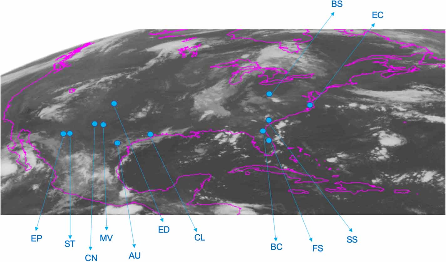
We collected solar irradiance data for 12 different stations in 7 states throughout the CONUS (figure 2): Florida (FL), Georgia (GA), Mississippi (MS), New Mexico (NM), North Carolina (NC), Texas (TX), and West Virginia (WV). Details of the 12 stations are given in table 1. The irradiance data have a 5 min temporal resolution, with the exception of Cape Canaveral FL data, with a 6 min temporal resolution. The geographic characteristics of the study sites are summarized in table 1 and figure 2, respectively. Moreover, the correlation of GHI between different case study sites are depicted in figure 3.

Figure 2. The locations of case study sites on a continental U.S. satellite imagery.
Download figure:
Standard image High-resolution image
Figure 3. Correlation of GHI values between case study sites.
Download figure:
Standard image High-resolution imageTable 1. Detailed information about the case study sites.
| Code | Name | Lat. (∘N) | Lon. (∘W) | Alt. (m) | Data size (month) |
|---|---|---|---|---|---|
| FS | Florida Solar Energy Center | 28.39 | 80.76 | 18.1 | 24 |
| BC | Bethune-Cookman College | 29.18 | 81.02 | 20.0 | 35 |
| SS | Savannah State College, GA | 32.03 | 81.07 | 11.0 | 24 |
| MV | Savannah State College, MI | 33.05 | 90.33 | 52.0 | 24 |
| ST | Southwest Technology Development Institute | 32.27 | 106.74 | 1200.9 | 15 |
| EC | Elizabeth City State University | 36.28 | 176.22 | 26.0 | 36 |
| AU | The University of Texas Austin | 30.29 | 97.74 | 21.0 | 14 |
| CN | West Texas A&M University | 34.99 | 101.90 | 1066.8 | 15 |
| ED | University of Texas Pan America | 26.20 | 98.22 | 30.0 | 13 |
| EP | University of Texas an El Paso | 31.80 | 106.40 | 1219.0 | 15 |
| CL | Lyndon B. Johnson Space Center | 29.56 | 95.12 | 33.0 | 15 |
| BS | Bluefield State College | 37.27 | 81.24 | 803.0 | 36 |
Data is available from the start of 1996 until the end of 2012. To demonstrate the applicability of our proposed approach, we train and validate our models using data from 1999 to 2001 as it is the time period with the most complete data across all the sites. However, the model can easily be extended to more recent years, which will likely result in higher predictive accuracy owing to improved resolution of satellite imagery over time.
2.3. Data processing
Both GOES8 images and GHI data are preprocessed to facilitate statistical modeling. GOES8 images are downscaled into 256 × 256 resolution using bicubic interpolation to reduce computation time. All 4 image channels are then converted into one 256 × 256 × 4 tensor (i.e. matrix)—each entry in the tensor corresponds to one pixel in each of the 4 channels. Input data are also normalized to values in [0,1]. Missing data—caused by technical failure, regular maintenance of GOES8 systems, or missing/cracked imagery—are removed. In preprocessing of GHI data, night-time values—GHI values less than 10 W m−2—are removed. Similarly, unreliable irradiance measurements are removed based on quality control flags 4 provided by NREL's CONFRRM data (SERI 1988).
3. Methods
The proposed C-GHI prediction model is grounded in convolutional neural networks. In this section, we provide a brief overview of the model formulation (section 3.1), the technical details needed to replicate our experiment (section 3.2), model inferences (section 3.3), and measures of model performance (section 3.4).
3.1. Convolutional neural networks
ANNs are a statistical learning technique inspired by the way neurons work in the human brain. They consist of a series of neurons (i.e. nodes) which activate each other in parallel or in sequence. Each neuron and its connections are called a perceptron. Mathematically, this consists of a combination of multivariate linear regressions followed by a non-linear transformation. The non-linear transformation—called an activation function—is typically applied on the output of a perceptron.
A 'vanilla' version of a neural network algorithm consists of multiple layers of perceptrons. A neural network can learn the complex non-linear mapping between input and target variables by stacking multiple non-linear functions. A mathematical representation of a layer of a fully connected network can be written as:

where fi (X) is the output of ith layer given input X; Wi and bi are the weight tensor and bias of ith layer respectively; and a(·) is a non-linear activation function.
The output of the last layer (fN (X)) is the prediction value given an input X, where N is the number of hidden layers of a model. A neural network with more than 2 hidden layers is considered a 'deep' network. The training of a neural network is done by finding the weights which minimize the distance between the prediction values and the ground-measured observations (distance is represented by a loss function).
Convolutional neural networks (CNNs) are a class of deep neural network commonly used for image analysis (Bishop 2006). CNNs take in an input image, assign importance to visual features in the image, and ultimately make predictions about the image's contents. They are typically used for image classification, object detection and segmentation (LeCun et al 2015), and have been used in several environmental applications including urban expansion detection (He et al 2019), biophysical modeling of crop growth (Lin et al 2020), and environmental and water management (Sun and Scanlon 2019).
CNNs differ from ANNs in the way in which the layers connect. Contrary to ANN, in a CNN, a neuron of a convolutional layer takes only a portion of the output of the previous layer as its input; this portion is called a receptive field. Within a layer, each neuron has a similar sized receptive field generated with the same weights and biases, called a kernel. Convolutional layers generally utilize a linear kernel followed by a non-linear activation. To generate the output of the layer, it slides the kernel throughout the input. This sliding is called a convolution operation. A formula of a 2D convolutional layer can be written as:

where (x, y) is one entry in the output tensor of (i + 1)th layer, h is a two-dimensional kernel consisting of  weights (which are shared in the layer for every (x, y)), fi
is the output of ith layer, and a(·) is an activation function.
weights (which are shared in the layer for every (x, y)), fi
is the output of ith layer, and a(·) is an activation function.
As a way to maintain data dimensions, padding (usually zero padding) and stride values can be adjusted. Padding refers to adding extra (non-informative) pixels around the input images to keep size of output after a convolution, and stride refers to a step size that a kernel slides. A pooling layer, which performs a similar operation to a convolution but applies predefined summary function instead of convolution kernel, may also be applied after a convolutional layer to reduce dimension and reduce over-fitting. Two most common pooling methods are max-pooling and average-pooling. Max-pooling takes a maximum function for the summary function and average-pooling takes average function. As a result of this convolution operation, the (x, y)'s value of the output tensor can hold the information of multiple neighboring pixels in the input image (i.e. receptive field). By stacking multiple convolutional layers, each neurons of the output of the last convolutional layer encompasses a very large receptive field with respect to the input image.
3.2. Model specification
The CNN model structure used in our proposed C-GHI model is based on the VGG16 model (Simonyan and Zisserman 2014), with adjustments made for the number of layers and regularization parameters for each study site. We build separate models for each region and time horizon, using the same network architecture briefly described below. The convolutional layers receive the input image in series, each of which with filter size 32, 64, 64, 128, 128, and, 128. The convolutional kernel size is 3, and the stride is 1, in all layers. Max-pooling is applied after every other layer with kernel size 3, 3, and 2 respectively. After the convolutional layers, the data is passed through three fully connected layers—with 1024, 1024, and 1 nodes respectively. Rectified linear unit, a type of non-linear activation function, is also applied for every layer except for the last fully connected layer. Additional L2-regularization with respect to all weights is added to the loss function to reduce the risk of over-fitting. In short, the final loss function is  , where MSE stands for mean squared error. Lastly, Adam Optimizer is utilized (Kingma and Ba 2015) to tune the model weights, given the input dataset.
3.3. Feature visualization
As a posterior analysis, we apply feature visualization techniques to the fitted models to visualize model performance at different spatial and temporal scales. Specifically, we harness saliency maps for the model inference. Saliency maps help visualize the gradient of the cost function with respect to each pixel of the input (Simonyan et al
2013). In other words, saliency maps involve calculating ![$[\partial E^j/\partial X]_{X = X^j}$](https://content.cld.iop.org/journals/1748-9326/16/4/044045/revision3/erlabe06dieqn3.gif) , where Ej
is the prediction error of jth observation, X is the variable indicating an image, and Xj
is the jth image. The gradient is then projected onto the original image plane. Saliency maps (figure 4) show the effect of a unit change in a pixel on the prediction accuracy. If the gradient of a pixel is higher, it indicates that the pixel is more informative for the particular prediction.
, where Ej
is the prediction error of jth observation, X is the variable indicating an image, and Xj
is the jth image. The gradient is then projected onto the original image plane. Saliency maps (figure 4) show the effect of a unit change in a pixel on the prediction accuracy. If the gradient of a pixel is higher, it indicates that the pixel is more informative for the particular prediction.

Figure 4. Saliency maps. From top to bottom, they are for 5 min, 1 h, 1 d ahead predictions. The four regions represent regions with the least correlation between each other. From (a) to (d), they are of region AU, BC, CL and ST respectively. In these images, lighter regions have a higher gradient, thus lighter regions have a higher contribution to the GHI prediction. The red triangles on the images represent the location of each region.
Download figure:
Standard image High-resolution image3.4. Model performance
In our experiments, two model performance metrics are used: mean-squared error (MSE), and root mean-squared error (RMSE). For parameter tuning in fitting each model, we use MSE, mathematically represented as:

where yi
and  are the ground-measured and predicted GHI of ith observation respectively.
RMSE is used in comparing the predictive performance of different models. We report RMSE as it is a widely applied metric for solar irradiance prediction, particularly in exogenous predictive models. Additional performance metrics of MAPE, R2, and nRMSE are also calculated and included in the appendix tables A3–A5.
Since two different GHI prediction models cannot be directly compared if the prediction regions, time, and temporal horizons do not match, and there is no agreed upon benchmark dataset, we compare our models' performance against the persistence model which is represented as:

where  is the predicted GHI at time t and y(t) is the observed GHI at time t, and T is the prediction interval. In essence, the persistence model assumes all future predictions will be equal to the last observed value at T time before.
4. Results and discussion
Comparing model performance of both the persistence and C-GHI prediction indicates that the C-GHI outperforms the persistence model in all but one location for day-ahead predictions, and in all hour-ahead predictions. The persistence model demonstrates better performance in 30 min predictions across all regions, which is not surprising given the temporal auto-correlation in GHI values. We hypothesize that the poor performance of the CNN-based model in the EP region 1 d ahead forecasting compared to the persistence is due to a 24 h lagged auto-correlation within the GHI data measured at the site. Results in units of RMSE are presented for all temporal horizons for four regions with minimal correlation in table 2, and a comparison between the C-GHI and persistence models are shown in table 3. Results for all locations are shown in appendix tables A6 and A7.
Table 2. Performance RMSE (W m−2) by prediction horizon and region. AU (the University of Texas Austin), BC (Bethune-Cookman College), CL (Lyndon B. Johnson Space Center), ST (Southwest Technology Development Institute). Prediction lead-times with the lowest RMSE for each location are bolded.
| AU | BC | CL | ST | |||||
|---|---|---|---|---|---|---|---|---|
| Time (min) | Train | Test | Train | Test | Train | Test | Train | Test |
| 5 | 83.49 | 190.06 | 134.62 | 166.01 | 154.35 | 191.59 | 79.40 | 141.60 |
| 10 | 112.35 | 195.58 | 118.85 | 171.34 | 160.21 | 186.42 | 80.25 | 143.36 |
| 15 | 137.03 | 195.42 | 142.79 | 168.19 | 161.95 | 188.15 | 99.44 | 145.26 |
| 20 | 125.94 | 197.90 | 144.14 | 166.90 | 148.96 | 193.36 | 104.17 | 147.22 |
| 25 | 125.42 | 198.64 | 139.31 | 169.80 | 148.96 | 193.36 | 118.91 | 153.43 |
| 30 | 134.35 | 199.23 | 147.61 | 172.49 | 163.16 | 195.01 | 122.82 | 157.45 |
| 60 | 101.74 | 191.71 | 148.56 | 177.26 | 162.80 | 189.48 | 93.96 | 158.20 |
| 1440 | 139.23 | 200.54 | 159.27 | 191.11 | 182.45 | 207.87 | 137.42 | 161.44 |
Table 3. Comparison in RMSE (W m−2) with persistence model as a benchmark.
| AU | BC | CL | ST | |||||
|---|---|---|---|---|---|---|---|---|
| Time (min) | Perst | C-GHI | Perst | C-GHI | Perst | C-GHI | Perst | C-GHI |
| 30 | 147.55 | 199.23 | 160.65 | 172.49 | 164.28 | 195.01 | 126.83 | 157.45 |
| 60 | 199.97 | 191.71 | 215.84 | 177.26 | 213.98 | 189.48 | 198.44 | 158.20 |
| 1440 | 241.31 | 200.54 | 224.66 | 191.11 | 252.02 | 207.87 | 179.89 | 161.44 |
These results indicate that the RMSE of both the C-GHI and persistence model generally increase as the time horizon increases. However, the C-GHI model's performance remains largely consistent in farther-ahead predictions across all regions. In contrast, the persistence model's performance decreases significantly as the time horizon increases. In the BS region, for example, the persistence model's day-ahead RMSE is 64% greater than the 30 min prediction. By contrast, the C-GHI model's RMSE increases only by 0.6%.
The C-GHI outperforms the persistence model by an average of 14.39% in hour-ahead prediction, and 13.35% in day-ahead prediction across all locations. This indicates that, within a single region, the prediction error increases slowly as the temporal prediction horizon increases when utilizing a satellite image based model. We also see comparable results between the C-GHI and other state-of-the-art exogenous models. Direct comparisons between GHI prediction models is not possible because of differences in prediction regions, temporal horizons, and available data. Accordingly, we utilize percentage improvement over a persistence model to compare modeling techniques with different temporal and spatial characteristics. Using this metric, C-GHI model's performance is on par with current state-of-the-art exogenous models' performance in terms of percentage improvements from the persistence model.
We compare the C-GHI to two other comparable exogenous GHI prediction models. The first model, proposed by Feng and Zhang (2020), utilizes a total-sky image (thus not fully exogenous) and is trained on 3 years of data at NREL's South table Mountain Campus, Golden, Colorado. The 1 h ahead prediction performance compared to persistence is 34.02%. The best C-GHI performance for 1 h ahead prediction is 24.26% at CN region. Qing and Niu (2018) proposed a 1 d ahead time-series model to predict GHI using weather forecast datasets. Their model for Santiago in Cape Verde utilizes 30 months of data, which is a similar data size to our dataset, and showed 30.68% performance improvement over the persistence model. This is comparable to our best 1 d ahead model in BS region, which showed 25.52% improvement.
4.1. Model visualization
We hypothesize that the model prediction quality is the result of the C-GHI locating the prediction region and adjusting the size and scope of the input data. That is, given the whole US satellite imagery and historical GHI data for a specific point, the learning process encourages the C-GHI to seek out the prediction location and a sufficient surrounding area to optimally map an input to an output.
To test this hypothesis, we leverage saliency maps (introduced in section 3.3) to understand the geographic regions which most contribute to the GHI prediction. An example is illustrated in figure 4. In these maps, lighter colors indicate regions of higher gradients with respect to the prediction and thus a greater contribution to GHI prediction. In each location, the brighter region becomes wider and more diffuse around the correct region as the prediction horizon grows.
4.2. Deterministic cropping
The C-GHI demonstrates high predictive accuracy when the entire CONUS imagery is utilized to predict local GHI values. In order to understand which areas of the country contribute to a particular regional GHI prediction, we perform the same analysis, but crop the input images to a specific window around the prediction location. We apply fixed-location deterministic cropping as a data pre-processing step, given the target prediction region's location. By fitting and comparing models for different cropping sizes and prediction horizons, we aim to understand the extent to which increased regional information improves prediction accuracy across different prediction horizons.
What follows is an example of the cropping procedure at the AU location for one channel. First, we calculate the location of the AU site (lat, lon) = (30.29∘ N, 97.74∘ W) within the satellite imagery. Each image is then centered around the AU site and cropped into squares with side lengths of: 10, 20, 40, 60, 100, 140, 180, 220, 260, 300, 360, 420, and 512 pixels. All cropped images are resized to 256 × 256 using bicubic interpolation to preserve the network architecture and maintain the number of parameters within the C-GHI. Finally, each model is separately trained per cropping window size and time horizon using the same dataset. We show the results of the predictions in figure 5.

Figure 5. Model performance as a function of cropping window and temporal scale across multiple locations. Initial increases in cropping window significantly improve model performance, however, the improvements diminish as the window expands. The x-axes in the figure represent the side length of the original cropping window, and the y-axes represent RMSE. Dotted lines represent the performance of a model with no cropping. (data in table A1)
Download figure:
Standard image High-resolution imageResults indicate that prediction error decreases rapidly in 5 min and 1 h prediction as a result of increasing cropping window size when window size is small, and prediction error levels off as the window size becomes very large. Additionally, the effect of increasing the cropping window size become weaker in longer-term prediction. In figure 5, for 5 min ahead prediction in AU, the cropped-image model surpasses the error of full-size-image model at approximately 30 000 pixels—the result of a cropping window of 180 × 180. For 1 h ahead prediction, this threshold increases to 150 000 pixels (roughly 380 × 380). For 1 d ahead prediction, the threshold is approximately 230 000 pixels (480 × 480). As all cropped-image models surpass the predictive quality of full-size-image models, we conclude that regional image cropping is beneficial to GHI prediction, particularly in short-term prediction.
Additionally, we find that the predictive performance of models with noisy saliency maps (i.e. 5 min ahead prediction in AU and CL) is substantially improved when input images are cropped. We believe this is due to the model identifying the prediction location more accurately in longer temporal horizons and the the wider regional cloud information surrounding the target point which can be incorporated. For example, the 5 min ahead prediction in AU had an 8.2% improvement by the method at window size 300 × 300, while the 5 min ahead prediction in BC had only a 4.0% improvement even at 512 × 512. We can see that in figure 4 the saliency map of AU in the 5 min ahead prediction is noisier than that of BC. The ability of the CNN-based model to maintain predictive accuracy at increased time horizons combined with the benefits to model accuracy gained by cropping the input image reveals that the C-GHI is accurately capturing the regional meteorological patterns which contribute to GHI values. The cropping window size required to achieve similar performance to an uncropped model increases as the prediction horizon increases.
4.3. Weather condition effects
Lastly, we test the sensitivity of C-CHI's prediction performance to the degree of cloud cover, focusing on the best performing regions of ED and BC. ED, located in McAllan, Texas, has a semi-arid climate under the Köppen climate classification; it has very hot and humid summers and short and warm winters. BC, located in Daytona Beach, Florida, has a humid subtropical climate with warm and wet summers and cooler and drier winters. These two regions have similar climatological characteristics, but ED is drier and hotter.
To assess the sensitivity of model performance to degree of cloud cover, we first label the days in the model as 'sunny', 'partly cloudy', and 'cloudy'. The labels are chosen based on data from the Weather Underground (The Weather Underground 2020). We looked at daily rather than hourly weather data, following the convention in the solar irradiance prediction literature. The cloud cover labels are selected based on the following criteria: (i) 'sunny' represents days with more than 90% clear sky conditions, or with more than 80% clear skies, with the remaining being partly cloudy; (ii) 'cloudy' represents days with either no clear sky conditions, or when more than 70% of the day is mostly cloudy and/or cloudy; and (iii) 'partly cloudy' represent days that are neither completely sunny nor cloudy.
Table 4 shows the test set performance changes over different cloud cover conditions and prediction time horizons. Results indicate that as the prediction time horizon increases, C-GHI performs better than the persistence model, especially in cloudy and partly cloudy days. We find that persistence model performs well in day-ahead predictions during sunny days, possibly due to high auto-correlation in consecutive sunny days. We also find that predictions with longer lead times tend to overestimate irradiance in cloudy days and underestimate irradiance in sunny days to minimize the total sum of squared error (figure 6). We hypothesize that this helps C-CHI to better fit partly cloudy days which are most frequent in both regions, thus the overall performance benefits.

Figure 6. Scatterplots of ground-measured and predicted GHI. The images in row (a) are for the ED region and the images in row (b) are for the BC region; from left to right, the images represent models' fits for sunny, partly cloudy, and cloudy days.
Download figure:
Standard image High-resolution image
Table 4. Performance changes of (a) ED and (b) BC regions depending on weather conditions. The percentage values in parentheses under each weather condition are the proportion of the type of weather.
| 30 min | 1 h | 1 d | |||||||
|---|---|---|---|---|---|---|---|---|---|
| Weather | Improvement | Improvement | Improvement | ||||||
| condition | Perst. | C-GHI | (%) | Perst. | C-GHI | (%) | Perst. | C-GHI | (%) |
| Sunny (43%) | 83.10 | 129.02 | −55.26 | 167.18 | 140.54 | 15.93 | 140.71 | 180.62 | −28.36 |
| Partly cloudy (45%) | 120.46 | 184.15 | −52.87 | 216.09 | 172.63 | 20.11 | 222.31 | 158.45 | 28.73 |
| Cloudy (12%) | 71.67 | 187.07 | −161.03 | 144.45 | 228.20 | −53.98 | 195.74 | 138.25 | 29.37 |
| (a) | |||||||||
| 30 min | 1 h | 1 d | |||||||
| Weather | Improvement | Improvement | Improvement | ||||||
| condition | Perst. | C-GHI | (%) | Perst. | C-GHI | (%) | Perst. | C-GHI | (%) |
| Sunny (33%) | 108.65 | 131.63 | −21.15 | 171.27 | 128.90 | 24.74 | 138.02 | 137.38 | 0.46 |
| Partly cloudy (50%) | 167.25 | 168.01 | −0.45 | 222.50 | 166.13 | 25.33 | 218.34 | 176.62 | 19.10 |
| Cloudy (17%) | 147.17 | 149.27 | −1.42 | 197.19 | 161.90 | 17.90 | 240.02 | 177.54 | 26.03 |
| (b) | |||||||||
Assessing the C-CHI's prediction performance as a function of cloud types is not within the scope of this paper. However, it should be highlighted that future work analyzing the effect of cloud types on CNN-based solar irradiates prediction performance will be of great value to renewable energy planners, operators and regulators.
5. Conclusion
We propose a novel solar irradiance prediction model, using convolutional neural networks and cloud imagery. The proposed C-GHI is entirely exogenous, predicting solar irradiance based on freely-available satellite imagery of clouds. The model's performance is tested throughout various prediction horizons and compared with the persistence model across different regions. The experiment results show that the C-GHI model is highly generalizable and is robust against changes in prediction horizon and locations. The persistence model outperforms C-GHI for sub-hourly predictions, owing to the temporal auto-correlation in the GHI data. However, C-GHI's predictive performance remains steady with increasing lead times, while the performance of the persistence model decreases significantly as the prediction horizons increase. C-GHI outperforms the persistence model by up to 26% in day-ahead prediction.
Using saliency maps as a inferencing tool, we find that model's improved accuracy can be attributed to the holistic approach of the CNN which includes region specific information and surrounding regions' information which are particularly helpful for long-term prediction. Additionally, we test image cropping as a method for data preprocessing and find it improves model performance in all prediction horizons, and is extremely beneficial in short-term GHI prediction. When an appropriate window size is selected, the cropped model outperforms the model with full CONUS imagery.
While our proposed holistic approach yields high accuracy, there are additional avenues for model improvements, for example by incorporating information such as wind speed and direction. Including such environmental factors could lead to higher prediction accuracy while still providing a fully-exogenous GHI prediction framework. Future approaches could add such temporal information through the use of time-series methods such as recurrent neural networks (LeCun et al 2015). Moreover, future extensions of this work that accounts for the influence of cloud types, collected through ceilometers, on the performance of irradiance prediction models will of great interest to renewable energy policymakers and practitioners.
In summary, the improved accuracy in predicting GHI provided by the C-GHI combines the benefits of physical GHI prediction models—namely, no need for in-situ measurement—with the accuracy of statistical models. This flexibility can allow for a low-cost exploration of PV siting locations at both a household and utility scale. More accurate GHI forecasts can also help utility-scale integration of renewable energy into the electricity grid. The uncertainty in day-ahead renewable energy production is a major hurdle to the cost-effective usage of renewable energy, and improving the accuracy of solar energy production forecasts will be vital to effectively utilizing renewable resources.
Acknowledgments
The authors would like to acknowledge Purdue Climate Change Research Center (PCCRC), the Center for Environment (C4E) as well as the NSF Grants CRISP-1832688 and CMMI-1826161.
Data availability statement
The data that support the findings of this study are openly available at the following URL/DOI: www.nrel.gov/grid/solar-resource/confrrm.html.
Appendix.: Supplementary tables
Table A1. Cropped Models RMSE (W m−2) by prediction horizon and side length of the crop window. From (a) to (d), they are of region BC, AU, CL and ST respectively.
| Side length | |||||||||||||
|---|---|---|---|---|---|---|---|---|---|---|---|---|---|
| Time (min) | 10 | 20 | 40 | 60 | 100 | 140 | 180 | 220 | 260 | 300 | 360 | 410 | 512 |
| 5 | 245.55 | 238.95 | 229.51 | 218.62 | 210.11 | 204.82 | 190.06 | 181.72 | 178.25 | 174.44 | 179.75 | 182.28 | 185.66 |
| 60 | 239.94 | 235.71 | 223.92 | 219.78 | 216.65 | 213.44 | 214.41 | 206.36 | 197.68 | 195.06 | 192.82 | 189.22 | 187.33 |
| 1440 | 259.53 | 254.85 | 250.46 | 248.52 | 235.19 | 229.93 | 220.79 | 215.55 | 205.42 | 204.68 | 201.31 | 201.70 | 199.71 |
| (a) | |||||||||||||
| Side length | |||||||||||||
| Time (min) | 10 | 20 | 40 | 60 | 100 | 140 | 180 | 220 | 260 | 300 | 360 | 410 | 512 |
| 5 | 232.43 | 223.02 | 207.90 | 189.01 | 171.68 | 167.82 | 167.24 | 167.43 | 166.13 | 165.26 | 163.63 | 159.51 | 159.42 |
| 60 | 259.63 | 253.37 | 238.60 | 228.30 | 222.53 | 213.18 | 207.65 | 202.83 | 200.38 | 190.79 | 187.23 | 176.16 | 172.77 |
| 1440 | 251.73 | 244.99 | 238.04 | 230.89 | 223.92 | 217.01 | 209.25 | 207.71 | 206.07 | 204.59 | 200.08 | 194.77 | 190.48 |
| (b) | |||||||||||||
| Side length | |||||||||||||
| Time (min) | 10 | 20 | 40 | 60 | 100 | 140 | 180 | 220 | 260 | 300 | 360 | 410 | 512 |
| 5 | 228.45 | 223.90 | 217.25 | 209.68 | 205.55 | 199.71 | 196.72 | 194.41 | 185.22 | 181.06 | 181.89 | 184.54 | 179.54 |
| 60 | 241.55 | 239.24 | 235.36 | 226.25 | 211.18 | 210.30 | 208.09 | 205.88 | 202.30 | 200.24 | 198.84 | 196.36 | 192.46 |
| 1440 | 232.59 | 226.67 | 224.36 | 221.99 | 219.58 | 219.60 | 213.39 | 214.96 | 212.75 | 210.28 | 209.64 | 206.39 | 202.98 |
| (c) | |||||||||||||
| Side length | |||||||||||||
| Time (min) | 10 | 20 | 40 | 60 | 100 | 140 | 180 | 220 | 260 | 300 | 360 | 410 | 512 |
| 5 | 182.73 | 175.24 | 166.24 | 165.10 | 155.82 | 153.44 | 150.16 | 148.23 | 145.79 | 144.57 | 143.73 | 143.30 | 140.66 |
| 60 | 219.14 | 210.11 | 199.20 | 185.74 | 179.89 | 178.98 | 176.13 | 170.10 | 167.77 | 167.50 | 163.53 | 162.03 | 157.62 |
| 1440 | 196.52 | 187.63 | 184.25 | 184.39 | 173.17 | 169.98 | 164.59 | 163.29 | 160.51 | 158.98 | 159.78 | 158.03 | 155.35 |
| (d) | |||||||||||||
Table A2. C-GHI: best performance regions per time horizon are presented (no cropping); (a): Ryu et al (2019) used CNN with Total-sky Imager data; (b): Qing and Niu (2018) used LSTM (time-series) with weather forecast data.
| Model | Time (min) | Data size (month) | Persistence RMSE | Model RMSE | Improvement (%) |
|---|---|---|---|---|---|
| C-GHI (BC) | 30 | 35 | 160.65 | 172.49 | −7.37 |
| C-GHI (CN) | 60 | 15 | 109.67 | 83.06 | 24.26 |
| C-GHI (BS) | 1440 | 36 | 287.95 | 214.44 | 25.52 |
| (a) (sunny) | 20 | 1/3 | 58 | 186 | −220.68 |
| (a) (cloudy) | 20 | 1/3 | 121 | 150 | −23.96 |
| (a) (overcast) | 20 | 1/3 | 91 | 111 | −21.97 |
| (b) | 1440 | 30 | 177.031 | 122.7174 | 30.68 |
| (b) | 1440 | 132 | 209.2509 | 76.245 | 63.56 |
Table A3. MAPE by prediction horizon and region. FS (Florida Solar Energy Center), BC (Bethune-Cookman College), SS (Savannah State College in Georgia), MV (Savannah State College in Michigan), ST (Southwest Technology Development Institute), EC (Elizabeth City State University), AU (the University of Texas Austin), CN (West Texas A&M University), ED (University of Texas Pan America), EP (University of Texas an El Paso), CL (Lyndon B. Johnson Space Center), and BS (Bluefield State College).
| FS | BC | SS | MV | ST | EC | AU | CN | ED | EP | CL | BS | |||||||||||||
|---|---|---|---|---|---|---|---|---|---|---|---|---|---|---|---|---|---|---|---|---|---|---|---|---|
| Time (min) | Train | Test | Train | Test | Train | Test | Train | Test | Train | Test | Train | Test | Train | Test | Train | Test | Train | Test | Train | Test | Train | Test | Train | Test |
| 5 | 28.02 | 32.62 | 22.69 | 29.24 | 19.66 | 30.72 | 24.55 | 30.72 | 11.67 | 21.98 | 29.26 | 35.75 | 14.73 | 36.44 | 35.93 | 41.22 | 21.90 | 33.81 | 15.45 | 31.99 | 28.56 | 36.18 | 25.23 | 39.23 |
| 10 | 29.36 | 33.54 | 19.42 | 29.09 | 21.42 | 30.84 | 21.82 | 30.38 | 11.64 | 22.15 | 29.18 | 35.97 | 20.16 | 37.64 | 38.75 | 42.25 | 28.75 | 34.98 | 16.22 | 32.09 | 30.41 | 36.18 | 32.25 | 41.46 |
| 15 | 29.74 | 33.93 | 24.62 | 29.66 | 21.00 | 30.21 | 22.19 | 31.62 | 14.98 | 22.74 | 24.73 | 35.67 | 26.08 | 38.41 | 37.21 | 41.96 | 25.70 | 33.87 | 23.67 | 32.79 | 30.53 | 36.08 | 29.03 | 39.31 |
| 20 | 29.98 | 32.76 | 24.36 | 29.66 | 22.69 | 31.39 | 22.64 | 31.16 | 15.85 | 22.92 | 27.45 | 35.14 | 23.14 | 38.87 | 38.97 | 44.58 | 25.26 | 34.26 | 21.32 | 31.75 | 27.13 | 36.40 | 33.29 | 38.67 |
| 25 | 31.84 | 34.46 | 23.32 | 29.45 | 21.32 | 29.91 | 25.36 | 31.51 | 18.65 | 24.12 | 26.14 | 36.62 | 23.42 | 39.11 | 38.16 | 44.04 | 27.13 | 35.24 | 25.04 | 33.28 | 30.70 | 36.23 | 32.90 | 40.38 |
| 30 | N/A | N/A | 25.10 | 29.95 | 26.00 | 31.42 | 22.79 | 31.59 | 20.19 | 25.04 | 30.11 | 38.11 | 25.54 | 39.10 | 40.56 | 44.70 | 25.84 | 35.01 | 22.75 | 34.56 | 30.73 | 37.69 | 30.96 | 40.11 |
| 60 | 28.67 | 33.62 | 25.02 | 30.16 | 21.01 | 32.46 | 21.10 | 30.23 | 14.06 | 22.39 | 18.50 | 38.95 | 18.62 | 37.04 | 31.50 | 40.40 | 28.11 | 34.52 | 11.65 | 30.72 | 30.94 | 36.81 | 32.71 | 42.80 |
| 1440 | 27.37 | 35.63 | 28.40 | 34.33 | 29.37 | 34.81 | 32.92 | 35.87 | 21.45 | 24.88 | 37.63 | 45.68 | 26.73 | 38.50 | 41.99 | 60.52 | 31.07 | 35.24 | 25.80 | 33.70 | 35.78 | 39.80 | 41.45 | 47.75 |
Table A4. R-square by prediction horizon and region.
| FS | BC | SS | MV | ST | EC | AU | CN | ED | EP | CL | BS | |||||||||||||
|---|---|---|---|---|---|---|---|---|---|---|---|---|---|---|---|---|---|---|---|---|---|---|---|---|
| Time (min) | Train | Test | Train | Test | Train | Test | Train | Test | Train | Test | Train | Test | Train | Test | Train | Test | Train | Test | Train | Test | Train | Test | Train | Test |
| 5 | 0.7320 | 0.6322 | 0.8038 | 0.7070 | 0.8507 | 0.6609 | 0.7955 | 0.6676 | 0.9246 | 0.7594 | 0.7597 | 0.6528 | 0.9156 | 0.5652 | 0.6540 | 0.5261 | 0.8216 | 0.6020 | 0.9089 | 0.6109 | 0.6905 | 0.5010 | 0.8280 | 0.6188 |
| 10 | 0.7193 | 0.6280 | 0.8471 | 0.6879 | 0.8217 | 0.6554 | 0.8274 | 0.6763 | 0.9230 | 0.7535 | 0.7547 | 0.6425 | 0.8434 | 0.5315 | 0.5857 | 0.4944 | 0.8224 | 0.6020 | 0.8849 | 0.6033 | 0.6666 | 0.5275 | 0.7436 | 0.5981 |
| 15 | 0.7161 | 0.6339 | 0.7793 | 0.6993 | 0.8228 | 0.6536 | 0.8262 | 0.6650 | 0.8817 | 0.7469 | 0.8110 | 0.6516 | 0.7671 | 0.5321 | 0.6240 | 0.5231 | 0.7618 | 0.6124 | 0.7944 | 0.5976 | 0.6594 | 0.5192 | 0.7763 | 0.6091 |
| 20 | 0.6950 | 0.6326 | 0.7751 | 0.7039 | 0.8049 | 0.6407 | 0.8199 | 0.6605 | 0.8702 | 0.7400 | 0.7785 | 0.6606 | 0.8033 | 0.5200 | 0.5992 | 0.4490 | 0.7707 | 0.6168 | 0.8198 | 0.6035 | 0.7118 | 0.4923 | 0.7183 | 0.6304 |
| 25 | 0.6787 | 0.6128 | 0.7900 | 0.6935 | 0.8165 | 0.6587 | 0.7832 | 0.6609 | 0.8309 | 0.7175 | 0.7927 | 0.6342 | 0.8049 | 0.5164 | 0.6030 | 0.4823 | 0.7379 | 0.5956 | 0.7794 | 0.5897 | 0.6543 | 0.5121 | 0.7256 | 0.6072 |
| 30 | N/A | N/A | 0.7641 | 0.6837 | 0.7605 | 0.6463 | 0.8176 | 0.6505 | 0.8196 | 0.7025 | 0.7532 | 0.6239 | 0.7762 | 0.5135 | 0.5806 | 0.4788 | 0.7611 | 0.5986 | 0.8040 | 0.5716 | 0.6577 | 0.4834 | 0.7502 | 0.6070 |
| 60 | 0.7262 | 0.6405 | 0.7625 | 0.6749 | 0.8427 | 0.6330 | 0.8498 | 0.6953 | 0.8930 | 0.7050 | 0.9027 | 0.6084 | 0.8716 | 0.5497 | 0.7465 | 0.5231 | 0.7328 | 0.6178 | 0.9431 | 0.5935 | 0.6630 | 0.5216 | 0.7425 | 0.5803 |
| 1440 | 0.7502 | 0.5846 | 0.7267 | 0.6025 | 0.6993 | 0.5655 | 0.6604 | 0.5981 | 0.7749 | 0.6863 | 0.6222 | 0.4046 | 0.7629 | 0.4937 | 0.5050 | 0.2777 | 0.6846 | 0.6127 | 0.7636 | 0.5762 | 0.5641 | 0.4341 | 0.6012 | 0.5020 |
Table A5. nRMSE by prediction horizon and region; range is used for dividends.
| FS | BC | SS | MV | ST | EC | AU | CN | ED | EP | CL | BS | |||||||||||||
|---|---|---|---|---|---|---|---|---|---|---|---|---|---|---|---|---|---|---|---|---|---|---|---|---|
| Time (min) | Train | Test | Train | Test | Train | Test | Train | Test | Train | Test | Train | Test | Train | Test | Train | Test | Train | Test | Train | Test | Train | Test | Train | Test |
| 5 | 14.00 | 16.06 | 11.37 | 14.04 | 8.53 | 12.74 | 11.20 | 13.95 | 6.49 | 11.58 | 10.43 | 12.66 | 6.98 | 15.89 | 8.76 | 10.10 | 11.48 | 17.00 | 7.15 | 14.54 | 13.31 | 16.53 | 9.67 | 14.49 |
| 10 | 14.33 | 16.16 | 10.05 | 14.49 | 9.33 | 12.85 | 10.29 | 13.77 | 6.56 | 11.73 | 10.53 | 12.83 | 9.39 | 16.35 | 9.59 | 10.43 | 14.33 | 17.13 | 8.04 | 14.69 | 13.82 | 16.08 | 11.80 | 14.89 |
| 15 | 14.41 | 16.03 | 12.08 | 14.23 | 9.30 | 12.88 | 10.33 | 14.01 | 8.13 | 11.88 | 9.25 | 12.67 | 11.45 | 16.33 | 9.13 | 10.13 | 13.27 | 16.80 | 10.75 | 14.80 | 13.97 | 16.23 | 11.02 | 14.68 |
| 20 | 14.93 | 16.05 | 12.19 | 14.12 | 9.75 | 13.12 | 10.51 | 14.10 | 8.52 | 12.04 | 10.01 | 12.50 | 10.53 | 16.54 | 9.43 | 10.89 | 13.02 | 16.71 | 10.06 | 14.69 | 12.85 | 16.68 | 12.37 | 14.27 |
| 25 | 15.33 | 16.48 | 11.78 | 14.36 | 9.46 | 12.79 | 11.53 | 14.10 | 9.73 | 12.55 | 9.68 | 12.98 | 10.48 | 16.60 | 9.39 | 10.54 | 13.92 | 17.17 | 11.14 | 14.97 | 14.07 | 16.35 | 12.21 | 14.71 |
| 30 | N/A | N/A | 12.49 | 14.59 | 10.81 | 13.02 | 10.58 | 14.30 | 10.05 | 12.88 | 10.57 | 13.17 | 11.23 | 16.65 | 9.65 | 10.60 | 13.29 | 17.11 | 10.49 | 15.26 | 14.00 | 16.82 | 11.65 | 14.71 |
| 60 | 14.10 | 16.19 | 12.58 | 15.01 | 8.90 | 13.48 | 9.77 | 13.58 | 7.94 | 12.95 | 6.67 | 13.49 | 8.50 | 16.02 | 7.33 | 9.48 | 13.20 | 15.76 | 5.48 | 14.31 | 13.82 | 16.34 | 11.97 | 15.44 |
| 1440 | 13.46 | 17.38 | 13.47 | 16.17 | 12.12 | 14.40 | 14.37 | 15.61 | 11.24 | 13.21 | 13.15 | 16.03 | 11.64 | 16.76 | 10.13 | 14.72 | 15.20 | 17.20 | 11.53 | 15.10 | 15.74 | 17.93 | 14.73 | 16.70 |
Table A6. Performance RMSE (W m−2) by prediction horizon and region. Prediction lead-times with the lowest RMSE for each location are bolded.
| FS | BC | SS | MV | ST | EC | AU | CN | ED | EP | CL | BS | |||||||||||||
|---|---|---|---|---|---|---|---|---|---|---|---|---|---|---|---|---|---|---|---|---|---|---|---|---|
| Time (min) | Train | Test | Train | Test | Train | Test | Train | Test | Train | Test | Train | Test | Train | Test | Train | Test | Train | Test | Train | Test | Train | Test | Train | Test |
| 5 | 160.92 | 184.60 | 134.62 | 166.01 | 110.63 | 165.19 | 133.01 | 165.63 | 79.40 | 141.60 | 121.23 | 147.16 | 83.49 | 190.06 | 76.78 | 88.47 | 123.36 | 182.62 | 90.10 | 183.23 | 154.35 | 191.59 | 124.15 | 186.14 |
| 10 | 164.69 | 185.69 | 118.85 | 171.34 | 120.89 | 166.54 | 122.20 | 163.51 | 80.25 | 143.36 | 122.49 | 149.22 | 112.35 | 195.58 | 84.01 | 91.37 | 153.88 | 183.98 | 101.31 | 185.08 | 160.21 | 186.42 | 151.57 | 191.15 |
| 15 | 165.61 | 184.19 | 142.79 | 168.19 | 120.53 | 167.00 | 122.63 | 166.34 | 99.44 | 145.26 | 107.52 | 147.27 | 137.03 | 195.42 | 80.04 | 88.76 | 142.57 | 180.49 | 135.46 | 186.58 | 161.95 | 188.15 | 141.56 | 188.48 |
| 20 | 171.65 | 184.48 | 144.14 | 166.90 | 126.46 | 170.08 | 124.81 | 167.44 | 104.17 | 147.22 | 116.39 | 145.34 | 125.94 | 197.90 | 82.64 | 95.43 | 139.86 | 179.44 | 126.81 | 185.18 | 148.96 | 193.36 | 158.87 | 183.26 |
| 25 | 176.18 | 189.38 | 139.31 | 169.80 | 122.65 | 165.78 | 136.96 | 167.39 | 118.91 | 153.43 | 112.61 | 150.89 | 125.42 | 198.64 | 82.27 | 92.39 | 149.57 | 184.47 | 140.47 | 188.66 | 163.16 | 189.56 | 156.80 | 188.90 |
| 30 | N/A | N/A | 147.61 | 172.49 | 140.12 | 168.76 | 125.62 | 169.79 | 122.82 | 157.45 | 122.85 | 153.15 | 134.35 | 199.23 | 84.58 | 92.92 | 142.79 | 183.77 | 132.21 | 192.35 | 163.16 | 195.01 | 149.62 | 188.92 |
| 60 | 162.05 | 186.06 | 148.56 | 177.26 | 115.38 | 174.74 | 115.99 | 161.24 | 93.96 | 158.20 | 77.60 | 156.81 | 101.74 | 191.71 | 64.24 | 83.06 | 153.24 | 183.02 | 69.15 | 180.37 | 162.80 | 189.48 | 153.76 | 198.22 |
| 1440 | 154.69 | 199.75 | 159.27 | 191.11 | 157.09 | 186.90 | 170.60 | 185.39 | 137.42 | 161.44 | 152.87 | 186.33 | 139.23 | 200.54 | 105.28 | 96.32 | 163.22 | 184.77 | 145.39 | 190.25 | 182.45 | 207.87 | 189.20 | 214.44 |
Table A7. Comparison in RMSE (W m−2) with persistent model as a benchmark.
| FS | BC | SS | MV | ST | EC | AU | CN | ED | EP | CL | BS | |||||||||||||
|---|---|---|---|---|---|---|---|---|---|---|---|---|---|---|---|---|---|---|---|---|---|---|---|---|
| Time (min) | Perst | Our | Perst | Our | Perst | Our | Perst | Our | Perst | Our | Perst | Our | Perst | Our | Perst | Our | Perst | Our | Perst | Our | Perst | Our | Perst | Our |
| 30 | N/A | N/A | 160.65 | 172.49 | 143.45 | 168.76 | 141.03 | 169.79 | 126.83 | 157.45 | 116.69 | 153.15 | 147.55 | 199.23 | 65.62 | 92.92 | 165.94 | 183.77 | 129.94 | 192.35 | 164.28 | 195.01 | 160.65 | 188.92 |
| 60 | 228.41 | 186.06 | 215.84 | 177.26 | 202.51 | 174.74 | 193.50 | 161.24 | 198.44 | 158.20 | 171.24 | 156.81 | 199.97 | 191.71 | 109.67 | 83.06 | 217.45 | 183.02 | 216.08 | 180.37 | 213.98 | 189.48 | 208.58 | 198.22 |
| 1440 | 253.45 | 199.75 | 224.66 | 191.11 | 228.77 | 186.90 | 203.38 | 185.39 | 179.89 | 161.44 | 207.80 | 186.33 | 241.31 | 200.54 | 103.22 | 96.32 | 233.62 | 184.77 | 171.07 | 190.25 | 252.02 | 207.87 | 287.95 | 214.44 |
Footnotes
- 4
The data are flagged by CONFRRM. We filtered out the flagged data which fell outside a 4% confidence interval when compared to irradiance values as calculated based on a physical irradiance model.