

Abstract
A series of hot compression tests were conducted on a Gleeble-3500 isothermal simulator to obtain the hot flow curves of Ti-5Al-5Mo-5V-3Cr-1Zr alloy and the specimens were compressed with the height reductions of 60% under the deformation temperatures of 973, 1023, 1073, 1123 K and the strain rates of 0.001, 0.01, 0.1, 1 s−1. The corresponding back-propagation artificial neural network (BP-ANN) model and the Arrhenius model for this alloy were constructed on the basis of the obtained flow curves for flow stress prediction. Subsequently, the constructed BP-ANN model was proved to be better by comparing the prediction accuracy with the developed Arrhenius model according to statistic calculations. The relative error and the standard deviation for BP-ANN model were calculated to be 1.4714% and 2.2271%, while for Arrhenius model, the corresponding values were −1.2213% and 5.3641%, respectively. Besides, the correlation coefficient of BP-ANN model is 0.9949 and it is 0.9761 for Arrhenius model. The average absolute relative error for BP-ANN model is 2.2836% and it is 23.4527% for Arrhenius model. Finally, the flow curves were extended on the basis of the BP-ANN model, which is believed to be helpful to achieve high accuracy in finite element simulation.
Export citation and abstract BibTeX RIS
1. Introduction
It is widely known that metastable β titanium alloys have the advantages such as high room temperature strength and high fracture toughness compared with other titanium alloys. Recently, investigations about hot deformation behavior of metastable β titanium alloys have been reported by many researchers. Bao et al [1] investigated Ti-1023 alloy by processing maps based on the flow curves of hot compression and tensile tests. Fan et al [2] discussed the relationships between deformation conditions and dynamic recovery (DRV) and dynamic recrystallization (DRX) of Ti-7333 alloy. Wang et al [3] developed a constitutive model for Ti-2448 based on the characteristics of flow stress curves. As a recently developed alloy, Ti-5Al-5Mo-5V-3Cr-1Zr (Ti-55531) alloy has been successful applied in manufacturing many important components of aircrafts. [4] But the investigations for this alloy are reported limitedly. Until now, Huang et al have investigated the high cycle fatigue behavior [5] and the tensile property [6] of Ti-55531 alloy with different initial microstructure. Barriobero-Vila et al [7] discussed the phase transformation kinetics of α phase in a β-quenched Ti-55531 alloy. However, the constitutive model construction and flow stress prediction for Ti-55531 alloy are rarely reported.
On the other hand, algorithms based on the computer have been used to develop the prediction model for the flow curves of alloys. Lin et al [8, 9] constructed deep belief networks (DBN) to predict the flow stress of the aluminum alloy 7075 and a Ni-based superalloy. Wang et al [10] used a support vector regression method to predict the flow behavior of Ti-6Al-4V alloy. As a relative mature algorithm with high accuracy, the ANN algorithm was also widely used for prediction. Forcellese et al [11] and Ji et al [12] predicted the flow curves of AZ31 alloy and Aermet100 steel by using ANN-based model. Yan et al [13] used ANN model to predict the flow stress of Al-6.2Zn-0.70Mg-0.30Mn-0.17Zr alloy and the result showed high accuracy. Mandal et al [14] developed an ANN model to evaluate and predict the deformation behavior of AISI 304 L alloy during hot torsion. Also, according to the researches of Li et al [15] and Srinivasu et al [16], applying BP-ANN to predict flow stress of titanium alloys was proved to be feasible.
In this work, two models (BP-ANN and Arrhenius) were developed on the basis of the experimental results which were obtained by compression tests for Ti-55531 alloy at the temperatures range of 973 to 1123 K and the strain rates range of 0.001 to 1 s−1. The two models were then applied to predict the flow stress separately and the prediction results were assessed by comparing with experimental results through statistic calculation. Subsequently, for the sake of achieving higher accuracy in further finite element simulation of this alloy, the flow curves outside the experimental conditions were predicted based on BP-ANN model.
2. Materials and experimental procedures
The as-received Ti-5Al-5Mo-5V-3Cr-1Zr (Ti-55531) alloy is a forged-bar with the diameter of 300 mm and its chemical composition is listed in table 1. The bar was cut into cylinders with a diameter of 8 mm and a height of 12 mm by wire-electrode cutting. The optical microstructure of the specimen is shown in figure 1 and its β-transus temperature is 1103 ± 5 K [17]. Sixteen specimens were compressed with a height reduction of 60% on a Gleeble-3500 isothermal simulator with strain rates of 0.001, 0.01, 0.1, 1 s−1 and temperatures of 973, 1023, 1073, 1123 K. Graphite lubricants were used to reduce the effect of friction during deformation by coating on the both end faces of specimens. To assure unified temperatures in the deformation processes, the specimens were heated to certain temperatures by 10 Ks−1 and held 3 min. The true stress-strain curves of all experimental conditions were obtained continuously by an automatic data acquisition system [18].
Table 1. The chemical composition of Ti-55531 alloy (wt%).
| Al | V | Mo | Cr | Zr | Fe | Si | C |
|---|---|---|---|---|---|---|---|
| 5.01 | 4.99 | 4.98 | 3.01 | 0.99 | 0.37 | 0.05 | 0.011 |

Figure 1. The optical microstructure of Ti-55 531 alloy at as-received condition.
Download figure:
Standard image High-resolution image3. Results and discussion
3.1. Experimental flow curves
The experimental obtained flow stress curves are shown in figure 2. It is obvious to be seen that the flow stress rises with the increasing strain rate and reduces with the increasing. Besides, at the initial stage, working-hardening (WH) predominates, which results in the true stress increasing dramatically to a peak value with the rising strain. After reaching peak values, the curves show two different features, which indicates different microstructural evolution mechanisms: (1) at 973 K and 0.001, 0.01, 0.1 and 1 s−1, the decrease of stresses is relative obvious, which was believed that dynamic recrystallization (DRX) or dynamic globularization predominates by Xia et al [19]; (2) at 1123 K and 0.001 and 0.01 s−1, the stresses are relative steady, which was believed that dynamic recovery (DRV) predominates by Wang et al [20].
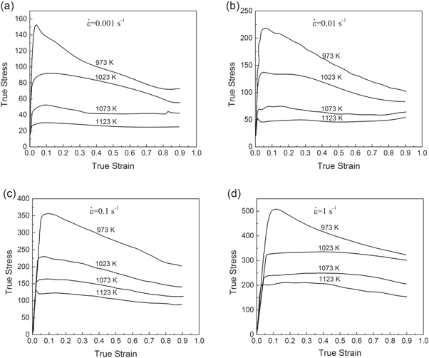
Figure 2. The true strain-stress curves of Ti-55 531 alloy at the strain rate of: (a) 0.001 s−1; (b) 0.01 s−1; (c) 0.1 s−1; (d) 1 s−1.
Download figure:
Standard image High-resolution image3.2. BP-ANN model construction
The BP-ANN has been used to compute the constitutive relationships between experimental data and predicted data with high precision [21]. As shown in figure 3, the BP-ANN has a structure consisting of input layer, hidden layer and output layer. The outside signals (strain, strain rate and temperature) were received by input layer and delivered to hidden layer which can provide complex network to train and mimic the non-linear relationship between input layer and output layer [22]. Subsequently, processed signals (stress) were generated and outputted by output layer. For the simple and quick computation, the input and output signals should be normalized and non-normalized respectively. The normalized values were chosen from 0 to 1 in previous report [23]. In this work, to make the calculation more convenient, the normalized values were determined from −1 to 1 using the default settings of ANN. The values of input signals were normalized by the following equation:

where X is original data,  is the normalized result of X, Xmin is the minimum value of original data and Xmin is the maximum value of original data.
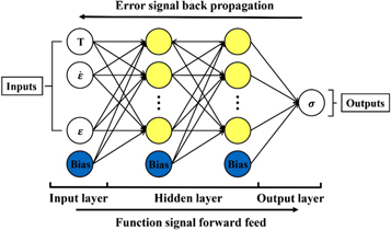
Figure 3. The schematic of the back-propagation artificial neural network architecture.
Download figure:
Standard image High-resolution imageTo achieve optimal accuracy, the number of hidden layers was determined to be two according to previous report [24] which choose two hidden layers after comparing with single hidden layer. Besides, it is very important to chose suitable neurons for the hidden layers. Too many or too few neurons may both lead the training processes insufficient. Thus, a trial-and-error procedure was provided to determine the neuron number: two neurons were taken into the training at the beginning and more neurons were added one-by-one. The sum square error (SSE) [25] (expressed as equation (2)) between experimental and predicted values was introduced to evaluate the accuracy of the trained ANN model [22]. Generally, lower SSE-value in ln scale means high accuracy of the model. As shown in figure 4, the SSE-value reaches a bottom value at 12 neurons, which indicates that the best accuracy in the trial-and-error procedure is achieved.

where Ei is the value of experiment, Pi is the value of prediction, and N is the total number of values.

Figure 4. The sum square error values of two hidden layers with different neurons.
Download figure:
Standard image High-resolution imageFigure 5 shows the comparisons between the experiment data of Ti-55531 alloy and the predicted data based on BP-ANN at different conditions. In figure 5, the hollow dots are predicted data based on the developed model and the red points are the limited input training data. It can be seen that, for most curves, the training data were picked from the strain value of 0.1 to 0.9 with the interval of 0.1 and the predicted data were chosen from the strain value of 0.05 to 0.85 with the interval of 0.1. As an exception, no data from 0.001 s−1 and 973 K and 0.1 s−1 and 1073 K was taken into training and these two curves were totally predicted. Most of all, the prediction points are nearly on the curves of experimental results, which means that the developed model is capable to simulate the curve types corresponding to different microstructural mechanism including working hardening, DRX, DRV and their interactions with each other. Based on the good agreement of experimental results and predicted data, it can be concluded that this developed model is capable to predict the flow stress of Ti-55531 alloy accurately and efficiently.

Figure 5. The predicted data based on BP-ANN at the strain rate of: (a) 0.001 s−1; (b) 0.01 s−1; (c) 0.1 s−1; (d) 1 s−1.
Download figure:
Standard image High-resolution image3.3. Modelling of Arrhenius constitutive
As a very classical constitutive model, the Arrhenius equation (as show in equation (3)) is widely applied to express the relationships of flow stress, temperature and strain rate of alloys. [13, 26, 27]

where
and where  Q, R, T, σ are the strain rate, activation energy, gas constant, absolute temperature and flow stress, respectively. A, A1, A2, α, β, n and n1 are material constants, and α = β/n1.
Besides, the Zener-Hollom parameter (Z) is introduced to present the effects of deformation parameters on deformation behaviors. It is expressed in an exponent-type equation as following [28]:

Based on equations (3) and (4), the function could be denoted as:

On the basis of the solution processes of the material constants used by Xia et al [29]. The values of α, Q, lnA, n from the strain of 0.05 to 0.9 with the interval of 0.05 have been determined. Then, the determined values were fitted by the sixth order polynomial functions in equation (6). The relationships between true strain and constants including α, lnA, n, Q by polynomial fit were shown in figure 6. In figure 6, the adjusted coefficients of determination between the fitted curves and determined α, lnA, n, Q are 0.9996, 0.9994, 0.9729 and 0.9993 respectively. The corresponding coefficients are listed in table 2.


Figure 6. The relationships between true strain and (a) α, (b) lnA, (c) n, (b) Q by polynomial fit.
Download figure:
Standard image High-resolution imageTable 2. The coefficients of the sixth order polynomial functions.
| α | lnA | n | Q | ||||
|---|---|---|---|---|---|---|---|
| B0 | 0.006 56 | C0 | 33.563 11 | D0 | 4.191 00 | E0 | 321.427 11 |
| B1 | 0.000 62 | C1 | 86.997 58 | D1 | −18.139 34 | E1 | 863.168 00 |
| B2 | −0.002 53 | C2 | −858.2454 | D2 | 116.778 94 | E2 | −8168.501 23 |
| B3 | 0.027 99 | C3 | 2743.568 07 | D3 | −380.882 43 | E3 | 25 975.399 69 |
| B4 | −0.058 83 | C4 | −4188.849 56 | D4 | 645.120 00 | E4 | −39 715.949 46 |
| B5 | 0.057 95 | C5 | 3055.621 66 | D5 | −542.497 76 | E5 | 29 129.572 45 |
| B6 | −0.022 46 | C6 | −850.188 73 | D6 | 179.259 36 | E6 | −8176.625 13 |
According to equations (4) and (5), the solution expression for stress can be expressed as:

where g(ε), f(ε), j(ε) and h(ε) are the projection functions of α, A, Q and n, respectively.
So far, the stress predicted values based on developed Arrhenius model can be obtained by applying the material constants into equation (7). The predicted values based on developed Arrhenius model at different deformation conditions are shown in figure 7. It can be seen that, to some extent, the predicted values are accurate and the share the similar features with experimental results.

Figure 7. The predicted values based on developed Arrhenius model at the strain rate of: (a) 0.001 s−1; (b) 0.01 s−1; (c) 0.1 s−1; (d) 1 s−1.
Download figure:
Standard image High-resolution image3.4. Comparison of the prediction accuracy between BP-ANN model and Arrhenius model
As mentioned in Part 3.2, no data from 0.001 s−1 and 973 K and 0.1 s−1 and 1073 K was taken into training and 18 points for each of these deformation conditions were predicted. Thus, to assess the prediction accuracy of the two models, the predicted results at these two deformation conditions predicted by the two models were taken into comparison using the relative error calculated by equation (8).

where Ei is the experimental result and Pi is the predicted result.
The relative errors of the predictions of the two models under the condition of 973 K and 0.001 s−1 and 1073 K and 0.1 s−1 are listed in table 3. In table 3, the relative errors of predicted results by Arrhenius model vary from −10.87% to 11.84%. As distinct comparisons, the relative errors of BP-ANN model vary from −3.63% to 6.87%. To analyze statistically, the relative errors distribution histograms of the two models were plotted as shown in figure 8. Meanwhile, the mean value (μ) and the standard deviation (ω) were introduced to evaluate the concentration degree of relative errors distribution. Statistically speaking, smaller values of μ and ω close to zero mean better errors distribution, which indicate better prediction accuracy. For BP-ANN model, the μ-value and the ω-value were calculated to be 1.4714% and 2.2271% according to equation (9) and equation (10), respectively, while for Arrhenius model, the corresponding values were −1.2213% and 5.3641%, respectively. It is obvious that the concentration degree in the low relative error values field (near zero) of BP-ANN model is higher, which further indicates the better prediction capability of this model.


Where δi is the relative error.
Table 3. The relative errors of the predicted results by the BP-ANN model and Arrhenius constitutive model under the condition of 973 K and 0.001 s−1 and 1073 K and 0.1 s−1.
| True Stress (MPa) | Relative error (%) | ||||||
|---|---|---|---|---|---|---|---|
| Temperature (K) | Strain rate (s−1) | True Strain | Experimental | BP | Equation | BP | Equation |
| 973 | 0.001 | 0.05 | 150.3283 | 140.0000 | 132.5232 | 6.87 | 11.84 |
| 0.10 | 137.6625 | 135.0000 | 137.7892 | 1.93 | −0.09 | ||
| 0.15 | 130.8392 | 128.0000 | 135.0674 | 2.17 | −3.23 | ||
| 0.20 | 123.9074 | 122.0000 | 127.9562 | 1.54 | −3.27 | ||
| 0.25 | 115.6022 | 112.7965 | 119.9472 | 2.43 | −3.76 | ||
| 0.30 | 109.7832 | 107.0065 | 112.5671 | 2.53 | −2.54 | ||
| 0.35 | 104.3758 | 102.1358 | 106.2062 | 2.15 | −1.75 | ||
| 0.40 | 100.2436 | 99.9703 | 100.8487 | 0.27 | −0.61 | ||
| 0.45 | 97.288 03 | 96.1017 | 96.2390 | 1.22 | 1.08 | ||
| 0.50 | 93.8188 | 91.8649 | 91.9797 | 2.08 | 1.96 | ||
| 0.55 | 90.089 81 | 89.3664 | 87.8510 | 0.80 | 2.49 | ||
| 0.60 | 86.699 59 | 84.5607 | 83.7323 | 2.47 | 3.42 | ||
| 0.65 | 82.4068 | 80.3274 | 79.6456 | 2.53 | 3.35 | ||
| 0.70 | 78.201 22 | 76.5234 | 75.7988 | 2.14 | 3.07 | ||
| 0.75 | 75.143 59 | 73.0068 | 72.4306 | 2.84 | 3.61 | ||
| 0.80 | 72.595 63 | 69.6386 | 69.8585 | 4.08 | 3.78 | ||
| 0.85 | 72.017 25 | 71.2736 | 68.5897 | 1.04 | 4.76 | ||
| 0.90 | 72.723 65 | 72.7490 | 68.8427 | −0.04 | 5.33 | ||
| 1073 | 0.1 | 0.05 | 162.9977 | 159.8255 | 151.4557 | 1.95 | 7.08 |
| 0.10 | 164.1686 | 165.5622 | 158.5896 | −0.85 | 3.40 | ||
| 0.15 | 162.2951 | 167.9215 | 161.5061 | −3.46 | 0.49 | ||
| 0.20 | 161.5925 | 167.2418 | 161.1295 | −3.50 | 0.28 | ||
| 0.25 | 158.3138 | 164.0540 | 159.1797 | −3.63 | −0.55 | ||
| 0.30 | 154.6838 | 159.0280 | 156.6391 | −2.81 | −1.27 | ||
| 0.35 | 152.3419 | 152.8453 | 153.8963 | −0.33 | −1.02 | ||
| 0.40 | 147.6581 | 146.0694 | 151.0752 | 1.08 | −2.31 | ||
| 0.45 | 142.9742 | 139.0878 | 148.1462 | 2.72 | −3.62 | ||
| 0.50 | 137.3536 | 132.1415 | 144.9852 | 3.79 | −5.56 | ||
| 0.55 | 133.7237 | 130.4087 | 141.5639 | 2.48 | −5.87 | ||
| 0.60 | 128.8056 | 124.0838 | 138.0299 | 3.67 | −7.16 | ||
| 0.65 | 123.6534 | 118.4187 | 134.5340 | 4.23 | −8.80 | ||
| 0.70 | 120.6089 | 118.7182 | 131.3572 | 1.57 | −8.91 | ||
| 0.75 | 117.4473 | 115.3024 | 128.6839 | 1.83 | −9.56 | ||
| 0.80 | 114.1686 | 113.4546 | 126.5316 | 0.63 | −10.83 | ||
| 0.85 | 112.5293 | 110.3701 | 124.7627 | 1.92 | −10.87 | ||
| 0.90 | 113.1148 | 110.1128 | 122.5498 | 2.65 | −8.35 | ||

Figure 8. The relative errors distribution histograms of (a) BP-ANN model and (b) the Arrhenius model.
Download figure:
Standard image High-resolution imageFor further evaluation, as two important statistical indicators, correlation coefficient (R) (expressed as equation (11)) and average absolute relative error (ARRE) (expressed as equation (12)) were introduced to assess the predication capability of the two models [30]. It is known that the R-values close to −1, 0 and 1 are corresponding to strong negative relationship, no relationship and strong positive relationship, respectively. Also, smaller absolute AARE-value indicates the smaller difference between predicted values and experimental values.


Where Ei is the value of experiment and Pi is the value of prediction.  and
and  are the corresponding mean values, and N is the number of data.
Figure 9 shows the correlation relationships between the values of experiment and prediction by the two models. The R-values of the BP-ANN model and the Arrhenius model are 0.9949 and 0.9761 respectively and the AARE-values of BP-ANN model and Arrhenius model are 2.2836% and 23.4527% respectively. So far, the prediction capability of BP-ANN model has been proved to be better than Arrhenius model.

Figure 9. The correlation relationships between the values of experiment and prediction by: (a) BP-ANN model, (b) the Arrhenius constitutive model.
Download figure:
Standard image High-resolution image3.5. Extension capability of the developed BP-ANN model
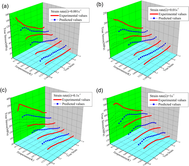
According to the results and discussion above, the reliability and accuracy of the developed BP-ANN model has been proved. As shown in figure 10, the flow stress of Ti-55531 alloy at the temperatures of 998, 1058, 1098, 1158 K and the strain rates of 0.001, 0.01, 0.1, 1 s−1 were predicted by the developed BP-ANN model. In figure 10, the red curves represent the 3D curves of experimental results and the blue square dots represent the predicted points. Also, among the extended curves, some curve types corresponding to different microstructural mechanism such as DRX (0.1 s−1 and 998 K), WH (0.001 s−1 and 998 K) and DRV (0.01 s−1 and 1158 K) can be observed, which validates the applicability of BP-ANN model in predicting the flow curves of Ti-55531 alloy outside the experimental conditions. It is well known that stress-strain curves are the fundamental data used in the finite element simulation during hot deformation. With high accuracy predicted expanded data and basic experimental data, more accurate finite element simulation of a certain forming process could be achieved.
Figure 10. The 3D plot of flow stress as function of strain and temperature at the strain rate of: (a) 0.001 s−1; (b) 0.01 s−1; (c) 0.1 s−1; (d) 1 s−1.
Download figure:
Standard image High-resolution image
4. Conclusions
The BP-ANN model and the Arrhenius model for Ti-5Al-5Mo-5V-3Cr-1Zr have been constructed based on the experimental results from hot compression tests in a temperature range of 973 K to 1123 K and a strain rate of 0.001 to 1 s−1. The constructed models were used to predict the stress values and compared with each other. The following conclusion were drawn:
- (1)An Arrhenius model was developed and the material constants including α, A, Q and n at different conditions were calculated to help predicting the flow curves of Ti-5Al-5Mo-5V-3Cr-1Zr. Good correlations between experimental values and predicted values could be observed on the basis of the results.
- (2)The relative error and the standard deviation for BP-ANN model were calculated to be 1.4714% and 2.2271%, while for Arrhenius model, the corresponding values were −1.2213% and 5.3641%, respectively. Besides, the correlation coefficients of BP-ANN model and Arrhenius model are 0.9949 and 0.9761 respectively. The average absolute relative error for BP-ANN model and Arrhenius model are 2.2836% and 23.4527% respectively.
- (3)The flow curves were extended on the basis of the BP-ANN model, which is believed to be helpful to achieve high accuracy in finite element simulation.
Acknowledgments
This work was supported by Chongqing higher school talented person supportive program (800213).