


Abstract
Phase synchronisation in multichannel electroencephalography (EEG) is known as the manifestation of functional brain connectivity. Traditional phase synchronisation studies are mostly based on time average synchrony measures, and hence do not preserve the temporal evolution of the phase difference. Here we propose a new method to show the existence of a small set of unique phase synchronised patterns or 'states' in multi-channel EEG recordings, each 'state' being stable of the order of ms, from typical and pathological subjects during face perception tasks. The proposed methodology bridges the concepts of EEG microstates and phase synchronisation in the time and frequency domain, respectively. The analysis is reported for four groups of children including typical, autism spectrum disorder, low and high anxiety subjects—a total of 44. In all cases, we observe consistent existence of these states—termed as synchrostates—within specific cognition-related frequency bands (beta and gamma bands), though the topographies of these synchrostates differ for different subject groups with different pathological conditions. The inter-synchrostate switching follows a well-defined sequence capturing the underlying inter-electrode phase relation dynamics in a stimulus- and person-centric manner. Our study is motivated by the well-known EEG microstate exhibiting stable potential maps over the scalp. However, here we report a similar observation of quasi-stable phase synchronised states in multichannel EEG. The existence of the synchrostates coupled with their unique switching sequence characteristics could be considered as a potentially new field over contemporary EEG phase synchronisation studies.
Export citation and abstract BibTeX RIS
1. Introduction
The intrinsic organization of the human brain could be viewed as a dynamic network, changing its configuration at a sub-second level temporal scale depending upon a given cognitive task. Phase synchronisation dynamics between different cortical areas is fundamental to formulate a mathematical representation of such dynamically reconfiguring functional networks (Engel et al 2001, Fell and Axmacher 2011). Electroencephalography (EEG) is an effective tool for studying such phase synchronisation owing to its high temporal resolution, and has been applied extensively in the past (Mulert et al 2011, Razavi et al 2013) for studying such phenomena, unearthing useful information about cognitive processes.
Traditionally, EEG-based synchronisation analysis is mostly carried out at a time scale of the order of seconds, apart from the well-known microstate analysis (Koenig et al 2002), where the scalp level distribution of the electric field was studied at ms resolution level. Recently, during a visual perception task, it has been shown that at ms time scales, there exists a small set of unique phase synchronised patterns, each being stable of the order of ms, and then abruptly switching from one to another (Jamal et al 2015). These quasi-stable phase difference patterns are termed as synchrostates. It was first observed in a single adult subject (Jamal et al 2013a, 2013b) and later in group average of typically developing as well as autistic children (Jamal et al 2013a, 2013b) in their respective EEG γ-bands. Subsequently functional connectivity networks were formulated from these γ-band synchrostates, and then applying graph theoretic characterization of them it was shown possible to classify autistic and typically developing population with high accuracy (Jamal et al 2014). This indicates towards the possibility of using synchrostates as a new way for functional connectivity network analysis in different populations. However the pertinent question is whether the synchrostates consistently exist in individual subjects in the cognition related bands (β and γ), and if so, how much inter-subject variability could be expected with respect to the population average, as this is fundamental in ascertaining the possibility of classifying an individual's pathological conditions using graph theoretic characterization of a functional brain network formed from the synchrostates.
Therefore, the main aims of this paper are: (1) systematically exploring the existence and nature of synchrostates in both the β and γ bands for individuals not only belonging to typically developing but also from a pathological population, (2) studying the variability of synchrostates with respect to the number of EEG electrodes used, (3) to elaborate the method of synchrostate formulation in a step-by-step fashion, showing how this method combines the existence of time-domain discrete state concepts of microstates and frequency domain phase synchronisation analysis. The cognitive task selected for our exploration is a set of face-perception tasks where three types of face-perception related stimuli were given to four groups of children—with typical development, diagnosed with autism spectrum disorder (ASD), and with high- and low-anxiety scores. Since β and γ bands have consistently shown increased synchrony during face-perception tasks (Rodriguez et al 1999, Uhlhaas et al 2009, Kottlow et al 2012) and prominent response during visual stimuli in general (Wróbel 2000, Lachaux et al 2005), we mainly concentrated on analysing these two bands. Our exploration showed: (1) the synchrostates exist in individual subjects consistently in both the β and γ bands and are usually bounded between 3 and 7, whereas in the low frequency bands (θ, α) there is no consistent existence of synchrostates; (2) synchrostates exhibit qualitatively similar behaviour to that of the EEG microstates in terms of their temporal stability and switching characteristics; (3) although the general set of synchrostate topographies are similar for a subject group corresponding to different visual perception stimuli, the actual time-courses of the inter-synchrostate switching sequence are markedly different, indicating stimulus-specific dynamics even within the broad category of visual perception tasks; and (4) using fewer electrodes results in greater variability in the number of synchrostates with respect to the corresponding population average, whereas a high density EEG gives more consistent results.
In addition, here we define all the synchrostates according to their topographical distribution of average phase difference over the scalp and reassign the class labels of similar topoplots with a state label which has been shown to vary little across different stimuli within the same population. We also observed that these synchrostates have different configurations in the β and γ bands as well as across different subject groups. Also, in order to quantify the qualitative behaviour of the synchrostate transitions, we calculated the probability of self-transition, implying the degree of relative stability of these states in each combination of stimulus, population and frequency band.
2. Method
2.1. Background
Typical synchronisation can be studied from EEG signals in two domains, i.e. time and frequency. The work reported in (Lehmann et al 1987, Koenig et al 2014) considered brain electric states with consistent scalp electric field topography, and their sequence which led to what is commonly known as EEG microstates. Its most important characteristic is that the topography does not change randomly or continuously over time, but exhibits quasi-stable behaviour in the order of 80–120 ms; and abruptly switches from one topography to another—the number of unique topographies being small (typically 3–10) (Koenig et al 2002). Another way to study the synchronisation phenomenon is in the frequency domain. This is led by the assumption that if two points (i.e. two EEG electrode sites) are in coherence (i.e. maintaining constant phase relationship over time), they can be considered as functionally synchronised or connected (Fries et al 2001). Phase coupling has been studied in patients with mental disorders (Mulert et al 2011, Razavi et al 2013) and the merits of synchrony analysis have been found in the understanding of neurodevelopmental disorders (Uhlhaas et al 2008). Since the method for coherence analysis, like global field synchronisation (Kottlow et al 2012), uses Fourier transform, inherently it does not preserve the temporal information of synchronisation. This methodology was later modified by several researchers by using continuous wavelet transform (CWT) and Hilbert transform (HT) to compute the phase in transformed domains and for deriving the associated synchronisation indices from the coherence values thus obtained. The mean phase coherence measure (Mormann et al 2000) computes the synchronisation over the whole time series and therefore gives an average measure of synchronisation for the whole signal span. The phase locking value, although it varies with time, measures the inter-trial variability of phase difference (Rodriguez et al 1999) rather than temporal variability. Additionally, various other measures of phase synchronisation have been reported in (Quiroga et al 2002). Although useful, such approaches only give an insight into the phase synchronisation in a time-averaged way over all the frequency bands, rather than capturing the true picture of the temporal or transient evolution of phase synchrony in a band-specific way. On the other hand, in principle, CWT and HT both being time–frequency transform methods, have the potential to describe the temporal evolution of phase synchronisation at a sub-second resolution level, which could be more informative to understand the dynamics of the synchronisation phenomena from the onset of a given stimulus until the end of the corresponding cognitive action.
As evident from the foregoing discussion, the existing frequency domain methods compute the phase synchronisation over the entire post stimulus segment of the signal and therefore are unable to retain the transient information at finer temporal granularity, whereas the microstate method finds the unique electric potential patterns and their transients during the execution period of the task (Gianotti et al 2008). Ito et al studied the dynamics of spontaneous transitions between globally phase-synchronised states in the alpha band EEG activity (Ito et al 2007). Their method was applied to explore the phase dynamics of individuals with cerebral palsy (Daly et al 2014). The technique proposed in these articles investigates phase dynamics by segmenting the relative phase patterns into global phase pattern states by thresholding and using a criterion called the instantaneous instability index (III). The GPS pattern vectors are then clustered into six centroids. Here we propose a slightly different approach for studying the dynamical evolution of phase patterns by using intrinsic optimization criterion in the k-means clustering for segmentation of the images to form compact clusters or states without any prior thresholds. In this paper we merge two concepts, i.e. the concept of temporal switching (transient behaviour) of stable states along with the band specific phase locking by considering a joint time–frequency representation of the EEG signal.
2.2. Data and pre-processing
The data analysis was conducted with four distinct samples of children: (1) with typical development, (2) diagnosed with ASD, (3) diagnosed with high-anxiety and (4) with low-anxiety. More specifically, we have used the data acquired during the experiments described in (Apicella et al 2013) and (Chronaki 2011). For more information regarding the data used in this study please refer to the supplementary material, available online. The main characteristics of these four populations are summarized in table 1.
Table 1. Summary of the subject group and presented stimuli.
| Group number | Group type | Number of subjects | Age range | Number of EEG channels | Stimuli presented (types of faces) |
|---|---|---|---|---|---|
| I | Typical development | 12 | 6–13 | 128 | Happy, fear, neutral |
| II | ASD | 12 | 6–13 | 128 | Happy, fear, neutral |
| III | High-anxiety | 10 | 6–12 | 30 | Happy, angry, neutral |
| IV | Low-anxiety | 10 | 6–12 | 30 | Happy, angry, neutral |
For groups I and II the data was acquired using a 128 channel EEG system and was segmented into a 1000 ms epoch with 150 ms baseline and 850 ms post-stimulus response. Epochs over a threshold of 200 μV were rejected as artefacts. Data was baseline corrected and band-pass filtered from 0.5 to 50 Hz for removing low-frequency drifts and high-frequency measurement noise using a 5th order Butterworth filter. On the other hand, for groups III and IV a 30 channel EEG system was used for data acquisition and data was epoched at 100 ms pre-stimulus to 1000 ms post-stimulus. Collected data was band-pass filtered in the range 0.1–70 Hz to eliminate the drift and noise as done in the former case. These pre-processed EEG signals were then transformed in the time–frequency domain using CWT, with particular focus on the two bands of interest viz. β (13–30 Hz) and γ (30–50 Hz). Only the response of the frequencies in these two bands of interest is then used for further processing. Being band-specific, this processing step allows us to compare the response of the signals across all the groups on a uniform platform, although they were acquired with different instruments. The studies in (Nunez et al 1997, Schiff 2005) point out that the use of average reference for calculating coherency is a good compromise against the effects and noise introduced by the reference electrode. In our study, all the signals were re-referenced to average reference data (average across all channels) and then were used for our calculation. The different data collection protocols adopted for groups I–II; and III–IV allows us to explore the effect of variability in the number of EEG electrodes.
2.3. Computation of time-dependent phase difference topography
It has been observed by researchers that the spectral power of different EEG bands significantly changes depending upon the stimulus given (Boiten et al 1992). As a consequence it may be assumed that the temporal stability of instantaneous phase difference topographies and hence the overall synchronisation pattern may manifest differently in different EEG bands. Therefore it appears to be more logical to study the synchronisation phenomenon in a band-specific way. Since CWT decomposes a signal to different scales (equivalent frequencies) at each time instant, it is possible to study the temporal evolution pattern of phase difference topographies for an isolated frequency band of interest. Therefore in our analysis we used CWT as the main analysis tool, more precisely, we have used a complex Morlet basis function as shown in (1) for computing the CWT of the EEG data

where,  denote the bandwidth parameter and the centre frequency respectively. For our purpose we considered
  and
and  .
.
Considering N number of EEG channels placed over the scalp and  be the EEG signals acquired at the respective channels, application of complex Morlet CWT on
  results in a complex time series
  at the wavelet scale a at time t.
  can be converted to a function of frequency and time
  using the following relation (Addison 2010) in (2)

where δ and f are the sampling period and the approximate pseudo-frequency, i.e. the frequencies corresponding to the scales, respectively. Subsequently, the instantaneous phase φi(f, t) of Wi(f, t) can be computed as (3)

Im[Wi(f, t)] and Re[Wi(f, t)] are the imaginary and the real part of Wi(f, t) respectively. Consequently, the instantaneous phase difference  between the channels i and j can be given by (4)

Computation of  at a time instant t1 and frequency f1 for
  yields a symmetric square matrix
 ![$\left[\Delta \varphi ({f}_{1},\;{t}_{1})\right]$](https://content.cld.iop.org/journals/2057-1976/1/1/015002/revision1/bpex516831ieqn12.gif) that describes the pairwise relationship of phase difference at the frequency f1 for all the EEG channels at t1 time instant as shown in figure 1. For computing the average response within a subject group the individual
that describes the pairwise relationship of phase difference at the frequency f1 for all the EEG channels at t1 time instant as shown in figure 1. For computing the average response within a subject group the individual  were averaged over all the subjects to get the average wavelet response for the group under consideration. Therefore, if the frequency band of interest
  is spanned over the frequencies
  then the instantaneous phase difference matrix for B at time t as shown in figure 2 can be formulated as (5)–(6)


where  is the (i, j)th element of the matrix
 ![$\left[\Delta {\varphi }_{B}(t)\right]$](https://content.cld.iop.org/journals/2057-1976/1/1/015002/revision1/bpex516831ieqn17.gif) and
and  is the (i, j)th element of
 ![$\left[\Delta {\varphi }_{{f}_{k}}(t)\right].$](https://content.cld.iop.org/journals/2057-1976/1/1/015002/revision1/bpex516831ieqn19.gif) Subsequently,
Subsequently, ![$\left[\Delta {\varphi }_{B}(t)\right]$](https://content.cld.iop.org/journals/2057-1976/1/1/015002/revision1/bpex516831ieqn20.gif) can be computed at different time instants
can be computed at different time instants  resulting in a set of such matrices
 ![$\left[\Delta {\varphi }_{B}\left({t}_{1}\right)\right],\;\left[\Delta {\varphi }_{B}\left({t}_{2}\right)\right],\cdots ,\;\left[\Delta {\varphi }_{B}\left({t}_{n}\right)\right]$](https://content.cld.iop.org/journals/2057-1976/1/1/015002/revision1/bpex516831ieqn22.gif) like that shown in figure 3, which describes the complete picture of temporal evolution of the phase difference from the onset of a stimulus until the end of the corresponding action in the particular frequency band B over all the EEG channels on the scalp. The whole process is pictorially depicted in figures 1–3. As evident, due the high dimensionality of the clustering problem, a simple cluster discrimination through a scatter plot is not possible in the present study. In our clustering framework, at each time instant the dimension of the feature space, denoting all possible cross-electrode phase information, becomes N2 and the clustering algorithm considers the evolution of each element
like that shown in figure 3, which describes the complete picture of temporal evolution of the phase difference from the onset of a stimulus until the end of the corresponding action in the particular frequency band B over all the EEG channels on the scalp. The whole process is pictorially depicted in figures 1–3. As evident, due the high dimensionality of the clustering problem, a simple cluster discrimination through a scatter plot is not possible in the present study. In our clustering framework, at each time instant the dimension of the feature space, denoting all possible cross-electrode phase information, becomes N2 and the clustering algorithm considers the evolution of each element  along time.
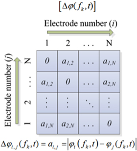
Figure 1. The structure of the phase difference matrix at frequency fk at time t.
Download figure:
Standard image High-resolution image
Figure 2. Computation principle of a band-specific phase difference matrix.
Download figure:
Standard image High-resolution image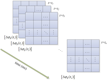
Figure 3. Computation of band-specific phase difference matrix from the onset of a stimulus until the end of the desired time window.
Download figure:
Standard image High-resolution image2.4. Clustering of phase difference matrices into a unique set of 'states'
Once all the cross-electrode phase difference matrices for a particular band are formulated over the entire duration of a specified time interval—in our case, we are interested to see the temporal evolution of these topographies at subsecond order time interval—the next pertinent question is whether there exists any unique 'spatio-temporal patterns' of phase difference topographies during the execution of the cognitive task. The first step for that is to identify all 'possibly unique' topographies over the entire time duration of interest. A certain class of pattern recognition techniques could be employed for this purpose. The k-means clustering is one such unsupervised pattern recognition technique. For a given dataset X, ![$X=\left\{{x}_{p}\right\},p\in \left[1,\cdots ,P\right],$](https://content.cld.iop.org/journals/2057-1976/1/1/015002/revision1/bpex516831ieqn24.gif) assuming the number of underlying clusters is known, the k-means algorithm iteratively minimizes a cost function given below (7)
assuming the number of underlying clusters is known, the k-means algorithm iteratively minimizes a cost function given below (7)

where ![$\theta ={\left[{\theta }_{T1}\ldots \;{\theta }_{Tm}\right]}^{T},$](https://content.cld.iop.org/journals/2057-1976/1/1/015002/revision1/bpex516831ieqn25.gif)
 is the Euclidean distance,
  is the centre of a cluster and
  if xp lies closest to θq; 0 otherwise. Initially k centroids are defined and depending on how near the data vector is to the centroids, it is assigned to a class. The k centroids are iteratively recalculated and the data is reassigned to these new centroids until the data vectors from X form compact clusters and the cost function J is minimized. Initially a range [mmin, mmax] is defined for possible clusters m for the dataset X. The k-means clustering runs n (n random initializations) times for each m within that range and for every n runs the minimum value of the cost function Jm (as shown in (7)) is calculated and stored. The cost function Jm essentially indicates the sum of distances of the data-points from the nearest cluster mean when m clusters are considered. The value of Jm is dependent on the number of clusters and also the dataset under consideration, whereas a high value of Jm represents a less compact cluster. Thus we search for a 'knee' in the plot of Jm against m as an indication of the number of optimal clusters underlying the data. If the plot of Jm against m shows a significant 'knee' at m = m1 (say) then it signifies that the number of optimum clusters underlying the dataset X is likely to be m1. To be noted that in the plot of Jm versus m it is typical to have multiple such knees as m varies within its selected range. In cases, where there is an increase in the Jm value, it indicates that the distance between all the data points with respect to the nearest mean of clusters has increased. This increase could be due to the splitting of large compact clusters into several smaller ones, caused by increasing the value of m. In such a case, one needs to consider the earliest and the most prominent knee as the characteristic knee and the corresponding m as the underlying number of clusters as it explains the dataset with minimum complexity. Another important point to note that the absolute value of Jm in the plot of Jm against m is not important but the value of m at which Jm attains minimum value (the significant knee) is the important parameter indicating the number of underlying clusters. This method is also known as the incremental k-means or elbow method and is widely used to find the optimum number of clusters in a given data-set.
In a higher dimensional feature space, the landscape of the cost function J(θ) may have multiple local minima and there is small probability of finding a higher value of the cost function if a local minima has been found by the optimization process. Since the k-means clustering has the problem of getting trapped to local minima, it should be run multiple times with different initialization of the cluster means and the best result with the minimum value of the cost function should be considered. Therefore in our method, the best-results of the k-means algorithm for each choice of k is considered out of n = 10 different random initializations of the cluster means. This way the incremental k-means plots the best cost function to obtain the Jm as also suggested in (Theodoridis et al 2010).
The unsupervised learning technique adopted here is based on the concept of hard clustering, i.e. a single data-point corresponding to each time instant should belong to one of the clusters, because in a temporal resolution of a millisecond, we assume that the brain stays only in one state. Other paradigms of soft clustering like fuzzy c-means or similar methods (Dimitriadis et al 2013) where a single data-point can be associated with more than one cluster according to its degree of associativity with different classes, could also be applied to the present problem.
In our case, X is the dataset of all pairwise EEG instantaneous phase differences ![$\left[\Delta {\varphi }_{B}\left({t}_{1}\right)\right],\;\left[\Delta {\varphi }_{B}\left({t}_{2}\right)\right],\;\mathrm{..}.,\;\left[\Delta {\varphi }_{B}\left({t}_{n}\right)\right],$](https://content.cld.iop.org/journals/2057-1976/1/1/015002/revision1/bpex516831ieqn29.gif) as a function of time. We clustered the dataset X along time t, for a chosen frequency band B, to find out unique phase difference patterns. The algorithm yields k centroids,
as a function of time. We clustered the dataset X along time t, for a chosen frequency band B, to find out unique phase difference patterns. The algorithm yields k centroids,  for each cluster or state and a vector of length n with the corresponding state or cluster labels for each
 ![$\left[\Delta {\varphi }_{B}(t)\right]$](https://content.cld.iop.org/journals/2057-1976/1/1/015002/revision1/bpex516831ieqn31.gif) for every time instance over which we clustered. The centroids hold average information for each of the clustered states whereas the cluster labels signify when in time each state has occurred. Once the phase-difference matrices are uniquely clustered over different time instances, the centroids are translated into corresponding colour-coded head-map topographies following arbitrary colour coding convention. This is done by first calculating the average phase difference seen at a particular electrode with respect to the rest of the electrodes i.e. taking the row-wise average of
for every time instance over which we clustered. The centroids hold average information for each of the clustered states whereas the cluster labels signify when in time each state has occurred. Once the phase-difference matrices are uniquely clustered over different time instances, the centroids are translated into corresponding colour-coded head-map topographies following arbitrary colour coding convention. This is done by first calculating the average phase difference seen at a particular electrode with respect to the rest of the electrodes i.e. taking the row-wise average of ![$[\Delta {\varphi }_{B}\left(t\right)]$](https://content.cld.iop.org/journals/2057-1976/1/1/015002/revision1/bpex516831ieqn32.gif) and considering it as the average phase difference at that electrode index corresponding to the considered row and assigning a particular colour corresponding to the numerical value of that phase difference and finally transforming it to a contour plot. Such head-map topographies give a visual representation of the distribution of average phase differences between different regions of the brain over the scalp. Note that these plots should not be viewed or compared to the typical EEG potential plots or the power spectrum plot typically generated in quantitative EEG (qEEG) analysis. Here the plots show the gross phase difference between different electrodes over the scalp over a particular time window. Higher numerical values represent a greater gross phase difference of the electrode with all the other electrodes and low values indicate that the electrode has a relatively lower phase difference than all the other electrodes in that configuration. We term the set of topography clusters identified using k-means algorithm as synchrostates. The state labels are used to construct a transition plot to illustrate the switching sequence of the synchrostates over the time of the EEG recording. This is simply done by plotting the time labels yielded by the clustering algorithm.
and considering it as the average phase difference at that electrode index corresponding to the considered row and assigning a particular colour corresponding to the numerical value of that phase difference and finally transforming it to a contour plot. Such head-map topographies give a visual representation of the distribution of average phase differences between different regions of the brain over the scalp. Note that these plots should not be viewed or compared to the typical EEG potential plots or the power spectrum plot typically generated in quantitative EEG (qEEG) analysis. Here the plots show the gross phase difference between different electrodes over the scalp over a particular time window. Higher numerical values represent a greater gross phase difference of the electrode with all the other electrodes and low values indicate that the electrode has a relatively lower phase difference than all the other electrodes in that configuration. We term the set of topography clusters identified using k-means algorithm as synchrostates. The state labels are used to construct a transition plot to illustrate the switching sequence of the synchrostates over the time of the EEG recording. This is simply done by plotting the time labels yielded by the clustering algorithm.
3. Results
As mentioned previously, we restrict our study only in the β and γ band since research indicated that they are directly related to the cognitive task related to face perception (Wróbel 2000, Lachaux et al 2005). We present the results in two steps: first as a population average and then for individual subjects belonging to a population. To study the population average we first formulate the average phase difference matrix for each subject by taking the mean of the phase difference matrices across all trails. Then we take an average of the phase matrices of each subject belonging to that population at every time instant and invoke k-means clustering on that set of average matrices as described in sections 2.2 and 2.3. In essence this gives a general picture of temporal evolution of phase relationship between different electrode sites for a specific population. Our exploration shows that the cost function for clustering does not fall arbitrarily with the increase in the number of clusters, confirming the existence of a finite number of compact underlying clusters or states during the whole time-course of the EEG data. The detailed results for the individual groups are furnished in the following subsections.
3.1. Typical development
Figure 4 shows the results of the k-means clustering algorithm in both bands for all the given stimuli from the population average of 12 children with typical development (group I). It is clear that the dominant knee of cost function for all three stimuli appears at k = 3, although in some cases after the knee the cost function increases and then again decreases. These are the typical situations already discussed in section 2.4 and, accordingly, where the earliest knee appeared needs to be considered only. This means that in the dataset considered, there exist three unique phase difference matrix configurations—synchrostates—from the onset of stimulus until the end of an action.
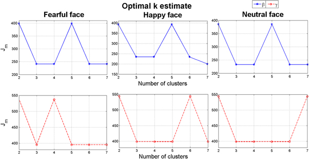
Figure 4. k-means clustering result of β and γ band for the typical group.
Download figure:
Standard image High-resolution imageIn figure 5, from the corresponding head-plots it is evident that the topographies of all three synchrostates are very similar for all the different stimuli in the β band. A similar result is observed for the γ band in figure 6 where the synchrostate topographic plots are similar and more importantly closely resemble those obtained in the β band, although differing slightly in the numerical values, in particular in the reddish hue regions. Here, each of the colours in the head topographies signify a particular range of phase differences as shown in the legend (in a normalized scale with respect to the maximum and minimum phase difference amongst all the states). However, an interesting difference is observed in the state transition plots shown in figure 7. Although in both bands the transitions start from state 2, the overall transition patterns are markedly different not only between the β and γ band but also between different stimuli within a band. This demonstrates the stimulus specific nature of the synchrostates.

Figure 5. The topographic map for all three stimuli in the β band for the typical group.
Download figure:
Standard image High-resolution image
Figure 6. The topographic map for all three stimuli in the γ band for the typical group.
Download figure:
Standard image High-resolution image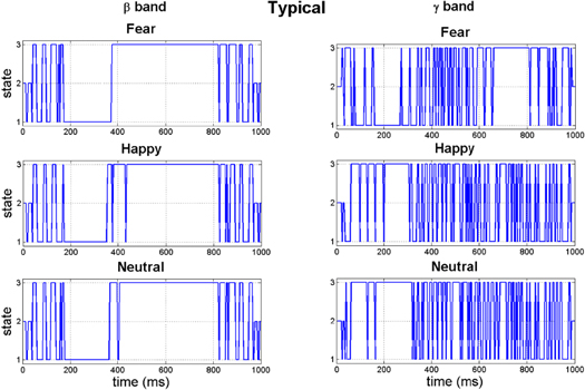
Figure 7. The time-course plot of synchrostate transitions in the β and γ band.
Download figure:
Standard image High-resolution image3.2. ASD
The k-means clustering results for the ASD population (group II in table 1) is shown in figure 8 for the β and γ bands for all three applied stimuli, i.e. fearful, happy and neutral faces. Once again the significant knee appears at k = 3 implying the existence of three synchrostates similar to the typical case. The corresponding phase difference topographies over the scalp are shown in figures 9–10 as head plots. It appears that although the stimuli are different, the topographies are nearly similar in the β bands (in figure 9) in particular for state 1 and state 3. However, topographies corresponding to state 2 are markedly different. On the other hand, in the γ band the state 1 for happy and neutral stimuli are similar, while it differs significantly for fear stimulus (figure 10). State 3 shows close similarity under all three stimuli. The time-course plots of the synchrostate transition are shown in figure 11. In both bands the time course plots are markedly different depending upon the stimulus and thereby indicating a different temporal stability period of the synchrostates at different points in time.
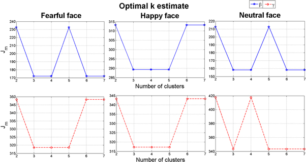
Figure 8. k-means clustering result of the β and γ band for the ASD group.
Download figure:
Standard image High-resolution image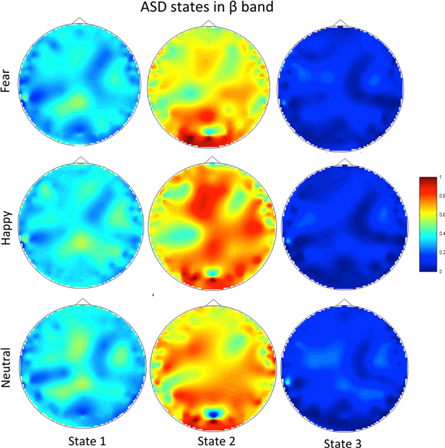
Figure 9. The topographic map all three stimuli in the β band for the ASD group.
Download figure:
Standard image High-resolution image
Figure 10. The topographic map for all three stimuli in the γ band for the ASD group.
Download figure:
Standard image High-resolution image
Figure 11. The time-course plot of synchrostate transitions in the β and γ band.
Download figure:
Standard image High-resolution image3.3. Low anxiety
The k-means clustering when run on the population average of the children with low anxiety for the β band resulted in four states for all three stimuli, i.e. angry, happy and neutral face. This is shown in figure 12 as all three plots have the earliest significant 'knee' in the cost function plot at k = 4. However, in the γ band the number of states is different for the neutral face perception case. The number of states in the γ band for the angry and happy face remain unchanged at k = 4 whereas for the neutral face it is 6. In the head topographies for the β band, (figure 13) although the number of synchrostates is consistently four, their characteristics for each different task are quite different. From the γ band head plots in figure 14 it can be seen that states 1, 4, 5 and 6 head plots are almost similar and common for all three stimuli. However the neutral stimulus has two extra states which do not exist in the other two stimuli of angry and happy, as can be seen from figure 14. The transition of the states in the β band is shown for each specific stimulus in figure 15. It can be observed that during the execution of the angry face stimulus the inter-state transition is not as frequent as compared to the other two stimuli viz. happy and neutral. The β band state transition shows that except for the angry stimulus for both the other stimuli the sequence starts with state 4, whereas for the angry visual stimulus it starts from state 2. In the γ band, the state transitions are more frequent in the neutral face perception compared to the other two stimuli, as shown in figure 15.

Figure 12. k-means clustering result of the β and γ band for the low anxiety group.
Download figure:
Standard image High-resolution image
Figure 13. The topographic map for all three stimuli in the β band for the low anxiety group.
Download figure:
Standard image High-resolution image
Figure 14. The topographic map for all three stimuli in the γ band for the low anxiety group.
Download figure:
Standard image High-resolution image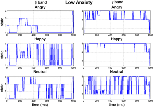
Figure 15. The time-course plot of synchrostate transitions in the β and γ band.
Download figure:
Standard image High-resolution image3.4. High anxiety
For the group of high anxiety subjects, as shown in figure 16, for both bands the number of synchrostates is consistently four for different stimuli. The head plots for the average β responses of the children as can be seen from figure 17 are to some extent similar across all the stimuli. This close similarity is even more prominent in the γ band head plots depicted in figure 18. Looking at the transitions of the states in β, shown in figure 19, we see that they end in state 1 for all three stimuli. Also state 3 is the most occurring state over the duration shown for the happy and neutral face. This is also the case for γ band state transitions for all stimuli, as shown in the figure 19.
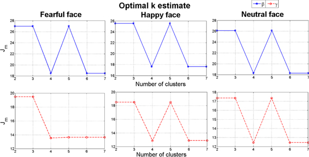
Figure 16. k-means clustering result of the β and γ band for the high anxiety group.
Download figure:
Standard image High-resolution image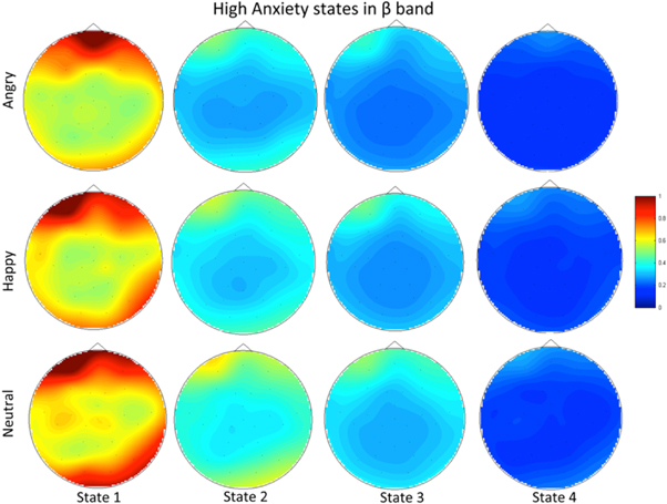
Figure 17. The topographic map for all three stimuli in the β band for the high anxiety group.
Download figure:
Standard image High-resolution image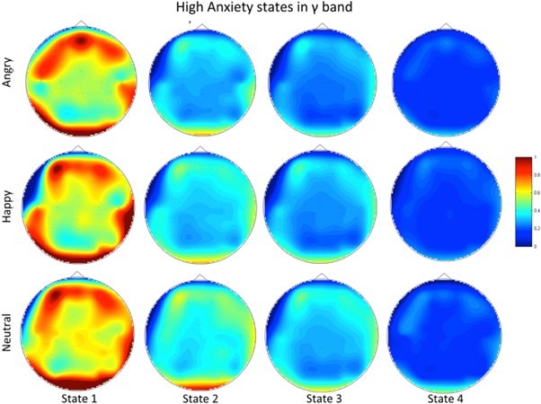
Figure 18. The topographic map for all three stimuli in the γ band for the high anxiety group.
Download figure:
Standard image High-resolution image
Figure 19. The time-course plot of synchrostate transitions in the β and γ band.
Download figure:
Standard image High-resolution image3.5. Variability analysis for individual subjects
So far the reported figures for the group-wise analysis highlight subtle changes in the average phase difference topographies over the scalp and state transition plots for different stimuli. Now the statistical measures like the median, inter-quartile ranges of the inter-person variability for the optimal number of synchrostates in both β and γ band are shown in the box-plots given in figure 20. The red line in the plot indicates the median and the crosses show the outliers. The blue boxes denote the inter quartile range for the data. This is obtained by applying k-means clustering on the phase-difference matrices obtained from individual subjects at different time instants under different stimuli. The variability in the number of synchrostates observed when results from the individual subjects are compared to the respective population average is not significant. For the pool of typical children we consistently got three states for every child in the γ band but in the β band the number of states for the children varies from 3 to 7. This observation leads us to believe that the number of synchrostates is person-specific, although this number is bounded within a small range only. Also in figure 20, for the ASD group in the β and γ band, only a few subjects show 5 synchrostates whereas the population average result as well as for the other subjects, the number of synchrostates is consistently 3. For the low anxiety and high anxiety groups (low-density EEG) it is interesting to note that the median of the number of synchrostates varies between 5 and 6 whereas the median is consistently 3 for the ASD and typical children (high-density EEG). The important factor to note here is that only 30 electrodes were used for EEG acquisition for the anxiety groups (III and IV). This reduced number of electrodes inherently introduced less resolution in computing the phase difference matrix and as a consequence may introduce a larger variability in the synchrostate formulation. Therefore it is evident that the optimal number of synchrostates largely depends on the number of electrodes and high-density EEGs (as in the first two groups, typical and ASD) are more likely to give a consistent result. Apart from that, the small variability observed in all four cases is also expected because of inter-person and inter-trial variability, and the possible existence of parallel background processes not related to the cognitive task given.

Figure 20. Box-plot of the variation in the optimal number of synchrostates in each group of subjects.
Download figure:
Standard image High-resolution image3.6. Quantification of the synchrostate transition
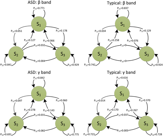
We now model the temporal switching sequence of the synchrostates in a probabilistic framework for a representative case of the typical and ASD group. This is chosen due to the fact that the high-density EEG system used in data acquisition for these two groups resulted in consistent results in synchrostates as mentioned earlier. However without loss of generality the same method could be applied for analysing the anxiety groups as well. We construct the transition probability ( of the synchrostate sequence which show the probabilistic nature of each of the state transitions. Here, nij is the number of transitions from state i to j. The three probability values—P11, P22, and P33—show how long each state remain stable, i.e. how stable each of the states (
 are in terms of the probability of staying in the same state, for different population groups, as shown in figure 21. The elements of the state transition matrix (
![${P}_{ij},\left\{i,j\right\}\in \left[1,\;2,\;3\right])$](https://content.cld.iop.org/journals/2057-1976/1/1/015002/revision1/bpex516831ieqn35.gif) for different population are more informative, although the phase difference topographies for two different populations could be similar. Therefore, the average value of the self-transitions (
for different population are more informative, although the phase difference topographies for two different populations could be similar. Therefore, the average value of the self-transitions ( N being the optimal number of synchrostates) for a particular band, can be considered as one of the discriminating measures between two groups as shown in table 2. It is evident from table 2 that in the β band with fear and happy stimuli the ASD group has got a higher probability of self-transition than the typical case. On the contrary the γ band shows an increase in self-transition for fear and neutral stimuli.
Figure 21. Average state transition (across different stimuli) diagrams for the typical and ASD group in the β and γ band.
Download figure:
Standard image High-resolution image
Table 2. Self-transitions in the β and γ band for the typical and ASD group with different stimuli.
| Typical | ASD | |||
|---|---|---|---|---|
| Stimuli | β | γ | β | γ |
| Fear | 0.843 293 | 0.756 196 | 0.880 439 | 0.880 439 |
| Happy | 0.834 324 | 0.695 356 | 0.904 088 | 0.674 856 |
| Neutral | 0.880 439 | 0.684 694 | 0.757 696 | 0.752 797 |
4. Discussion
The results shown in the foregoing section indicate that when observing in the sub-second order temporal resolution, the phase difference topography and hence phase synchronisation between EEG electrodes distributed over the scalp for all four populations is bounded within a small number (typically 3–7) of unique patterns. These results are based on the sensor or scalp level EEG synchronisation analysis. It is well known that often the scalp level synchronization with zero phase lag could be confounded by the effect of volume conduction. Therefore, a similar method for synchrony analysis could be done at the source level. Because of the lack of spatial resolution in EEG, source level synchrony gives more reliable physiological interpretations. But the very nature of source level synchrony analysis suffers from the lack of temporal resolution, restricting such methods for carrying out transient analysis of brain dynamics at fine temporal granularity level. One way to capture this effect is to translate the EEG to the corresponding source level using inverse mapping techniques. However it is well recognized that reconstructing source activity from EEG is an ill-posed problem and using EEG alone cannot uniquely determine the spatial locations of the underlying sources. Theoretically, only an infinite number of electrodes on the scalp would allow the unique determination of the locations of the sources inside (Koles 1998). Therefore, one has to make some assumptions about the inverse problem to obtain optimal and unique solutions, which leads to approximate sources (Phillips et al 2005).
4.1. Possible artifact and volume conduction effect
Before continuing discussion about the implications of this result one needs to eliminate possible artefact effects that may bias the observation. Once again we need to emphasize that the head plots shown here are fundamentally different from those obtained from qEEG analysis where the average power spectrum is plotted over the scalp. Any possible artefact in such cases is manifested as a strong correlation at the scalp edges. On the contrary, the head plots shown here are more like the visualization of the phase difference patterns distributed over the scalp. The bluish hues imply nearly zero phase difference whereas the reddish hue implies large phase difference.
Here, each of the head plots show phase difference topographies existing of the order of ms. While processing the data, as mentioned in section 2, we eliminated the epochs above 200 μV as possible artefacts. Therefore the data used in our analysis is likely to be artefact free in the first place. Secondly, since the synchrostate topographies are constructed in the ms order and as the transition diagrams show that the topographies switch from one configuration to another and back, in the ms order time interval, in the presence of possible artefacts, all of the states should exhibit a similar phase relation at the scalp edge for all the states, which is not the case. Therefore, while interpreting the results one may eliminate the effect of possible artefacts. This argument is also valid for eliminating the effect of volume conduction, which one may also view as possible artefacts. The synchrostate phenomenon we report here cannot be explained by volume conduction since electrical impulses within the human brain spread almost instantaneously through any volume. Hence, zero phase lag is a characteristic of volume conduction (Thatcher et al 2008) and phase delays are attributes of network formation. Synchrostates do not report zero phase delays and thus this suggests that the synchronies are not artefactual. In addition, the spurious synchronisation phenomena typically observed due to the presence of volume conduction does not account for the different synchronisation and desynchronisation patterns in the ms order in the switching characteristics of the synchrostates, as such an effect is expected to be present for all the synchrostate topographies in that case, while in reality the synchrostate topographies for a stimulus are different from each other. Synchrony caused due to volume conduction would render a constant synchronisation pattern (phase difference) throughout the scalp over the observed time-course of the signal. This is not the case in synchrostates as the phase patterns change suddenly both in strength and between electrodes over time and again remains stable for a finite duration. From these points one may conclude that the results shown in this work are not due to possible artefacts but manifestation of the phenomena of transient phase difference dynamics triggered by different face perception stimuli.
4.2. Existence of synchrostates
The most important finding of this study is that over the four different subject groups and a total of 44 subjects a small set of unique phase difference patterns—synchrostates—each being stable of the order of ms, have been found to exist in the β and γ band. These synchrostates switch from one to another abruptly, thereby constructing a characteristic time-course to the applied stimulus. This is qualitatively similar to the results obtained with microstates (Koenig et al 2005), albeit the microstate topographies are constructed in the EEG amplitude domain where the number of states is up to 10. From our experiments, we observe that the number of synchrostates is bounded between 3 and 7 depending on individual subjects, stimuli and also the number of EEG electrodes for recording. From the time-course plots it is evident that different synchrostates show a different duration of stability at different time points depending on the applied stimulus and thereby possibly capturing the dynamics of phase synchronisation at a finer temporal granularity level.
An interesting observation for the case of typical development population is that the topographies of population average synchrostates are almost similar for all the applied stimuli in both bands. This is similar to our earlier observation (Jamal et al 2013a, 2013b) where initial exploration was carried out with a single normal adult subject. Intuitively this implies that although different stimuli have been applied, since all of them belong to the general class of face perception task, the fundamental phase relationship over the scalp remains nearly the same, indicating a specific type of information integration phenomenon pertaining to the general face perception scenario. However the effect of different stimuli within the general class of face perception is reflected in the respective time-course plot which showed a marked difference as the characteristic of the applied stimulus. On the other hand, although the topographies in the case of ASD population showed certain similarities, they are more variable compared to the typical case along with their time-course. This may be due to the difference in information processing in the brain between the two subject groups. In addition, it is apparent that generally for the ASD group the gross phase difference of each electrode across the scalp is higher than that compared to the typical group as there are more red and yellow hues in the ASD states in the γ band (figure 10) compared to more blue hues in the states for the typical (figure 6) group. This implies predominantly loose synchronisation in the former case, which also falls in the line of already established theory that ASD brains show less synchronisation in information processing compared to typically growing children. Individuals with autism present atypical neural activity in face processing and eye gaze tasks, and this has been associated with later diagnosed autism (Elsabbagh et al 2012). Similar considerations apply to the children with anxiety. However, as discussed in section 3.5 it seems that determination of the optimal number of synchrostates depends on the electrode systems used for EEG recording and more consistent results could be obtained using a high-density system. Given this fact a direct comparison between groups I–II and III–IV could be misleading as they do not share the same number of electrode configurations. But despite this fact it is evident that the number of synchrostates in all four cases does not vary widely and is bounded within a small number of 3–7 depending on the pathophysiological conditions of the subject.
4.3. Physical interpretation
Synchrostates are the states within which the inter-electrode relative phase difference varies little over time, and the corresponding transition plot indicates how long each of these phase-difference topographies remain stable. Hence the interpretation of these states cannot be done in an isolated way from its transition plots. Interpretation of the synchrostate topographies and the state transitions should be done together, combining the stability duration and their respective numerical values of phase difference. When considered together one can formulate a synchronisation index corresponding to each of the synchrostates from which a scalp-level functional connectivity network could be derived. These dynamic networks are governed by the nature of switching patterns of the synchrostates and therefore in essence capture the temporal evolution of functional connectivity in a stimulus-specific way at fine temporal granularity level. Fundamental graph-theoretic measures could be used for characterizing such networks for gaining quantitatively deeper insight into the temporal dynamics of the connectivity pattern prevailing after the onset of stimuli, and therefore may provide a quantitative means for assessing cognitive functionalities. This approach has been adopted in (Jamal et al 2014) to classify a population of typical and ASD children. Therefore, synchrostates and their associated temporal switching sequences may be considered as a new tool for analysing the scalp-level functional connectivity dynamics at a fine temporal scale, given a type of stimulus indicating towards the dynamics of information exchange in a person-centric, and frequency band-specific manner. A major implication is that comparing the graph-theoretic measures, extracted from the functional connectivity networks formulated through synchrostates, may provide a new way of classifying different neurodevelopment disorders.
Why such synchrostates exist and, given the fact that EEG has poor spatial resolution, how the phase difference configurations described by the synchrostates corroborate with the actual anatomical level (or source level) connectivity and information exchange, is still an open question and requires further experiments and modelling activities. Thus the neurological perspective of synchrostate topographies, their numbers and transitions needs to be explored in future research. Another important fact is that the results reported here are only for face perception tasks. Whether the same phenomenon exists with other types of stimuli, e.g. auditory stimuli or different real-life cognitive activities is still a question to answer. Also whether the existence of synchrostates is associated only with the active cognitive states or not, is an area to explore.
5. Conclusions
Our analysis described in this paper shows that there exist a small set of unique phase difference patterns at ms order time intervals amongst the EEG electrodes when 44 subjects from three different neuro-pathological groups and one healthy group were subjected to a set of facial perception tasks. These unique patterns—termed as synchrostates—abruptly switch from one to another and construct a stimulus-specific time course. The synchrostates and their transition plots can together be utilized as a generic method to understand the temporal dynamics of EEG phase synchronisation as was done in (Jamal et al 2014). Our present exploration shows that the existence of such synchrostates is consistent and exhibits only a small variability that may be attributable to the inter-person or inter-trial variation often expected to be present in such experiments. Another possible factor that may contribute in such variability is the number of electrodes—fewer EEG electrodes exhibiting greater variability by introducing less resolution in computing the phase difference pattern. Also, quantification of the synchrostate transition in different groups is done in a probabilistic frame in terms of the self-transitions, which might help in understanding the EEG phase synchronisation-based derivation of the functional brain connectivity. Although we observed a consistent number of synchrostates, their physiological origin in relation to the anatomical brain network is yet to be established. Also it is still an open question whether the existence of synchrostates is a general phenomenon associated with active cognitive computation. However, if established as a generic phenomenon, combining the phase topographies of the synchrostates and their temporal stability from the time-course plot, one may establish a set of quantitative indices that may give a deeper understanding of the transient phase relationship with effective connectivity in the brain, which may be useful in quantifying cognitive ability in a task-specific manner as well as classifying atypical neuropsychiatric conditions from normal brain functionality.
Acknowledgments
The work presented in this paper was supported by the FP7 EU funded MICHELANGELO project, grant agreement # 288241. URL: www.michelangelo-project.eu/.