Modeling coherent errors in quantum error correction

Progress in fault-tolerant quantum computation relies on the ability to simulate the performance of quantum error correcting codes. For example, the numerical prediction of a high fault-tolerant error threshold for the surface code [1] is one of the motivating factors in the significant recent experimental effort to realize topological codes [2–4]. Numerical predictions of performance metrics such as the fault tolerant threshold and the logical failure rate typically assume a stochastic (incoherent) and uncorrelated Pauli channel model for physical qubit errors, since this model is easiest to simulate. However, recent findings indicate that a Pauli channel significantly underestimates the diamond norm error rate of coherent errors—errors that are both unitary and slowly varying relative to the gate time [5–8]. Such errors can occur, for example, due to systematic control noise, cross-talk, global external fields, and unwanted qubit–qubit interactions. It is therefore important to examine the accuracy of the Pauli approximation for coherent errors in the context of quantum error correction (QEC).

A variety of results have recently appeared that evaluate the impact of realistic noise on QEC. The numerical work of [9–11] has lent support to using a Pauli model for certain types of incoherent errors. These authors performed simulations of QEC for amplitude and phase damping and the corresponding Pauli-twirl approximations, finding no significant difference in logical error rates. This is consistent with a recent result of Wallman which states that non-unital deviations from Pauli channels (as in amplitude damping) do not significantly impact the error rate [7].

A different result was obtained by Fern et al [12] in the case of coherent errors. Using a formalism developed by Rahn et al [13] for general noise, these authors found that coherent errors in the physical error channel can lead to coherent errors in the logical channel, as manifested by off-diagonal elements in the superoperators for these channels. For the specific example of the d = 3 Steane code, [12] found that an off-diagonal element of order in the unencoded error superoperator leads to an encoded (logical) error superoperator with off-diagonals of order ${\epsilon }^{3}$ and diagonals of order ${\epsilon }^{4}$. This leads to a diamond-distance logical error rate of order $1/\epsilon$ greater than would be obtained by replacing the physical error by its Pauli twirl. The same result was also obtained numerically recently [14].

Another recent paper has reported diamond-distance logical error rates for surface codes up to distance d = 10 for coherent physical errors [15]. That work also finds discrepancies between coherent physical errors and their Pauli twirl approximation that are consistent with coherent errors at the logical level.

Despite these insights, it remains a challenge to obtain analytic expressions for the logical error map for general noise as a function of arbitrary code distance and (for concatenated codes) concatenation (i.e., for arbitrarily large codes). Such information can be useful for determining parameter regimes where a Pauli model is valid, and for providing independent validation of numerical results. Indeed, [12] considered general channels, deriving upper bounds on superoperator coefficients for the logical error, but not their actual value except for the d = 3 Steane code. The results of [13] were limited to diagonal channels, while [14, 15] evaluated the logical noise maps numerically, a technique which does not make explicit the scaling of the logical error parameters with d. The latter references also considered coherent and incoherent errors individually but not simultaneously.

Our aim in the present work is to obtain analytic expressions for the logical error map due to a combination of coherent and incoherent physical noise, since both are present in real qubits. We work with the repetition code, which, though not a full quantum code in that it cannot correct both X and Z errors, has the advantage of being analytically tractable and yet nontrivial. Indeed, we find that it reproduces the key features of generic codes, saturating the bounds on error channel parameters under concatenation given in [12].

Our analysis is restricted to the case of a quantum memory (or of gate-independent errors) and perfect syndrome extraction. Consideration of gate-dependent and syndrome extraction errors is left for future work. We also do not consider coherent leakage errors [6, 16] or coherent errors due to residual qubit–qubit interactions.

We derive an analytic expression for the logical error channel for arbitrary code distance d and concatenation level n, in the small error limit. (By small error limit we mean that the error rate is much less than one, irrespective of the threshold. In practice, our results apply to error rates below threshold. We give more precise definitions below.) We use a decoder optimized for independent Pauli errors—i.e., a decoder that selects the minimum-weight Pauli error consistent with the syndrome and associates a corresponding Pauli recovery operator. We find that the coherent contribution to the logical error—as quantified by the infidelity of the entire quantum computation—becomes important only after a timescale (number of QEC cycles) ${\tau }_{\mathrm{coh}}$ that increases exponentially with the size of the code. (See equation (25) and the accompanying discussion.)

Our analysis predicts the same scaling of the failure rate with the error model parameters as one obtains using the diamond norm error metric. However it emphasizes the nature of the error process as it unfolds in time. In particular, the coherent error will not be important at modest code distances for which ${\tau }_{\mathrm{coh}}$ is longer than the correlation time of the physical error. When this is the case, replacing the physical error by its Pauli-twirl accurately determines the logical error probability for quantum computations of arbitrary length. When it is not the case, there will be a critical number of correction cycles above which the persistent coherent logical error will cause logical failure more quickly than the Pauli model would predict, and this may need to be mitigated with coherent suppression methods at the physical level or larger codes. One promising way to do this is by randomization over gate sequences, which several recent papers have shown can help to combat the coherence problem [17–22].

1.1. Repetition code

We begin with a brief review of the repetition code. For more details see, e.g., [23]. The repetition code on N qubits (code distance d = N) is defined by the encoding $| \bar{0}\rangle \,=\,| 00\ldots 0\rangle$, $| \bar{1}\rangle =| 11\ldots 1\rangle$. The logical X operator, which flips $| \bar{0}\rangle$ to $| \bar{1}\rangle$ and vice versa, is denoted $\bar{X}$ and is equal to

$$\begin{eqnarray}&&\bar{X}={X}_{1}{X}_{2}\cdots {X}_{N}.\end{eqnarray} \tag{ 1 }$$

(Tensor product signs between X's are implied; they have been omitted for notational simplicity.) Bit flips (X errors) are detected by measuring the parity of neighboring qubits, which is given by the eigenvalues $({\sigma }_{1},{\sigma }_{2},\,\cdots ,\,{\sigma }_{N-1})$ of the stabilizer operators ${S}_{1}={Z}_{1}{Z}_{2}$, ${S}_{2}={Z}_{2}{Z}_{3}$, ..., ${S}_{N-1}={Z}_{N-1}{Z}_{N}$. Stabilizer eigenvalues are±1 corresponding to even or odd parity, and the set of eigenvalues is called the syndrome. $N-1$ stabilizers are required to encode a single logical qubit.

When the syndrome is measured, the state is projected onto the subspace of the Hilbert space corresponding to that syndrome. E.g., if the syndrome is $(1,1,\,\ldots ,\,1)$ then the state after syndrome extraction is in the error-free subspace, known as the codespace. If on the other hand a faulty syndrome is detected, the error can be corrected by flipping (applying the X operator to) the faulty qubit(s), thereby returning the state to the codespace. We do not pause to discuss the procedure for syndrome measurement since we assume this is done without error. Importantly, we note that the association of a syndrome to a particular error is done in a maximum likelihood rather than deterministic sense—multiple errors can have the same syndrome (e.g., X₁ and ${X}_{2}{X}_{3}$ for the N = 3 code) and we choose the one which is most likely given the syndrome. In this way we minimize the error of the encoded (logical) bits.

1.2. Error model

For an N-qubit register, we consider the error

$$\begin{eqnarray}&&{{ \mathcal N }}^{(N)}={ \mathcal N }\otimes { \mathcal N }\,\otimes \cdots \otimes \,{ \mathcal N },\end{eqnarray} \tag{ 2 }$$

where each ${ \mathcal N }$ is a single-qubit error channel. This form of error describes many of the physically relevant noise processes affecting qubits, such as cross-talk, systematic control errors, relaxation, dephasing, and external fields. An important noise source not described by equation (2) is that due to qubit–qubit interactions.

We assume the following form for the single-qubit error acting on an arbitrary input state ρ per QEC cycle.

$$\begin{eqnarray}{ \mathcal N }[\rho ] & = & (1-q){{\rm{e}}}^{-{\rm{i}}\epsilon X/2}\rho {{\rm{e}}}^{{\rm{i}}\epsilon X/2}+{{q}{X}{\rm{e}}}^{-{\rm{i}}\epsilon X/2}\rho {{\rm{e}}}^{{\rm{i}}\epsilon X/2}X\\ & = & {{\rm{\Lambda }}}_{\epsilon }\,\circ \,{{\rm{\Lambda }}}_{q}[\rho ],\end{eqnarray} \tag{ 3 }$$

where q is the probability of a stochastic bit-flip and is the angle of a small rotation error that is constant in time. We can relate these parameters to a physical dephasing rate γ and systematic rotation at rate ω (e.g., from cross-talk or an external field) through the master equation

$$\begin{eqnarray}&&\displaystyle \frac{{\rm{d}}\rho }{{\rm{d}}{t}}=-{\rm{i}}\displaystyle \frac{\omega }{2}[X,\rho ]+\gamma (X\rho X-\rho ),\end{eqnarray} \tag{ 4 }$$

by setting $\epsilon =\omega \tau$ and $q=(1-{{\rm{e}}}^{-2\gamma \tau })/2$ for a gate time (QEC cycle time) τ [24].

Equation (3) describes the composition of a coherent process, ${{\rm{\Lambda }}}_{\epsilon }$, and an incoherent process, ${{\rm{\Lambda }}}_{q}$. The latter is an appropriate description for environmentally induced decoherence as well as for random coherent rotations, such as those due to fluctuating control noise. These are described by the average over many instances of the operator $U={{\rm{e}}}^{-{\rm{i}}\theta X/2}$ applied to the quantum state, where the angle θ fluctuates from one QEC cycle to the next. (Hence q is the infidelity of the operator U, which can be related [25] to the rms rotation angle as $q={\theta }_{\mathrm{rms}}^{2}/4$.) Therefore ${{\rm{\Lambda }}}_{q}$ and ${{\rm{\Lambda }}}_{\epsilon }$ are suitable for describing the high and low-frequency components of a stochastic X rotation error. Although this error model is somewhat restrictive in that the channels ${{\rm{\Lambda }}}_{q}$ and ${{\rm{\Lambda }}}_{\epsilon }$ commute, it captures the relevant impact of coherent errors on qubit error metrics [5, 6].

We note that in general, it is possible to have a different rotation angle ${\epsilon }_{j}$ and a different bit-flip rate q_j for each qubit. We are interested in capturing the properties of errors that have broad spatial extent such as external fields. It is therefore only important that these parameters have similar (non-zero) magnitude. Choosing them all identical as in equation (2) simplifies the calculations without sacrificing any significant generality. The sign of is also not important for this discussion, and so we choose $\epsilon \geqslant 0$ throughout.

Upon logical encoding with the repetition code and using a decoder optimized for correcting independent Pauli errors, we obtain an effective error model for the logical qubit that has the same form as equation (3) but with renormalized parameters $\bar{q}$ and $\bar{\epsilon }$. This mirrors the general transformation found in [12], and stems from the fact that unital and trace preserving physical errors lead to unital, trace preserving logical errors. Such channels can be expressed as Pauli times a unitary. Non-unital deviations from Pauli channels were found in [7] to not change the error rate significantly so we do not consider them here.

We focus on low physical error rates, $q,\epsilon \ll 1$, as modern qubits routinely operate with an average error per single-qubit gate of 10⁻³ [3] down to 10⁻⁶ [26]. In this regime, we find the following expressions for the parameters $\bar{q}$ and $\bar{\epsilon }$ of the logical qubit to leading order in the physical parameters q and .

$$\begin{eqnarray}&&\bar{\epsilon }=2\left(\displaystyle \genfrac{}{}{0em}{}{d-1}{(d-1)/2}\right){\left(\displaystyle \frac{\epsilon }{2}\right)}^{d},\end{eqnarray} \tag{ 5 }$$

$$\begin{eqnarray}&&\bar{q}=\left(\displaystyle \genfrac{}{}{0em}{}{d}{(d-1)/2}\right){\left(\displaystyle \frac{{\epsilon }^{2}}{4}+q\right)}^{(d+1)/2}.\end{eqnarray} \tag{ 6 }$$

Here d = N is the code distance. The computation is elementary but lengthy. Details are given in the appendix.

Equations (5) and (6) saturate the bounds in [12]. In terms of our parameters, these bounds are: $\bar{\epsilon }$ is at most ${ \mathcal O }({\epsilon }^{d})$ and $\bar{q}-\bar{q}{| }_{\epsilon =0}$ is at most ${ \mathcal O }({\epsilon }^{2})$. The second of these bounds is not tight when q = 0, and so cannot be used to determine the impact of $\bar{\epsilon }$ on the logical error rate.

We note that the condition of low physical error rates, $q,\epsilon \ll 1$, that was used to derive equations (5) and (6), is independent of the QEC threshold. However, for the analysis to make sense the error rate must also be below threshold. We shall see below (see figure 2) that the error rate found from equations (5) and (6) decreases with increasing code distance and/or concatenation level for small enough and q. This indicates the existence of a threshold for our error model and the consistency of the small error condition with a below-threshold regime.

2.1. Discussion of decoding protocol

The logical error parameters, equations (5) and (6), were found using the standard Pauli decoder, which selects a recovery operator corresponding to the smallest-weight Pauli error that is consistent with the measured sydrome [23]. Since the stabilizers of a repetition code of distance d concatenated n times are the same as those of a repetition code of distance dⁿ concatenated once (a fact that can be readily verified by writing out the stabilizers as defined in section 1.1) it follows that the optimal Pauli decoder for n levels of concatenation of a distance d repetition code yields equations (5) and (6) with d replaced by the total number of qubits (in this case, $N={d}^{n}$):

$$\begin{eqnarray}&&{\bar{\epsilon }}_{n}=2\left(\displaystyle \genfrac{}{}{0em}{}{{d}^{n}-1}{({d}^{n}-1)/2}\right){\left(\displaystyle \frac{\epsilon }{2}\right)}^{{d}^{n}},\end{eqnarray} \tag{ 7 }$$

$$\begin{eqnarray}&&{\bar{q}}_{n}=\left(\displaystyle \genfrac{}{}{0em}{}{{d}^{n}}{({d}^{n}-1)/2}\right){\left(\displaystyle \frac{{\epsilon }^{2}}{4}+q\right)}^{({d}^{n}+1)/2}.\end{eqnarray} \tag{ 8 }$$

For a generic concatenated code, the optimal decoding could be computed using a message passing algorithm [27]. However, for generic codes it is also possible that a hard decoder (an algorithm that computes recovery operations independently at each concatenation level) would in some cases be preferable to the optimal one, for example if the computational resources for decoding are limited [28]. The result of a hard decoder optimized for Pauli errors at each concatenation level also follows from equations (5) and (6). In this case the equations give a recursion relation for the logical error between concatenation levels n and $n+1$ (n = 0 is the physical level):

$$\begin{eqnarray}&&{\bar{\epsilon }}_{n+1}=2\left(\displaystyle \genfrac{}{}{0em}{}{d-1}{(d-1)/2}\right){\left(\displaystyle \frac{{\bar{\epsilon }}_{n}}{2}\right)}^{d},\end{eqnarray} \tag{ 9 }$$

$$\begin{eqnarray}&&{\bar{q}}_{n+1}=\left(\displaystyle \genfrac{}{}{0em}{}{d}{(d-1)/2}\right){\left(\displaystyle \frac{{\bar{\epsilon }}_{n}^{2}}{4}+{\bar{q}}_{n}\right)}^{(d+1)/2}.\end{eqnarray} \tag{ 10 }$$

The number of qubits is dⁿ for each logical qubit at level n.

We note that a fully optimal decoder for the error model equation (3) (not just optimal for Pauli errors) would include coherent rotations to compensate for the parameter in equation (3). In this paper we do not consider such a decoder, and restrict ourselves to Pauli decoders, for the following reasons. (1) We do not assume the parameters q and are known. If they were, it is possible the physical qubits could be tuned in advance to the minimum level of allowed by hardware. Assuming such a tuning has been done, it would not be possible to implement the coherent parts of recovery operations intended to reduce further, as this would require a finer level of tunability than available. (2) A decoder compensating for coherent errors directly would give results that are highly specific to our particular choice of code, which would make the analysis less general.

2.2. Coherent errors and code concatenation

We now compare the dependence of coherence and logical error rates on code concatenation for the optimal Pauli decoder, equations (7) and (8) and the hard Pauli decoder, equations (9) and (10). As discussed in [6], a convenient metric for quantifying the coherence of the error is the ratio D/r of the diamond distance D [29] to the average infidelity r [25, 30] of the channel. For the error channel, equation (3), these quantities are [6]

$$\begin{eqnarray}&&r=\displaystyle \frac{2}{3}[q\cos (\epsilon )+{\sin }^{2}(\epsilon /2)],\end{eqnarray} \tag{ 11 }$$

$$\begin{eqnarray}&&D=\sqrt{\displaystyle \frac{3}{2}r-q(1-q)}.\end{eqnarray} \tag{ 12 }$$

For the purely incoherent case, $\epsilon =0$, we have $D=q=\tfrac{3}{2}r$. Therefore the ratio D/r should tend to 3/2 from above as the coherent contribution becomes negligible.

We define a coherence metric,

$$\begin{eqnarray}&&c={\mathrm{log}}_{10}\,\left(\displaystyle \frac{2D}{3r}\right),\end{eqnarray} \tag{ 13 }$$

which is 0 when the channel is incoherent and increases with increasing coherence in the channel. In figure 1 we plot the coherence metric c for d = 3, $n=0,1,2$ and a broad range of initial values of $\epsilon ,q\ll 1$. (For illustration, we choose a range that is well beyond the capabilities of present-day qubits.) At the physical level (n = 0) and first logical concatenation level (n = 1), both the optimal and hard decoders give the same results. For the hard decoder, the lower left panel of figure 1 shows that the error is effectively incoherent (c = 0) in the entire range of and q for n = 2. For the optimal decoder, d = 3, n = 2 is equivalent to d = 9, n = 1, and the lower right panel of figure 1 shows that the logical error contains some level of coherence at n = 2 for a range of and q.

Zoom In Zoom Out Reset image size

These results can be understood as follows. In the limit of low error rate that we are interested in ($\epsilon ,q\ll 1$) we have that ${\bar{q}}_{n},{\bar{\epsilon }}_{n}\ll 1$ in equations (7) and (8) or equations (9) and (10) for any n. Equations (11) and (12) then give

$$\begin{eqnarray}&&\displaystyle \frac{{\bar{D}}_{n}}{{\bar{r}}_{n}}\approx \displaystyle \frac{3}{2}\displaystyle \frac{\sqrt{{\bar{q}}_{n}^{2}+{\bar{\epsilon }}_{n}^{2}/4}}{{\bar{q}}_{n}+{\bar{\epsilon }}_{n}^{2}/4}.\end{eqnarray} \tag{ 14 }$$

Therefore the error channel is incoherent if ${\bar{\epsilon }}_{n}\ll {\bar{q}}_{n}$. For the hard decoder, equations (9) and (10) show that this occurs when both $n\geqslant 2$ and $d\geqslant 3$ for any initial $q,\epsilon \ll 1$. Hence only two levels of concatenation are necessary to obtain a logical error channel that is effectively stochastic (i.e., c = 0), for any size repetition code. For the optimal decoder on the other hand, taking the ratio of ${\bar{\epsilon }}_{n}$ and ${\bar{q}}_{n}$ in equations (7) and (8) shows that ${\bar{\epsilon }}_{n}\ll {\bar{q}}_{n}$ can fail to hold when $\epsilon \gtrapprox q$. The region where the N = 9 logical error has non-negligible coherence (lower-right panel in figure 1) satisfies this inequality. When $\epsilon \gg q$, for example, we have ${\bar{\epsilon }}_{n}/{\bar{q}}_{n}\sim 1/\epsilon$, which is much greater than one for $\epsilon \ll 1$.

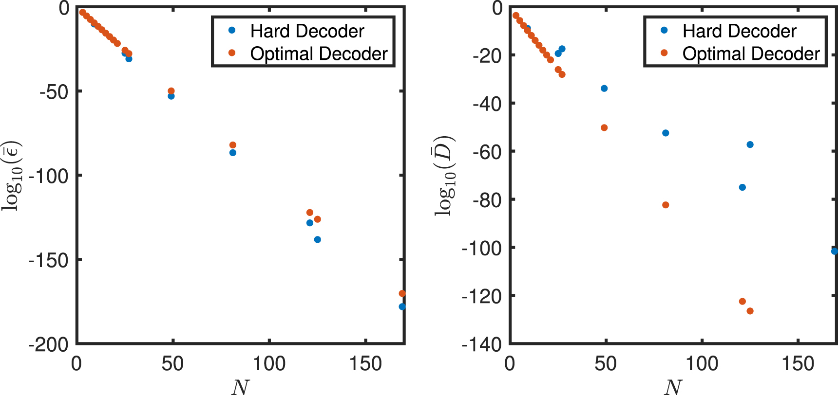
It would therefore appear that the hard decoder is better at mitigating coherent errors than the optimal decoder. Figure 2 sheds additional light on the matter. Here the logical rotation angle $\bar{\epsilon }$ and the diamond norm logical error rate $\bar{D}$ for both decoders are plotted versus the total number of qubits $N={d}^{n}$ for a range of distance d and concatenation level n. The values shown are for a single choice of physical parameters, $\epsilon =0.1$ and q = 0. This choice was made because both $\bar{\epsilon }$ and $\bar{D}$ are largest when q = 0 for a given total physical error rate $r\approx 2(q+{\epsilon }^{2}/4)/3$. Also, it satisfies our requirement that $\epsilon \ll 1$ and gives a total physical error rate that is below threshold, as can be seen in Figure 2, where the logical error rate decreases with code size.

Zoom In Zoom Out Reset image size

Both decoders show a similar suppression of $\bar{\epsilon }$ with N. Indeed, equations (7) and (9) show that ${\bar{\epsilon }}_{n}\propto {\epsilon }^{{d}^{n}}$ for both decoders. However, the optimal decoder suppresses the logical error rate $\bar{D}$ much more rapidly with N than the hard decoder. The reason is that the optimal decoder is more effective at suppressing incoherent errors, as may be expected from a decoder optimized for Pauli errors.

Hence, while the hard decoder practically eliminates the relative coherence of the error for $n\geqslant 2$, the optimal decoder provides a better logical error rate for a given number of qubits N. This illustrates the types of performance tradeoffs that can play a role when selecting a particular decoder and values of d and n for a given total number of qubits N.

2.3. Logical time to failure

We now examine the logical time to failure of the encoded qubit. As a failure metric we use the diamond norm and also the worst-case infidelity [7], since the latter naturally arises in a simulation of the time evolution. We show that both metrics give the same result for the failure time. The worst-case infidelity after m QEC cycles is defined as

$$\begin{eqnarray}&&w(m)\equiv \mathop{\max }\limits_{| \psi (0)\rangle }[1-\langle \psi (0)| \rho (m)| \psi (0)\rangle ].\end{eqnarray} \tag{ 15 }$$

This is the maximum probability of logical failure over all initial states. Here $\rho (m)$ is the state of the logical qubit after m QEC cycles,

$$\begin{eqnarray}&&\rho (m)=\mathop{\underbrace{\bar{{ \mathcal N }}\,\circ \,\cdots \,\circ \,\bar{{ \mathcal N }}}}\limits_{m\ \mathrm{times}}(| \psi (0)\rangle \langle \psi (0)| ).\end{eqnarray} \tag{ 16 }$$

The noise operator $\bar{{ \mathcal N }}$ is the single qubit operator, equation (3), with , q replaced by $\bar{\epsilon }$, $\bar{q}$ from equations (5) and (6). Equation (15) is satisfied for some initial state $| \psi (0)\rangle =| {\psi }^{* }(0)\rangle$. For the noise operator $\bar{{ \mathcal N }}$, $| {\psi }^{* }(0)\rangle$ is any state of the form $\cos (\theta )| 0\rangle -{\rm{i}}\sin (\theta )| 1\rangle$. This is a state whose Bloch vector is in the y–z plane and is therefore maximally affected by the X-rotation in equation (3).

Using equation (3) and the fact that ${{\rm{\Lambda }}}_{q}$ and ${{\rm{\Lambda }}}_{\epsilon }$ commute, we have

$$\begin{eqnarray}&&\mathop{\underbrace{\bar{{ \mathcal N }}\,\circ \,\cdots \,\circ \,\bar{{ \mathcal N }}}}\limits_{m\ \mathrm{times}}={({{\rm{\Lambda }}}_{\bar{q}})}^{m}\,\circ \,{({{\rm{\Lambda }}}_{\bar{\epsilon }})}^{m}\equiv {{\rm{\Lambda }}}_{\bar{q}(m)}\,\circ \,{{\rm{\Lambda }}}_{\bar{\epsilon }(m)},\end{eqnarray} \tag{ 17 }$$

where ${{\rm{\Lambda }}}^{m}$ denotes the composition of Λ with itself m times and $\bar{q}(m)$, $\bar{\epsilon }(m)$ are the effective error model parameters for m compositions of the error channel. (We use the notation $\bar{q}(1)=\bar{q}$, $\bar{\epsilon }(1)=\bar{\epsilon }$.)

Since the parameter q (or $\bar{q}$) in equation (3) can be parameterized as $q=(1-{{\rm{e}}}^{-2\gamma \tau })/2$ (see comments after equation (4)), for some time interval τ, we can write $q(m)=(1-{{\rm{e}}}^{-2\gamma m\tau })/2$. Rearranging this expression and using $\bar{q}$ instead of q we find

$$\begin{eqnarray}&&\bar{q}(m)=\displaystyle \frac{1}{2}[1-{(1-2\bar{q})}^{m}].\end{eqnarray} \tag{ 18 }$$

Since $\bar{\epsilon }(m)$ is simply the rotation angle for the composition of m rotations, each by angle $\bar{\epsilon }$, we have

$$\begin{eqnarray}&&\bar{\epsilon }(m)=m\bar{\epsilon }.\end{eqnarray} \tag{ 19 }$$

The worst-case infidelity, equation (15), of the error channel, equation (17), is

$$\begin{eqnarray}&&\bar{w}(m)=\bar{q}(m)\cos (\bar{\epsilon }(m))+{\sin }^{2}\left(\displaystyle \frac{\bar{\epsilon }(m)}{2}\right).\end{eqnarray} \tag{ 20 }$$

This formula can be derived by expressing equation (15) in terms of the Liouville representation [31] and using equations (A.33), (A.34) in the appendix for the error channel, equation (3), in this representation. We note that the worst-case infidelity is 3/2 the average infidelity, see equation (11).

Equation (20) predicts logical failure when $\bar{q}(m)\sim 1$ or $\bar{\epsilon }(m)\sim 1$. According to equations (18), (19), this occurs when $m\sim 1/\bar{q}$ or $m\sim 1/\bar{\epsilon }$, whichever gives the smaller value for m. The second condition is clear from equation (19). One way to derive the condition involving $\bar{q}$ is as follows. Assuming $m\gg 1$, the quantity ${(1-2\bar{q})}^{m}$ is well approximated by ${{\rm{e}}}^{-2m\bar{q}}$. Equation (18) then becomes $\bar{q}(m)\approx (1-{{\rm{e}}}^{-2m\bar{q}})/2$, which is ${ \mathcal O }(1)$ when the quantity $2m\bar{q}$ in the exponent is ${ \mathcal O }(1)$. Our assumption that $m\gg 1$ is therefore justified, since $\bar{q}\ll 1$ (which follows from equation (6) and our initial assumption that $\epsilon ,q\ll 1$). Denoting the number of QEC cycles to logical failure as ${m}_{\mathrm{fail}}$, we therefore have

$$\begin{eqnarray}&&{m}_{\mathrm{fail}}={ \mathcal O }(1/\max (\bar{\epsilon },\bar{q})).\end{eqnarray} \tag{ 21 }$$

The same result is found using the diamond distance as an error metric. Indeed, putting equation (11) in equation (12) gives the diamond distance after m QEC cycles as

$$\begin{eqnarray}&&\bar{D}(m)=\sqrt{\bar{q}{(m)}^{2}+(1-2\bar{q}(m)){\sin }^{2}\left(\displaystyle \frac{\bar{\epsilon }(m)}{2}\right)}.\end{eqnarray} \tag{ 22 }$$

Therefore $\bar{D}(m)\sim 1$ when either $\bar{q}(m)\sim 1$ or $\bar{\epsilon }(m)\sim 1$, as before.

Equation (20) also predicts a crossover from stochastic behavior, $\bar{w}(m)\approx m\bar{q}$, to coherent behavior, $\bar{w}(m)\approx {\sin }^{2}(m\bar{\epsilon }/2)$, above a critical number ${m}_{\mathrm{crit}}$ of QEC cycles, which satisfies ${m}_{\mathrm{crit}}\bar{q}\ll 1,\ {m}_{\mathrm{crit}}\bar{\epsilon }\ll 1$. In the limit $\bar{q},\bar{\epsilon }\ll 1/m$, equation (20) becomes

$$\begin{eqnarray}&&\bar{w}(m)\approx m\bar{q}+{\left(\displaystyle \frac{m\bar{\epsilon }}{2}\right)}^{2}.\end{eqnarray} \tag{ 23 }$$

This is a sum of two error rates, the first, $m\bar{q}$, from the incoherent channel ${{\rm{\Lambda }}}_{m\bar{q}}$ and the second, ${(m\bar{\epsilon }/2)}^{2}$, from the coherent rotation, ${{\rm{\Lambda }}}_{m\bar{\epsilon }}$. Setting these error rates equal to each other gives

$$\begin{eqnarray}&&{m}_{\mathrm{crit}}\sim \displaystyle \frac{2\bar{q}}{{\bar{\epsilon }}^{2}}.\end{eqnarray} \tag{ 24 }$$

Inserting the values of $\bar{\epsilon }$, $\bar{q}$ from equations (5) and (6) into (24) we find that the crossover from stochastic to coherent behavior of the logical error occurs at

$$\begin{eqnarray}&&{m}_{\mathrm{crit}}\sim 1/{\epsilon }^{N-1},\end{eqnarray} \tag{ 25 }$$

where $N={d}^{n}$ is the number of qubits, which holds when q = 0. In contrast, the number of QEC cycles to logical failure occurs at ${m}_{\mathrm{fail}}\sim 1/{\epsilon }^{N}$, which is ${ \mathcal O }(1/\epsilon )$ cycles greater than the crossover point. Therefore our initial assumption that $m\bar{\epsilon },m\bar{q}\ll 1$ for m below ${m}_{\mathrm{crit}}$ was valid.

It is instructive to compare these results to the stochastic error model defined by the Pauli-twirl of equations (2) and (3). This gives $\bar{\epsilon }=0$ in equation (5). The worst-case logical failure probability is then equal to the first term in equation (23), which is approximately the stochastic part of the full error probability. This model predicts a logical time to failure proportional to ${m}_{\mathrm{fail}}^{\mathrm{st}}={ \mathcal O }(1/{\epsilon }^{N+1})$. This is ${ \mathcal O }(1/\epsilon )$ longer (more QEC cycles) than when the coherent part of the error was included.

We conclude that a stochastic error model would correctly predict the logical failure rate up to ${m}_{\mathrm{crit}}$ QEC cycles, beyond which it is necessary to take account of the coherence of the error. If the correlation time of the coherent error is less than ${\tau }_{\mathrm{coh}}={m}_{\mathrm{crit}}{\tau }_{{\rm{QEC}}}$, where ${\tau }_{{\rm{QEC}}}$ is the duration of a QEC cycle, then the logical error is effectively stochastic and can be obtained by replacing the physical error, equation (3), by its Pauli twirl.

Figure 3 plots the worst-case failure probability vs number of QEC cycles for physical error parameters $\epsilon =0.1$, q = 0 and for $N=d=3$. The blue curve is the result of a Monte Carlo simulation of three data qubits initialized to $| {\psi }^{* }(0)\rangle =| 0\rangle$, each subject to the error operator, equation (3), once per QEC cycle. This is compared to the theoretical curve, equation (20), as well as the coherent and incoherent parts of equation (23). The simulation results show good agreement with equation (20). The crossover from stochastic to coherent behavior occurs at ${m}_{\mathrm{crit}}\sim 1/{\epsilon }^{2}=100$, consistent with the discussion above.

Zoom In Zoom Out Reset image size

Implementing QEC for coherent errors will be an important challenge for realizing scalable fault-tolerant quantum computing. It is now understood that despite the projective nature of QEC stabilizer measurements, coherent physical errors give rise to a logical error that is also coherent to some extent [12, 14, 15]. Several strategies for mitigating coherent errors have been proposed, including averaging over random gate sequences [17–22], and optimization of the decoding algorithm [28]. Our goal in this paper was to investigate another possibility, namely whether there exist parameter regimes in standard stabilizer QEC for which the logical error is Pauli even when the physical error is coherent. This would enable the use of existing techniques for correcting Pauli errors, and justify numerical simulations of QEC based on a Pauli error model.

To this end, we analyzed repetition code QEC for an error model containing coherent and incoherent errors. Focusing on the repetition code allowed us to obtain quantitative analytic results on the scaling of coherent and incoherent logical error rates with code distance d and concatenation level n.

We found that coherent physical errors result in logical errors that are partially coherent and therefore non-Pauli, in agreement with recent numerical studies [14, 15], but that the degree of coherence depends on the code distance and concatenation level. An analysis of the time to logical failure, based on a decoder optimized for independent Pauli errors, showed that the coherent part of the logical error is not important at fewer than ${\epsilon }^{-(N-1)}$ error correction cycles, where $\epsilon \ll 1$ is the rotation angle error per cycle for a single physical qubit and $N={d}^{n}$ is the total number of qubits. Logical failure occurs at ${ \mathcal O }(1/{\epsilon }^{N})$ QEC cycles, which is ${ \mathcal O }(1/\epsilon )$ faster than predicted by the Pauli-twirl approximation of the error. Furthermore, with a hard Pauli decoder the coherent part of the logical error is not important at any number of error correction cycles for two or more concatenation levels and small initial error rates. However, this needs to be traded against the larger total logical error which results from hard decoding as compared with optimal decoding.

Our findings lend support to using stochastic Pauli error models in the presence of low-frequency coherent errors under conditions of large enough code distance or concatenation. However, several questions remain to be addressed to justify the use of Pauli models for general coherent errors. Our error model was limited to a tensor product of single-qubit errors on data qubits only. Future work must include syndrome qubit and measurement errors, coherent leakage errors [6, 16], and gate dependence. In addition, unwanted couplings between qubits cause coherent errors that need to be included in the analysis.

Finally, while the calculations presented here are suggestive, the real test lies in their applicability to the particular QEC codes that will be implemented in real devices. To this end, we hope these results may inform further studies of, e.g., the surface code, which at present can only be done numerically. Recently, the work of Bravyi et al [32] has evaluated the impact of coherent errors on the logical error rate of quantum memory in large surface codes.

We are grateful to Marcus P da Silva for valuable discussions and to anonymous referees for their helpful comments. This document does not contain technology or technical data controlled under either US International Traffic in Arms Regulations or the US Export Administration Regulations.

We derive the logical error parameters equations (5) and (6), for the repetition code under the error model, equations (2) and (3), and a decoder optimized for independent Pauli errors. Throughout this section we will use a bold font to indicate a channel that acts in complex conjugate on the right and left of the density matrix, for example:

$$\begin{eqnarray}&&{\bf{A}}[\rho ]\equiv A\rho {A}^{\dagger }.\end{eqnarray} \tag{ A.1 }$$

Following the notation of Rahn et al [13], the effective logical error map is the composition of encoding, noise, and decoding,

$$\begin{eqnarray}&&{ \mathcal G }={ \mathcal D }\,\circ \,{ \mathcal N }\,\circ \,{ \mathcal E }.\end{eqnarray} \tag{ A.2 }$$

The encoding map for the repetition code is

$$\begin{eqnarray}&&{ \mathcal E }\,:| 0\rangle \mapsto | \bar{0}\rangle =| 00\cdots 0\rangle ,| 1\rangle \mapsto | \bar{1}\rangle =| 11\cdots 1\rangle .\end{eqnarray} \tag{ A.3 }$$

The decoding map includes syndrome measurement and recovery, followed by the inverse of encoding. It can be expressed as a sum over all syndromes,

$$\begin{eqnarray}&&{ \mathcal D }=\displaystyle \sum _{\sigma }{{ \mathcal E }}^{\dagger }\,\circ \,{{ \mathcal R }}_{\sigma }\,\circ \,{{\boldsymbol{ \mathcal Q }}}_{\sigma },\end{eqnarray} \tag{ A.4 }$$

where

$$\begin{eqnarray}&&{{\boldsymbol{ \mathcal Q }}}_{\sigma }[\rho ]=\left(\displaystyle \prod _{i}\displaystyle \frac{1+{\sigma }_{i}{S}_{i}}{2}\right)\rho \left(\displaystyle \prod _{i}\displaystyle \frac{1+{\sigma }_{i}{S}_{i}}{2}\right)={{ \mathcal P }}_{\sigma }\rho {{ \mathcal P }}_{\sigma }\end{eqnarray} \tag{ A.5 }$$

projects the state onto the space corresponding to the syndrome $\sigma =({\sigma }_{1},\,\cdots ,\,{\sigma }_{N-1})$, ${S}_{i}={Z}_{i}{Z}_{i+1}$ is the ith stabilizer, and ${{ \mathcal R }}_{\sigma }$ is the recovery operation that maps the logical state back to the codespace.

To simplify the notation, we work directly in terms of the physical qubit density matrix $\bar{\rho }$, which is initialized by the encoding, ${\bar{\rho }}_{0}={ \mathcal E }({\rho }_{0})$. The logical error map is then given by ${ \mathcal G }={{ \mathcal E }}^{\dagger }\,\circ \,\bar{{ \mathcal G }}\,\circ \,{ \mathcal E }$, where

$$\begin{eqnarray}&&\bar{{ \mathcal G }}=\displaystyle \sum _{\sigma }{{ \mathcal R }}_{\sigma }\,\circ \,{{\boldsymbol{ \mathcal Q }}}_{\sigma }\,\circ \,{{ \mathcal N }}^{(N)}.\end{eqnarray} \tag{ A.6 }$$

Defined in this way, ${\bar{\rho }}_{0}$ is a state in the codespace, ${\bar{\rho }}_{0}={{ \mathcal P }}_{0\ldots 0}{\bar{\rho }}_{0}{{ \mathcal P }}_{0\ldots 0}$, and we restrict the map $\bar{{ \mathcal G }}$ to act only on such states.

We begin by factoring the stochastic and coherent parts of the channel ${{ \mathcal N }}^{(N)}$:

$$\begin{eqnarray}&&{{ \mathcal N }}^{(N)}={{\rm{\Lambda }}}_{q}^{\otimes N}\,\circ \,{{\rm{\Lambda }}}_{\epsilon }^{\otimes N},\end{eqnarray} \tag{ A.7 }$$

where the tensor product over all qubits ${{\rm{\Lambda }}}^{\otimes N}\equiv {\rm{\Lambda }}\,\otimes \,...\,\otimes \,{\rm{\Lambda }}$ denotes the application of Λ to each qubit. The incoherent part can be written

$$\begin{eqnarray}{{\rm{\Lambda }}}_{q}^{\otimes N} & = & \displaystyle \sum _{k=0}^{N}{q}^{k}{(1-q)}^{N-k}{{ \mathcal O }}_{k}\\ & = & \displaystyle \sum _{k=0}^{(N-1)/2}{{ \mathcal O }}_{k}\,\circ \,[{q}^{k}{(1-q)}^{N-k}{\bf{I}}+{q}^{N-k}{(1-q)}^{k}\bar{{\bf{X}}}].\end{eqnarray} \tag{ A.8 }$$

Here ${{ \mathcal O }}_{k}$ is the sum over all weight-k products of ${{\bf{X}}}_{i}$'s:

$$\begin{eqnarray}&&{{ \mathcal O }}_{k}={{\bf{X}}}_{1}\otimes {{\bf{X}}}_{2}\cdots \otimes \,{{\bf{X}}}_{k}+{{\bf{X}}}_{1}\otimes {{\bf{X}}}_{2}\cdots \otimes \,{{\bf{X}}}_{k-1}\otimes {{\bf{X}}}_{k+1}+\cdots .\end{eqnarray} \tag{ A.9 }$$

where we have defined ${{\bf{X}}}_{i}[\bar{\rho }]={X}_{i}\bar{\rho }{X}_{i}$ as in equation (A.1). The channel ${{ \mathcal O }}_{N}=\bar{{\bf{X}}}$ is the lowest-weight undetectable error, and is also the logical bit-flip channel [23]. The second line of equation (A.8) comes from the identity ${{ \mathcal O }}_{j}=\bar{{\bf{X}}}{{ \mathcal O }}_{N-j}$.

We note that, since ${\bar{\rho }}_{0}$ is restricted to a stabilizer eigenspace (it is in the codespace, as noted above), ${{\rm{\Lambda }}}_{q}^{\otimes N}[{\bar{\rho }}_{0}]$ does not have matrix elements between states of different syndromes. We can write this compactly as

$$\begin{eqnarray}&&{{\rm{\Lambda }}}_{q}^{\otimes N}[{\bar{\rho }}_{0}]=\displaystyle \sum _{\sigma }{{\boldsymbol{ \mathcal Q }}}_{\sigma }\,\circ \,{{\rm{\Lambda }}}_{q}^{\otimes N}[{\bar{\rho }}_{0}]=\displaystyle \sum _{\sigma }{{ \mathcal P }}_{\sigma }{{\rm{\Lambda }}}_{q}^{\otimes N}[{\bar{\rho }}_{0}]{{ \mathcal P }}_{\sigma }.\end{eqnarray} \tag{ A.10 }$$

Continuing, we can write the coherent part of equation (A.7) as

$$\begin{eqnarray}{{\rm{\Lambda }}}_{\epsilon }^{\otimes N}[\bar{\rho }] & = & \left(\underset{j=1}{\overset{N}{\bigotimes }}{{\rm{e}}}^{-{\rm{i}}\epsilon {X}_{j}/2}\right)\bar{\rho }\left(\underset{k=1}{\overset{N}{\bigotimes }}{{\rm{e}}}^{{\rm{i}}\epsilon {X}_{k}/2}\right)\\ & = & \underset{j=1}{\overset{N}{\bigotimes }}(c-{{\rm{i}}{s}{X}}_{j})\bar{\rho }\underset{k=1}{\overset{N}{\bigotimes }}(c+{{\rm{i}}{s}{X}}_{k}),\end{eqnarray} \tag{ A.11 }$$

where

$$\begin{eqnarray}&&c\equiv \cos \left(\displaystyle \frac{\epsilon }{2}\right),\end{eqnarray} \tag{ A.12 }$$

$$\begin{eqnarray}&&s\equiv \sin \left(\displaystyle \frac{\epsilon }{2}\right).\end{eqnarray} \tag{ A.13 }$$

If $\bar{\rho }$ does not have matrix elements between states of different syndromes, as will be the case if $\bar{\rho }={{\rm{\Lambda }}}_{q}^{\otimes N}[{\bar{\rho }}_{0}]$ per equation (A.10), we find upon expanding equation (A.11) and projecting out a single syndrome σ that

$$\begin{eqnarray}&&{{\boldsymbol{ \mathcal Q }}}_{\sigma }\,\circ \,{{\rm{\Lambda }}}_{\epsilon }^{\otimes N}[\bar{\rho }]={{\boldsymbol{ \mathcal Q }}}_{\sigma }\,\circ \,\displaystyle \sum _{j=0}^{(N-1)/2}{P}_{j}{\bar{{\bf{U}}}}_{j}\,\circ \,{{ \mathcal O }}_{j}[\bar{\rho }],\end{eqnarray} \tag{ A.14 }$$

where we have defined

$$\begin{eqnarray}&&{P}_{j}={c}^{2(N-j)}{s}^{2j}+{c}^{2j}{s}^{2(N-j)}\end{eqnarray} \tag{ A.15 }$$

and

$$\begin{eqnarray}&&{\bar{U}}_{j}\equiv \displaystyle \frac{{c}^{N-j}{(-{\rm{i}}{s})}^{j}+{c}^{j}{(-{\rm{i}}{s})}^{N-j}\bar{X}}{\sqrt{{c}^{2(N-j)}{s}^{2j}+{c}^{2j}{s}^{2(N-j)}}}\equiv \exp \left(-{\rm{i}}\displaystyle \frac{{\epsilon }_{j}}{2}\bar{X}\right).\end{eqnarray} \tag{ A.16 }$$

The rotation angle ${\epsilon }_{j}$ is given by

$$\begin{eqnarray}&&\tan \left(\displaystyle \frac{{\epsilon }_{j}}{2}\right)={(-1)}^{\tfrac{N-1}{2}+j}{\tan }^{N-2j}\left(\displaystyle \frac{\epsilon }{2}\right).\end{eqnarray} \tag{ A.17 }$$

Combining now the coherent, equation (A.14), and incoherent, equation (A.8), part of the error channel, and using equation (A.7) we obtain

$$\begin{eqnarray}{{\boldsymbol{ \mathcal Q }}}_{\sigma }\,\circ \,{{ \mathcal N }}^{(N)}[\bar{{\rho }_{0}}] & = & {{\boldsymbol{ \mathcal Q }}}_{\sigma }\,\circ \,\displaystyle \sum _{j=0}^{(N-1)/2}{P}_{j}{\bar{{\bf{U}}}}_{j}\,\circ \,{{ \mathcal O }}_{j}[{{\rm{\Lambda }}}_{q}^{\otimes N}[{\bar{\rho }}_{0}]]\\ & = & {{\boldsymbol{ \mathcal Q }}}_{\sigma }\,\circ \,\displaystyle \sum _{j,k=0}^{(N-1)/2}{P}_{j}[{q}^{k}{(1-q)}^{N-k}{\bf{I}}+{q}^{N-k}{(1-q)}^{k}\bar{{\bf{X}}}]\,\circ \,{\bar{{\bf{U}}}}_{j}\,\circ \,{{ \mathcal O }}_{j}\,\circ \,{{ \mathcal O }}_{k}[{\bar{\rho }}_{0}].\end{eqnarray} \tag{ A.18 }$$

Since each term in the product ${{ \mathcal O }}_{j}\,\circ \,{{ \mathcal O }}_{k}$ is a product of ${{\bf{X}}}_{i}$'s, it follows that

$$\begin{eqnarray}&&{{ \mathcal O }}_{j}\,\circ \,{{ \mathcal O }}_{k}=\displaystyle \sum _{n=0}^{\min (j,k)}{m}_{{jk}}^{n}{{ \mathcal O }}_{k+j-2n}\end{eqnarray} \tag{ A.19 }$$

for some coefficients m_jkⁿ. It is straightforward to calculate these coefficients. Consider a single term in ${{ \mathcal O }}_{k}$ and select n of the ${{\bf{X}}}_{i}$'s in this term to coincide with terms in ${{ \mathcal O }}_{j}$. The appropriate terms in ${{ \mathcal O }}_{j}$ are chosen by selecting from $(N-n)-(k-n)=N-k$ possible ${{\bf{X}}}_{i}$'s for the remaining j − n ${{\bf{X}}}_{i}$'s in ${{ \mathcal O }}_{j}$ that contribute to the RHS of equation (A.19). This gives $\left(\genfrac{}{}{0em}{}{N-k}{j-n}\right)$ terms. Next there are $\left(\genfrac{}{}{0em}{}{k}{n}\right)$ ways to pick n ${{\bf{X}}}_{i}$'s in the given term of ${{ \mathcal O }}_{k}$. Finally there are $\left(\genfrac{}{}{0em}{}{N}{k}\right)$ terms in ${{ \mathcal O }}_{k}$. Since each term on the LHS of equation (A.19) contributes to the RHS of equation (A.19) and there are $\left(\genfrac{}{}{0em}{}{N}{j+k-2n}\right)$ terms on the RHS, we obtain

$$\begin{eqnarray}&&{m}_{{jk}}^{n}=\displaystyle \left(\genfrac{}{}{0em}{}{N}{k}\right)\displaystyle \left(\genfrac{}{}{0em}{}{k}{n}\right)\displaystyle \left(\genfrac{}{}{0em}{}{N-k}{j-n}\right)/\displaystyle \left(\genfrac{}{}{0em}{}{N}{k+j-2n}\right).\end{eqnarray} \tag{ A.20 }$$

Substituting equation (A.19) into (A.18) gives

$$\begin{eqnarray}&&{{\boldsymbol{ \mathcal Q }}}_{\sigma }\,\circ \,{{ \mathcal N }}^{(N)}={{\boldsymbol{ \mathcal Q }}}_{\sigma }\,\circ \,\displaystyle \sum _{j,k=0}^{(N-1)/2}\displaystyle \sum _{n=0}^{\min (j,k)}{m}_{{jk}}^{n}{P}_{j}{\bar{{\bf{U}}}}_{j}\,\circ \,{{ \mathcal O }}_{k+j-2n}\,\circ \,[{q}^{k}{(1-q)}^{N-k}{\bf{I}}+{q}^{N-k}{(1-q)}^{k}\bar{{\bf{X}}}].\end{eqnarray} \tag{ A.21 }$$

From this result, the logical error map can be derived given the decoding algorithm. We choose a decoder optimized for independent Pauli errors, which selects a recovery operator equal to the smallest weight Pauli consistent with the syndrome.

The syndrome, and hence recovery operator, is determined entirely by the term ${{ \mathcal O }}_{k+j-2n}$ in the above equation. It is therefore straightforward write down the error map, equation (A.6), which includes projection and recovery operations. If $k+j-2n\leqslant (N-1)/2$ then the recovery operation transforms each of the $\left(\genfrac{}{}{0em}{}{N}{k+j-2n}\right)$ terms in ${{ \mathcal O }}_{k+j-2n}$ to the identity, while if $k+j-2n\gt (N-1)/2$ then the recovery operation transforms each term in ${{ \mathcal O }}_{k+j-2n}$ to $\bar{X}$. Substituting equation (A.20) for m_jkⁿ and collecting terms, we find

$$\begin{eqnarray}&&\bar{{ \mathcal G }}({\bar{\rho }}_{0})=\displaystyle \sum _{j=0}^{(N-1)/2}\displaystyle \left(\genfrac{}{}{0em}{}{N}{j}\right){P}_{j}({A}_{j}{\bar{U}}_{j}{\bar{\rho }}_{0}{\bar{U}}_{j}^{\dagger }+{Q}_{j}\bar{X}{\bar{U}}_{j}{\bar{\rho }}_{0}{\bar{U}}_{j}^{\dagger }\bar{X}),\end{eqnarray} \tag{ A.22 }$$

where

$$\begin{eqnarray}{A}_{j} & = & \displaystyle \sum _{k=0}^{(N-1)/2}\displaystyle \sum _{n}\displaystyle \left(\genfrac{}{}{0em}{}{j}{n}\right)\displaystyle \left(\genfrac{}{}{0em}{}{N-j}{k-n}\right)\left[{\rm{\Theta }}\left(j+k-2n\leqslant \displaystyle \frac{N-1}{2}\right){q}^{k}{(1-q)}^{N-k}\right.\\ & & +\left.{\rm{\Theta }}\left(j+k-2n\gt \displaystyle \frac{N-1}{2}\right){q}^{N-k}{(1-q)}^{k}\right],\end{eqnarray} \tag{ A.23 }$$

$$\begin{eqnarray}{Q}_{j} & = & \displaystyle \sum _{k=0}^{(N-1)/2}\displaystyle \sum _{n}\displaystyle \left(\genfrac{}{}{0em}{}{j}{n}\right)\displaystyle \left(\genfrac{}{}{0em}{}{N-j}{k-n}\right)\left[{\rm{\Theta }}\left(j+k-2n\leqslant \displaystyle \frac{N-1}{2}\right){q}^{N-k}{(1-q)}^{k}\right.\\ & & +\left.{\rm{\Theta }}\left(j+k-2n\gt \displaystyle \frac{N-1}{2}\right){q}^{k}{(1-q)}^{N-k}\right].\end{eqnarray} \tag{ A.24 }$$

The sum over n runs over all values for which the combinatorial coefficients are defined. Here ${\rm{\Theta }}(x)$ is a Heaviside step function which takes the value 1 when the statement x is true and 0 when it is false.

Using Vandermonde's identity,

$$\begin{eqnarray}&&\displaystyle \sum _{n}\displaystyle \left(\genfrac{}{}{0em}{}{j}{n}\right)\displaystyle \left(\genfrac{}{}{0em}{}{N-j}{k-n}\right)=\displaystyle \left(\genfrac{}{}{0em}{}{N}{k}\right),\end{eqnarray} \tag{ A.25 }$$

we find

$$\begin{eqnarray}&&{A}_{j}+{Q}_{j}=1.\end{eqnarray} \tag{ A.26 }$$

Returning now to the full error map ${ \mathcal G }={{ \mathcal E }}^{\dagger }\,\circ \,\bar{{ \mathcal G }}\,\circ \,{ \mathcal E }$ we obtain for the effective 1-qubit logical error channel

$$\begin{eqnarray}&&{ \mathcal G }=\displaystyle \sum _{j=0}^{(N-1)/2}\displaystyle \left(\genfrac{}{}{0em}{}{N}{j}\right){P}_{j}{{\rm{\Lambda }}}_{{Q}_{j}}\,\circ \,{{\rm{\Lambda }}}_{{\epsilon }_{j}},\end{eqnarray} \tag{ A.27 }$$

where

$$\begin{eqnarray}&&{{\rm{\Lambda }}}_{{Q}_{j}}(\rho )=(1-{Q}_{j})\rho +{Q}_{j}X\rho X,\end{eqnarray} \tag{ A.28 }$$

$$\begin{eqnarray}&&{{\rm{\Lambda }}}_{{\epsilon }_{j}}(\rho )={U}_{j}\rho {U}_{j}^{\dagger },\end{eqnarray} \tag{ A.29 }$$

with U_j as in equation (A.16) with X replacing $\bar{X}$.

Equations (A.27)–(A.29) show that the effective logical error is an incoherent sum of terms, each of which is the composition of a stochastic bit flip and coherent rotation.

To enable further simplification it is helpful to use the Liouville, or Pauli transfer matrix (PTM) representation of quantum channels [31]. For an N-qubit channel this is defined as

$$\begin{eqnarray}&&{R}_{{ij}}({\rm{\Lambda }})=\displaystyle \frac{1}{{2}^{N}}\mathrm{Tr}[{V}_{i}{\rm{\Lambda }}({V}_{j})],\end{eqnarray} \tag{ A.30 }$$

where V_i, ${V}_{j}\in \{I,X,Y,Z\}{}^{\otimes N}$ are basis vectors in the vector space spanned by all tensor products of N Pauli matrices (including the identity).

The PTMs are linear functions of the channels they represent. The following identities hold for arbitrary quantum channels ${{\rm{\Lambda }}}_{1}$, ${{\rm{\Lambda }}}_{2}$ and constants a, b.

$$\begin{eqnarray}&&{R}_{{ij}}({{\rm{\Lambda }}}_{1}\,\circ \,{{\rm{\Lambda }}}_{2})=\displaystyle \sum _{k}{R}_{{ik}}({{\rm{\Lambda }}}_{1}){R}_{{kj}}({{\rm{\Lambda }}}_{2}),\end{eqnarray} \tag{ A.31 }$$

$$\begin{eqnarray}&&{R}_{{ij}}(a{{\rm{\Lambda }}}_{1}+b{{\rm{\Lambda }}}_{2})={{aR}}_{{ij}}({{\rm{\Lambda }}}_{1})+{{bR}}_{{ij}}({{\rm{\Lambda }}}_{2}).\end{eqnarray} \tag{ A.32 }$$

The logical error channel, equation (A.27), is a single-qubit channel. It contains only identity and X operators, leaving the space spanned by $\{1,X\}$ invariant. By analogy to the notation in [14] for process matrices, we can therefore write R in terms of 2 × 2 blocks,

$$\begin{eqnarray}R=\left(\begin{array}{cc}1 & 0\\ 0 & \tilde{R}\end{array}\right).\end{eqnarray} \tag{ A.33 }$$

The matrices $\tilde{R}$ satisfy the same composition properties, equations (A.31) and (A.32), as the full matrix R. Using these definitions, the matrix $\tilde{R}$ for the single-qubit error channel, equation (3), evaluates to

$$\begin{eqnarray}\tilde{R}({ \mathcal N })=\tilde{R}({{\rm{\Lambda }}}_{q})\tilde{R}({{\rm{\Lambda }}}_{\epsilon })=(1-2q)\left(\begin{array}{cc}\cos \epsilon & -\sin \epsilon \\ \sin \epsilon & \cos \epsilon \end{array}\right).\end{eqnarray} \tag{ A.34 }$$

We now write equation (A.27) as

$$\begin{eqnarray}&&\tilde{R}({ \mathcal G })=\displaystyle \sum _{j=0}^{(N-1)/2}\displaystyle \left(\genfrac{}{}{0em}{}{N}{j}\right){P}_{j}\tilde{R}({{\rm{\Lambda }}}_{{Q}_{j}})\tilde{R}({{\rm{\Lambda }}}_{{\epsilon }_{j}})\end{eqnarray} \tag{ A.35 }$$

$$\begin{eqnarray}=\displaystyle \sum _{j=0}^{(N-1)/2}\displaystyle \left(\genfrac{}{}{0em}{}{N}{j}\right){P}_{j}(1-2{Q}_{j})\left(\begin{array}{cc}\cos {\epsilon }_{j} & -\sin {\epsilon }_{j}\\ \sin {\epsilon }_{j} & \cos {\epsilon }_{j}\end{array}\right).\end{eqnarray} \tag{ A.36 }$$

We are interested in the leading order terms in this equation in , q. From equation (A.15) and the identity ${\sum }_{j=0}^{(N-1)/2}\left(\genfrac{}{}{0em}{}{N}{j}\right){P}_{j}=1$, we find to lowest order in ,

$$\begin{eqnarray}{P}_{j}\approx \left\{\begin{array}{ll}1-{\displaystyle \sum }_{k=1}^{(N-1)/2}\displaystyle \left(\genfrac{}{}{0em}{}{N}{k}\right){\left(\tfrac{\epsilon }{2}\right)}^{2k}, & j=0,\\ {\left(\tfrac{\epsilon }{2}\right)}^{2j}, & j\ne 0\end{array}\right.\end{eqnarray} \tag{ A.37 }$$

and from equation (A.24) we find, to lowest order in q,

$$\begin{eqnarray}&&{Q}_{j}\approx \displaystyle \left(\genfrac{}{}{0em}{}{N-j}{\tfrac{N+1}{2}-j}\right){q}^{\tfrac{N+1}{2}-j}.\end{eqnarray} \tag{ A.38 }$$

The last equation is found by observing that the lowest order term in q comes from the 2nd term in equation (A.24) when k takes its minimal value. This happens when n = 0 and $k=(N+1)/2-j$. Finally, from equation (A.17) we find

$$\begin{eqnarray}&&{\epsilon }_{j}\approx {\left(\displaystyle \frac{{\rm{i}}}{2}\right)}^{N-2j-1}{\epsilon }^{N-2j},\end{eqnarray} \tag{ A.39 }$$

to leading order in .

We now calculate the diagonal and off-diagonal terms in equation (A.36). The diagonal terms are

$$\begin{eqnarray}&&\displaystyle \sum _{j=0}^{(N-1)/2}\displaystyle \left(\genfrac{}{}{0em}{}{N}{j}\right){P}_{j}(1-2{Q}_{j})\cos {\epsilon }_{j}\\ &&\quad =\,\left[1-\displaystyle \sum _{k=1}^{(N-1)/2}\displaystyle \left(\genfrac{}{}{0em}{}{N}{k}\right){\left(\displaystyle \frac{\epsilon }{2}\right)}^{2k}\right]\left[1-2\displaystyle \left(\genfrac{}{}{0em}{}{N}{\tfrac{N+1}{2}}\right){q}^{\tfrac{N+1}{2}-j}\right]\left[1-2{\left(\displaystyle \frac{\epsilon }{2}\right)}^{2N}\right]\\ &&\quad +\,\displaystyle \sum _{j=1}^{(N-1)/2}\displaystyle \left(\genfrac{}{}{0em}{}{N}{j}\right){\left(\displaystyle \frac{\epsilon }{2}\right)}^{2j}\left[1-2\displaystyle \left(\genfrac{}{}{0em}{}{N-j}{\tfrac{N+1}{2}-j}\right){q}^{\tfrac{N+1}{2}-j}\right]\left[1-2{\left(\displaystyle \frac{\epsilon }{2}\right)}^{2N-4j}\right].\end{eqnarray} \tag{ A.40 }$$

Expanding and keeping the lowest order terms in q and , the above equation reduces to $1-2\bar{q}$, where

$$\begin{eqnarray}&&\bar{q}=\displaystyle \left(\genfrac{}{}{0em}{}{N}{\tfrac{N+1}{2}}\right){\left(\displaystyle \frac{{\epsilon }^{2}}{4}+q\right)}^{\displaystyle \frac{N+1}{2}}.\end{eqnarray} \tag{ A.41 }$$

This proves equation (6).

Next we calculate the off-diagonals in equation (A.36).

$$\begin{eqnarray}&&\displaystyle \sum _{j=0}^{(N-1)/2}\displaystyle \left(\genfrac{}{}{0em}{}{N}{j}\right){P}_{j}(1-2{Q}_{j})\sin {\epsilon }_{j}\\ &&\quad =\,\left[1-\displaystyle \sum _{k=1}^{(N-1)/2}\displaystyle \left(\genfrac{}{}{0em}{}{N}{k}\right){\left(\displaystyle \frac{\epsilon }{2}\right)}^{2k}\right]\left[1-2\displaystyle \left(\genfrac{}{}{0em}{}{N}{\tfrac{N+1}{2}}\right){q}^{\tfrac{N+1}{2}-j}\right]\left[2{(-1)}^{\displaystyle \frac{N-1}{2}}{\left(\displaystyle \frac{\epsilon }{2}\right)}^{N}\right]\\ &&\quad +\,\displaystyle \sum _{j=1}^{(N-1)/2}\displaystyle \left(\genfrac{}{}{0em}{}{N}{j}\right){\left(\displaystyle \frac{\epsilon }{2}\right)}^{2j}\left[1-2\displaystyle \left(\genfrac{}{}{0em}{}{N-j}{\tfrac{N+1}{2}-j}\right){q}^{\tfrac{N+1}{2}-j}\right]\left[2{(-1)}^{\tfrac{N-1}{2}-j}{\left(\displaystyle \frac{\epsilon }{2}\right)}^{N-2j}\right]\\ &&\quad \approx \,2{\left(\displaystyle \frac{\epsilon }{2}\right)}^{N}\displaystyle \sum _{j=0}^{(N-1)/2}{(-1)}^{\tfrac{N-1}{2}-j}\displaystyle \left(\genfrac{}{}{0em}{}{N}{j}\right).\end{eqnarray} \tag{ A.42 }$$

The sum in the last equation is straightforward to simplify by writing the sums over even and odd j separately and using Pascal's rule. The result is

$$\begin{eqnarray}&&\bar{\epsilon }=2\displaystyle \left(\genfrac{}{}{0em}{}{N-1}{\tfrac{N-1}{2}}\right){\left(\displaystyle \frac{\epsilon }{2}\right)}^{N}.\end{eqnarray} \tag{ A.43 }$$

This proves equation (5).

At this level of approximation (linear in $\bar{q}$ and $\bar{\epsilon }$), which is accurate when $\epsilon ,q\ll 1$, we can write the reduced PTM as

$$\begin{eqnarray}\tilde{R}({ \mathcal G })=(1-2\bar{q})\left(\begin{array}{cc}\cos \bar{\epsilon } & -\sin \bar{\epsilon }\\ \sin \bar{\epsilon } & \cos \bar{\epsilon }\end{array}\right).\end{eqnarray} \tag{ A.44 }$$

This shows that ${ \mathcal G }$ has the same form as ${ \mathcal N }$ (see equation (3)) with renormalized parameters $q\to \bar{q}$, $\epsilon \to \bar{\epsilon }$.