


Abstract
3-D full waveform inversion (FWI) of seismic wavefields is routinely implemented with explicit time-stepping simulators. A clear advantage of explicit time stepping is the avoidance of solving large-scale implicit linear systems that arise with frequency domain formulations. However, FWI using explicit time stepping may require a very fine time step and (as a consequence) significant computational resources and run times. If the computational challenges of wavefield simulation can be effectively handled, an FWI scheme implemented within the frequency domain utilizing only a few frequencies, offers a cost effective alternative to FWI in the time domain. We have therefore implemented a 3-D FWI scheme for elastic wave propagation in the Fourier domain. To overcome the computational bottleneck in wavefield simulation, we have exploited an efficient Krylov iterative solver for the elastic wave equations approximated with second and fourth order finite differences. The solver does not exploit multilevel preconditioning for wavefield simulation, but is coupled efficiently to the inversion iteration workflow to reduce computational cost. The workflow is best described as a series of sequential inversion experiments, where in the case of seismic reflection acquisition geometries, the data has been laddered such that we first image highly damped data, followed by data where damping is systemically reduced. The key to our modelling approach is its ability to take advantage of solver efficiency when the elastic wavefields are damped. As the inversion experiment progresses, damping is significantly reduced, effectively simulating non-damped wavefields in the Fourier domain. While the cost of the forward simulation increases as damping is reduced, this is counterbalanced by the cost of the outer inversion iteration, which is reduced because of a better starting model obtained from the larger damped wavefield used in the previous inversion experiment. For cross-well data, it is also possible to launch a successful inversion experiment without laddering the damping constants. With this type of acquisition geometry, the solver is still quite effective using a small fixed damping constant. To avoid cycle skipping, we also employ a multiscale imaging approach, in which frequency content of the data is also laddered (with the data now including both reflection and cross-well data acquisition geometries). Thus the inversion process is launched using low frequency data to first recover the long spatial wavelength of the image. With this image as a new starting model, adding higher frequency data refines and enhances the resolution of the image. FWI using laddered frequencies with an efficient damping schemed enables reconstructing elastic attributes of the subsurface at a resolution that approaches half the smallest wavelength utilized to image the subsurface. We show the possibility of effectively carrying out such reconstructions using two to six frequencies, depending upon the application. Using the proposed FWI scheme, massively parallel computing resources are essential for reasonable execution times.
1 INTRODUCTION
In the last decade, advances in multiprocessor computer systems and algorithms have motivated the development of a 3-D seismic full waveform inversion (FWI) technique that can recover subsurface physical parameters (e.g. velocities, density or other seismic attributes), based on data fitting and iterative optimization. This technology was first suggested in the 1980s for the time domain (Tarantola 1984,1986). Because FWI in the time domain exploits explicit time stepping, waveform inversion requires very fine time steps necessary for accurately simulating broadband seismic traces, which lead to significant consumption of computational resources and long simulation times; time windowing the seismic trace may help reduce this requirement for the time step, but may also reduce the information content. The application of multiple sources and receiver sets in industrial-sized seismic surveys, along with the difficulty of an unknown source wavelet estimation, further compounds the problem (Shipp & Singh 2002; Sheen et al.2006).
The first discussion about FWI in the frequency domain was initiated by Pratt (1990). The appeal of frequency-domain FWI is its computational efficiency under applicable conditions, achieved by limiting the inversion to a few discrete frequencies (Sirgue & Pratt 2004) where the unknown source wavelet can be estimated simultaneously during the inversion process (Pratt 1999; Shin & Min 2006). These efficiencies are clearly evident in a 2-D FWI frequency-domain formulation, because factorization and solution of the linear system required for wavefield simulation are computationally practical at each frequency with multiple right-hand sides (Marfurt 1984). This system is solved efficiently for multiple sources using a direct solver, which performs one LU factorization of the matrix, followed by a forward and backward substitution per source. However, this approach is difficult to design for 3-D wave equations (acoustic and elastic), because the frequency-domain direct solver requires extensive memory for real-sized problems (Operto et al.2007). While Wang et al. (2012a) has reported progress for the 3-D Helmholtz equation applied to acoustic wavefields, the problem is significantly worse in the case of elastic wavefield simulation, because it is now nearly an order of magnitude larger in size. Nevertheless, Wang et al. (2012b) have reported some encouraging results for simulation of elastic wave fields using a direct solver approach.
While FWI can provide high-resolution quantitative images of seismic attributes, in either domain, it comes with very high computational costs, particularly in 3-D. Therefore, the most successful and cost efficient applications of FWI are 2-D (Shipp & Singh 2002; Operto et al.2004; Brenders & Pratt 2007; Shin et al.2010). The 3-D case have been considered by Sirgue et al. (2008), Ben-Hadj-Ali et al. (2008), Warner et al. (2008), Pyun et al. (2008), Plessix (2009), Guasch et al. (2012) and Wang et al. (2012). Among the existing publications on 3-D FWI, the majority employ an acoustic approximation (assuming there is no shear wave). Published studies based on 3-D elastic wave inverse modelling (Pyun et al.2008; Guasch et al.2012) are much fewer, due to its much higher computational cost, as we have already mentioned.
It should be clear that an effective 3-D FWI in the frequency domain requires a robust solver. Even with the advances made with direct solvers the appeal of iterative solvers is strong, since they require far less computational resources and memory. While existing iterative solvers are far from optimal, new approaches for algorithms (Sonneveld & van Gijzen 2008), and pre-conditioners (Erlangga & Nabben 2008) have been developed so it is now possible to efficiently solve linear systems of sizes relevant to 3-D FWI (Plessix 2009). With a robust iterative solver, the advantages of 3-D frequency-domain FWI become apparent. It has the advantage of requiring only a few frequencies in an inversion experiment (Warner et al.2008; Plessix 2009). In this paper, we will use the iterative solver proposed by Sonneveld & van Gijzen (2008) and realized for the solution of damped elastic wavefields in Laplace–Fourier domain, using a scheme proposed by Petrov & Newman (2012). We will show that the time to solution for this problem is fast enough that we can use the solver within a 3-D FWI framework. While the solver does not exploit a multilevel pre-conditioner for wavefield simulation, we have coupled it very efficiently to the inversion iteration workflow to reduce its overall computational cost.
A major difficulty of FWI is related to the ill-posed nature and non-linearity of the inverse problem, which is generally formulated as a least-squares local optimization problem. Particularly problematic is the non-linearity exhibited by the presence of local and multiple minima in the least-squares error functional (Virieux & Operto 2009). The ill-posedness of FWI mainly arises from the lack of low frequencies in the source bandwidth and the incomplete illumination of the subsurface provided by conventional seismic surveys. Consequently, the results strongly depend on the starting model. The presence of noise in the data can also have adverse effects on image quality, particularly when such data are greatly contaminated with noise in the lower frequency band, such as in marine data acquisition below frequencies of several hertz. If such noise is not an issue or can be effectively suppressed, several hierarchical multiscale strategies that proceed from low frequencies to higher frequencies can potentially mitigate the non-linearity of the inverse problem (Pratt 1990; Bunks et al.1995; Sirgue & Pratt 2004; Brossier et al.2009). Most 3-D FWI inversion methods (time or frequency) are based on gradient approaches, such as the non-linear conjugate gradient (NLCG) method (Pratt 1999; Sirgue & Pratt 2004; Ben-Hadj-Ali et al.2008). Higher order minimization schemes such as Gauss–Newton and full Newton methods (see Pratt et al.1998; Hu et al.2009) have appeal, but can be prohibitively expensive in 3-D.
There are three main approaches to waveform inversion in the frequency domain: (1) the multifrequency simultaneous inversion (Shin & Min 2006); (2) the sequential single-frequency inversion (Sirgue & Pratt 2004; Ben-Hadj-Ali et al.2008) and (3) the combination of the two approaches (Pratt 1999). In the multifrequency simultaneous inversion, all selected frequencies are inverted jointly as in the time domain. However, this approach is very expensive, because it is necessary to process not only a large number of shots but additionally a large number of frequencies, simultaneously. Moreover, to balance the contributions from the different frequency components in the data, careful data-weighting schemes must be applied (Hu et al.2009). The sequential single-frequency inversion requires less computational resources than the multifrequency simultaneous inversion. Also, the issue frequency data-weighting is irrelevant. As a rule, the low-frequency data are less non-linear with respect to the model than high-frequency data. Thus the inversion can be successfully performed proceeding from low to high frequencies (Sirgue & Pratt 2004; Ben-Hadj-Ali et al.2008; Shin & Cha 2008, 2009).
Finally, the modeller can also combine the multifrequency simultaneous inversion approach with the sequentially ordered single-frequency inversion approach, where frequencies are binned into groups. All frequencies in each group are inverted simultaneously, and all groups are inverted sequentially, commencing from low to high frequencies (Pratt 1999; Brenders & Pratt 2007). From our experience, especially with regard to computational resources, we consider a sequentially ordered single-frequency inversion as most efficient.
To better eliminate the problem of local minima and to recover the long wavelength components of the velocity model, Brown et al. (2005), Shin & Cha (2008) proposed to use the Laplace-domain waveform inversion. Later, Shin & Cha (2009) suggested the waveform inversion in the Laplace–Fourier domain. Waveform inversion in the Laplace and Laplace–Fourier domain tries to invert Laplace-transformed wavefields, which are zero- and low-frequency components of damped wavefields using several damping constants. Application of the multiscale approach now includes not only sequential increasing frequencies, but also a range of damping factors. Motivation for extending the FWI imaging process into the Laplace domain is that the objective functional is smoother and exhibits fewer local minima than the conventional frequency-domain waveform inversion (Brown et al.2005).
In this paper, we propose a sequentially ordered single frequency 3-D elastic waveform inversion scheme using the quadratic error functional in the Laplace–Fourier domain. Our algorithm sequentially inverts single complex frequency data, which consists of the ordinary frequency and Laplace damping constant, and is designed to find an elastic attribute model from a simple initial starting model. First, we review the theory of Laplace–Fourier domain elastic wavefield modelling and inversion. Following this, we describe our multiscale strategy to mitigate the non-linearity of the 3-D elastic inverse problem. This strategy involves two loops over frequencies and damping constants in the inversion algorithm. Next, we describe a massively parallel implementation of FWI algorithm for imaging 3-D elastic media. Finally, we apply the FWI algorithm to three synthetic examples of increasing complexity, with the aim of validating the algorithm for complex media reconstructions of elastic attributes. Because of the complexity and expensive computer cost of 3-D elastic FWI, we apply our scheme to modest-sized problems to investigate its performance and define an effective workflow. Results for large-scale models and data sets will be reported in subsequent studies. Through a synthetic application of several models, including cross-well and seismic reflection acquisition geometries, we demonstrate that our strategy of sequential inversion of damped wavefields can improve the quality of the inversion results and reduce the total number of inversion iterations, by exploiting laddered frequencies and damping constants. We show that it is possible to reconstruct elastic attributes of the subsurface at a resolution that approaches half the smallest wavelength utilized to image the subsurface.
2 ELASTIC WAVEFORM INVERSION THEORY
2.1 Regularized least squares
The parameters that control model smoothness are the regularization matrix, W, which consists of a FD approximation to the gradient operator (∇m), and the regularization parameter λ, which is used to control the amount of smoothness to be incorporated into the inverse model. Large values of λ will produce very smooth models, at the expense of poorer fits to the observed data. Small parameters give superior data fits, but the resulting models can be non-physical. The typical modelling strategy is to run the inversion using several values of λ and attempt to find an acceptable match to data within observational errors. Of those models that match the data, the model with the smoothest set of characteristics is selected. This model will correspond to the largest acceptable regularization parameter.
We minimize the objective functional in eq. (1) using the NLCG method (Fletcher & Reeves 1964; Polyak & Ribière 1969) following the implementations of Newman & Alumbaugh (1997, 2000) and Commer & Newman (2008). The NLCG method requires calculations of a gradient, search direction, and a step length value along the given search direction. The flowchart of our algorithm is described in detail by Newman & Alumbaugh (2000).
2.2 Computation of the gradients
2.3 Logarithmic parameters
We employ a sequential, single-frequency Laplace–Fourier-domain waveform inversion approach for imaging across multiple scales, as proposed by Tarantola (1986), Bunks et al. (1995), Pratt (1999), Sirgue & Pratt (2004) and Shin & Cha (2009). Because the frequency is now complex-valued, s = σ + iω, consisting of a Laplace damping factor σ and the angular frequency ω, waveform inversion will involve multiple real valued frequencies and damping constants. The choices made in selecting these frequencies and damping constants, and their respective ordering, is critical for a successful outcome of the inversion experiment.
Although several sequential ordering schemes for waveform inversion in the Laplace–Fourier domain have been proposed (Shin et al.2010), we favour the multiscale inversion approach, wherein frequencies are mainly changed from low to high, following the strategy suggested by Bunks et al. (1995) and Sirgue & Pratt (2004), and where the Laplace damping constant is changed from large to small values. Fig. 1(a) illustrates this waveform inversion scheme. The proposed ordering is based upon two reasons. The first reason is concerned with local minima issues that arise in FWI due to cycle skipping (Virieux & Operto 2009). To address this problem, modellers typically begin the inversion process with low frequencies and proceed sequentially to higher frequencies, employing a multiscale imaging approach (Fichtner 2011). If the inversion procedure is initiated at too high a frequency, in the absence of a very good starting model, the complexity of high-frequency wave scattering and re-radiation in heterogeneous media will produce unacceptable results. While some regions of the inversion domain may change little during the inversion iteration, other regions of the model that are illuminated will be extremely sensitive to the discontinuities of the medium. These discontinuities may be considered as secondary sources of elastic waves. So rather than rendering an accurate map of the elastic parameters, the reflectivity at interfaces is emphasized.
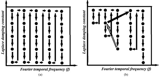
(a) The sequential downward waveform inversion in the Laplace–Fourier domain, (b) the truncated downward waveform inversion in the Laplace–Fourier domain with reverse loop.
The other reason is concerned with the efficiency of the iterative solver used for the forward problem. The convergence of the numerical solution of the system in eq. (6) strongly depends on the damping parameter σ (Petrov & Newman 2012). Our simulations show that a twofold decrease in σ, for example σ ≤ 2 s−1, leads to a doubling of the number of iterations for the same level of solution accuracy. Thus, starting the inversion process at a large damping constant at a given frequency will result in a faster overall time to solution than starting with lower damping.
However, such an order of inversion (Fig. 1a) may not be necessarily optimal, because the implementation of large damping, proceeding from lower to upper frequencies, will smooth specific structures, which were obtained with a small damping constant during the previous inversion cycle. Thus, it seems more practical not to cover the full range of damping constants at lower frequencies, but rather to truncate them to insure that image resolution will be similar to that obtained with the largest damping constant used at the next frequency. Fig. 1(b) presents the truncated cycle for the sequential waveform inversion. We will show that this strategy, when combined with multiscale imaging in frequency, can be used to great advantage to produce high-resolution 3-D images of elastic attributes in a cost-effective manner.
Additionally, we would like to note that the final solution of inverse problem must satisfy all frequencies employed in the imaging experiment independent of strategy employed. Thus, it can be very useful after inversion at high frequencies to return to the lower frequencies (Fig. 1b). This reverse loop helps preserve the content of lower frequency data in the imaging process as data with higher frequency content is added to the inversion process. Guided by general considerations that the solution must satisfy all frequencies, the return to lower frequency should be made after completion of inversion at each new higher frequency, but we believe the reverse loop can still be efficiently employed after every other laddered frequency.
3 PARALLEL IMPLEMENTATION
The FWI in 3-D for each frequency and damping constant may require several hundred iterations to obtain an acceptable solution, which can be used in the next stage of the inversion work flow. Note further the requirement of at least three forward solutions per inversion iteration. This computationally demanding problem thus needs to be implemented on a distributive computing platform with sufficient resources, which include massively parallel computing cores with large amounts of available core memory. Our inversion code uses two levels of parallelism. One of them is over the data volume (seismic sources)—that is, different source and receiver sets are assigned to different cores for the computation. Hence, the wavefields arising from multiple sources can be run in parallel on different sets of cores, independently. Another level of parallelism is over the modelling domain—spatial parallelism, or domain decomposition, which distributes the model across banks of cores. All processor communication is carried out using the Message Passing Interface (MPI) software library.
3.1 Domain decomposition
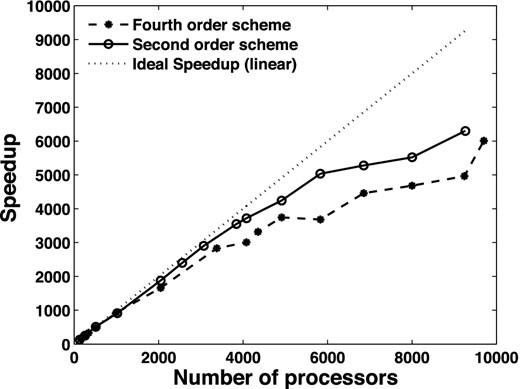
Speedup from parallel processing for a fixed-sized forward problem (588 × 588 × 261).
These results show that on the CRAT XT4 machine, our code is able to achieve a scaled speedup of 90 per cent on 4000 processors for the second-order scheme, and of 75 per cent for the fourth-order scheme. We note the decreasing efficiency of the solution beyond 4000 processors, because of the overhead due to message passing, which becomes a limiting factor in time-to-solution performance. The same parallelization scheme was applied to solve linear system (14) with Hermitian transpose matrix KH, which is required for gradient calculation.
3.2 Data decomposition
To avoid message passing overhead and subsequent inefficiencies, a second level of parallelization is realized by distributing the data such that sources and corresponding receivers of a data set are assigned to specific groups of processors. Let ndata correspond to the number of such data groups. The total number of processors or tasks employed would then be ntot = ndatanxyz. Here, ndata copies of the forward problem are distributed across the parallel machine. The data decomposition enables keeping a balance between nxyz, the size of the forward problem (dictated by the size of its corresponding FD mesh) and the number of independent source activations and frequencies. At the same time, data groups can increase linearly with the total number of sources or shots employed in the imaging experiment, given the total number of computational tasks available.
Bottlenecks for data decomposition parallelization may arise from large Krylov convergence differences between the data groups. To achieve good load balancing, the sources are distributed among the data groups such that each group has a similar workload in terms of convergence of the Krylov solver. This can be estimated in advance with a trial inversion iteration. However, it should be noted that convergence characteristics are subject to changes during later stages of an inversion, owing to changing model properties. Thus, we make the workload distribution dependent only on the seismic sources frequencies and damping constants, while nxyz is kept constant for each data group. Fig. 3 shows speedup of the fixed size FWI test problem (129 × 40 × 47 grid cells) as a function of the number of processors. The modelling was performed with the second-order FD scheme and with two variants of model decomposition (nx = 6, ny, z = 2 or nx = 3, ny, z = 1), yielding nearly identical performance. Since data decomposition is highly parallel, a scaled speedup of about 80 per cent on 5000 processors is realized.
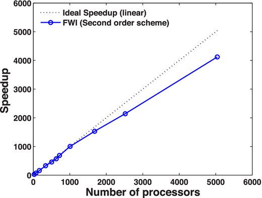
Speedup from parallel processing for a fixed-sized inverse problem (129 × 40 × 47).
4 SYNTHETIC EXAMPLES
In this section, we present several numerical examples of 3-D FWI to validate the algorithm and to give some estimation of the computing cost of the approach. The inverted wavefields—including refractions, turning waves, and reflections—are accounted for simultaneously in the inversion. Synthetic data were generated by the Laplace–Fourier domain FD modelling technique (Petrov & Newman 2012) in conjunction with perfectly matched layers (PML; Hastings et al.1996; Kim & Pasciak 2010) and free-surface boundary conditions (Gottschammer & Olsen 2001). It is the same forward code as embedded in our FWI algorithm. However, we produced the forward data at much greater accuracy than we required for the predicted data within the inversion iteration. The synthetic data were generated using significantly smaller solution tolerances in the Krylov iterations (∼3 orders) than the tolerances employed within inversion for computing data predictions. For inversion, we use noise-free data obtained with the second-order scheme. All examples were computed on CRAY XE6 and CRAY XC30 at the National Energy Research Scientific Computing (NERSC) Center.
4.1 Inclusion model
First, we apply 3-D FWI to the simple velocity model composed of a homogeneous background with an inclusion. Velocities in the background medium are 2150 m s−1 for the S-wave and 4250 m s−1 for the P wave, with background density 2300 kg m–3. The inclusion consists of prisms with 1800 m s−1 for S-wave velocity, 3600 m s−1 for P-wave velocity and 2100 kg m–3 for density. For demonstration of the method sensitivity we used a general case of different S and P-waves space distributions (Figs 4a and b): assigned to the same prism but rotated about the Z-axis by 90°. Consequently, for the P wave, the size of inclusion is defined by |$L_x^p = 20\;{\rm m},\;L_y^p = 30\;{\rm m},\;L_z^p = 20\;{\rm m}$|, while for the S wave it is |$L_x^S = 30\;{\rm m},\;L_y^S = 20\;{\rm m},\;L_z^S = 20\;{\rm m}$|. The density has the same distribution as the P velocity.
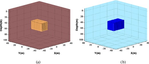
The synthetic example used to test the inversion algorithm (a) P velocity (background – 4250 m s−1, 3600 m s−1 – inclusion) and (b) S velocity (background – 2100 m s−1, 1800 m s−1 – inclusion).
Twelve wells surround the target with 14 horizontal xy-directed point dipole sources at 6 m interval straddling the target (Fig. 5). All three components of the wavefields were calculated in all other wells at 6 m intervals, excluding the source well.
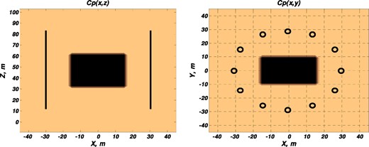
The synthetic example with wellbores positions and P-velocity inclusion geometry.
The model is discretized on a 46 × 46 × 57 grid with 2 m cubic cells, with PML layers spread along five grid cells on each side and in each direction. The inverted frequencies are 30, 50, 70, 100 and 140 Hz which were determined using principles described in (Sirgue & Pratt 2004). As the model and distances between wells are not large, the iterative solution of the forward problem (6) is sufficiently fast for all range of frequencies. So here, we used only one Laplace damping parameter σ = 1 s−1 which provides a good convergence of iterative solution and a small difference from pure Fourier image. Since the low frequencies (30 and 50 Hz) data are used in the inversion process, it is not necessity to use large damping parameters for additional smoothing of solutions. The initial model was the homogeneous media with background P and S velocities and the density.
In total, the data consist of 25 088 source–receiver pairs, with the inversion domain consisting of 120 612 cells and including PML layers. The inversion was performed with unweighted data, that is, using E = I in eq. (1), where I is the identity matrix.
The recovered image in Fig. 6 shows the location, geometry, and values of inclusion fairly well. Relative error for the P-wave velocity values is less than 1 per cent, for the S wave less than 2.5 per cent, and about 5 per cent for density. Unlike the other two parameters the density is very sensitive to the sequence of the Laplace–Fourier domain inversion process, and it is very hard to estimate using classical FWI theory. An acceptable density distribution is obtained only when the inversion process is begun at the lowest frequency data of 30 Hz.
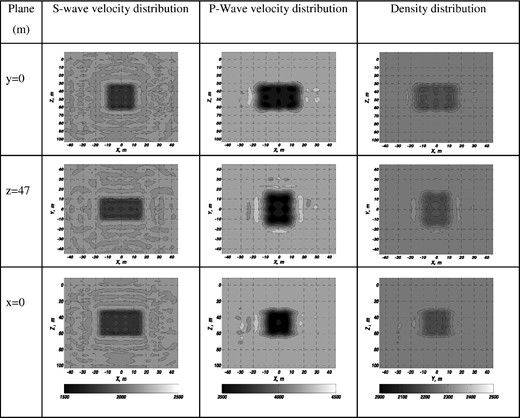
Reconstructed S- and P-wave velocities and the density for the synthetic example illustrated in Fig. 4 for different image slices at x = 0 m, y = 0 m, z = 47 m.
Readers interested in this problem can find a discussion about strategy for density reconstruction in work (Jeong et al.2012 and references therein). Because results of inversion are not so sensitive to density parameter as for shear and bulk moduli one can use some analytical relation between density and P- or S-wave velocities (Gardner et al.1974; Dey & Stewart 1997), which we will do in the next examples.
4.2 Layered model
In the next example, we consider the 3-D inversion of a 2-D elastic medium for a data set collected using a cross-well measurement setup (Habashy et al.2011). The true S- and P-wave velocities are given in Figs 7(a) and (b), with the size of the inversion domain 76 m × 76 m × 200 m. Only part of the inversion domain is shown in Fig. 7; the cells outside this region are used to keep the boundary of the inversion domain at a distance. Our model consists of several layers that deviate from the horizontal and the water-injection region located between z = 38 m and z = 50 m. The survey uses two wells located at x = 24 m, y = 0 m and x = −24 m, y = 0 m, with 30 point (x and y)-directed dipole sources in the first well and 30 receivers in the other, and vice versa. Data consist of the two components (x and z) of the displacement velocity fields, with synthetic data generated by solving the forward problem numerically using a 3-D FD approach with the second-order scheme. In the inversion, we used unweighted data at 50, 70, 100, 140, 200 and 280 Hz; the damping constant was set at 1 s−1, as in the previous example. FD cell size is 2 m for frequencies 50–140 Hz and 1 m for 140–280 Hz; thus, in the simulation, 30 × 30 × 72 or 50 × 50 × 135 meshes are used, respectively.
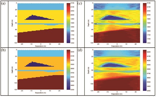
The true (a–b) and the inverted (c–d) distributions of (a, c) S-wave velocity (m s–1) and (b, d) P-wave velocity (m s–1).
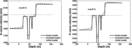
The vertical S, P-wave velocity profiles for the true, inverted and initial models.
4.3 Marmousi model
In the final example, we use the truncated Marmousi-2 elastic model (Martin et al.2002; Xiong et al.2013) to test our 3-D inverse modelling algorithm. Figs 9(a) and (b) shows P- and S-wave velocities of the Marmousi-2 model, where portions of the left- and right-hand side, along with part of the water layer, are removed from the original model. This model is considered to be 2-D where it is invariant along its strike direction, denoted by the y-axis. The dimension of the inversion domain is 5.12 km × 1.56 km × 1.84 km and discretized into 129 × 40 × 47 grid cells. The cell size is 40 m × 40 m × 40 m.
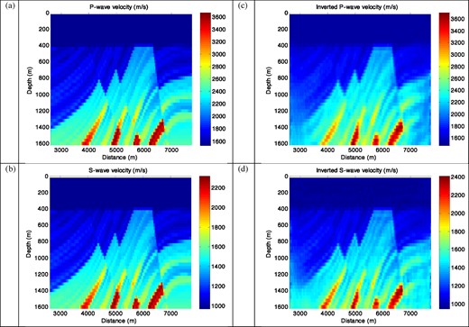
True (a–b) and final results (c–d) after 6 Hz data inversion (a, c) P-wave velocity (m s–1) and (b, d) S-wave velocity (m s–1) of the Marmousi-2 elastic model.
There are 210 dipole point sources uniformly located from x = 2840 to 7480 m along seven lines that span y = −480 to +480 m at 160 m intervals and at a depth of 160 m. A total of 870 receivers locations are equally placed from x = 2800 to 7520 m, along with fifteen lines that span y = −560 to +560 m at 80 m intervals; the inline y = 0 measures two components per detector (the x and z components of the velocity displacement field), while the broadside lines have three components per detector (all three x, y and z components of the velocity displacement field). Receiver depth is 320 m, and each source uses all available receivers. Weighted data are used where weights are proportional to the absolute value of the observed velocity field, that is |$ {\bf E} \sim \sqrt {\vert{{\bf d}^{\rm obs}}\vert}$|, to compensate for attenuation and geometric spreading of the observed data with offset. The data are inverted with four different frequency sets, which include 1.5, 3, 5 and 6 Hz. Thus, at 6 Hz, we have at least 5 grid points per wavelength for the shear wave.
For the lowest frequency inversion and largest damping constant, the initial velocity model is composed of linearly increasing functions with depth, with P-wave velocity varying from 1500 to 2200 m s−1 and S-wave velocity varying from 1000 to 1500 m s−1. The density is again defined by the Gardner relationship in eq. (26), with parameter A = 284. We implemented a single-frequency inversion progressing from the lowest frequency to the highest, with reverse loop, as shown in Figs 1(a) and (b). For each complex frequency, we terminated the inversion when the value of the data misfit (normalized data error) en of (3.5) per cent was achieved, or the relative changes in the model parameters between two successive iterations was less than 0.1 per cent.
The best result of the inversion was obtained with a full data set that includes 1.5, 3, 5 and 6 Hz data. Results after the 6 Hz data inversion are shown in Figs 9(c) and (d) and Figs 10 and 11. As the figures show, the inversion generates very good results: not only have we captured the shape of the faults in the central region of the Marmousi model, but we have also revealed significant detail in this region, where the imaged velocities are computed very accurately. These results show that high spatial resolution can be achieved in the velocity models at relatively low frequencies, that is, 6 Hz. In Fig. 10, at a depth of 1300–1450 m, two neighbouring peaks are successfully separated at a distance of slightly less than half a wavelength. The details of the workflow process for the inversion at different frequencies are given on the left-hand side of Table 1. They confirm that the application of a large damping constant at the beginning of the inversion (at fixed frequency) enables reducing the cost of very expensive calculations employing a small damping constant later in the inversion procedure. During this inversion we applied a pre-conditioner based on the diagonal of the pseudo-Hessian matrix suggested by Choi et al. (2008), but it does not fundamentally solve the slow convergence of the inverse iteration.
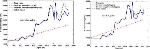
The vertical (a) P-, (b) S-wave velocity profiles for the true, inverted and initial models.
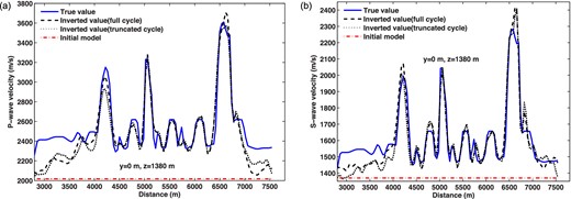
The horizontal (a) P-, (b) S-wave velocity profiles for the true, inverted and initial models.
The details of regular 3-D inverse process showed in Fig. 1(a) for the full data set containing frequencies (1.5, 3, 5, 6 Hz), damping constants (1, 0.5, 0.25 s−1) with the initial inversion Laplace parameter σini = 1 (s−1); fini = 1.5 (Hz) and truncated inverse process (Fig. 1b) containing only large damping constants (from 6.0 to 3.0 s−1) for lower frequencies. Note that sequential ordering is from the top to bottom in the table.
| Sequential downward waveform | Truncated sequential downward | ||||||
|---|---|---|---|---|---|---|---|
| inversion with reverse loops | waveform inversion with reverse | ||||||
| showed in Fig. 1(a) | loop showed in Fig. 1(b) | ||||||
| f (Hz) | σ (s−1) | Number of inverse | Normalized data | σ (s−1) | Number of inverse | Normalized data | Average number of iterations for |
| iterations | error en (per cent) | iterations | error en (per cent) | the forward problem solution | |||
| 1.5 | 6 | 344 | 3.3 | ∼380 | |||
| 3 | 303 | 3.5 | ∼750 | ||||
| 1 | 282 | 4.8 | ∼1300 | ||||
| 0.5 | 180 | 2.3 | ∼4000 | ||||
| 0.25 | 65 | 2.4 | ∼10 000 | ||||
| 3 | 6 | 362 | 2.7 | ∼300 | |||
| 3 | 341 | 3.1 | ∼350 | ||||
| 1 | 642 | 3.8 | 1 | 145 | 2.6 | ∼1700 | |
| 0.5 | 88 | 2.3 | ∼2000 | ||||
| 0.25 | 66 | 2.4 | ∼5000 | ||||
| 5 | 3 | 617 | 3.1 | ∼700 | |||
| 1 | 306 | 2.8 | 1 | 364 | 2.8 | ∼1400 | |
| 0.5 | 148 | 2.3 | 0.5 | 81 | 2.5 | ∼3700 | |
| 0.25 | 92 | 2.4 | 0.25 | 35 | 2.8 | ∼6300 | |
| 1.5 | 0.5 | 78 | 2.3 | ∼2000 | |||
| 3 | 1 | 13 | 2.4 | ∼1000 | |||
| 6 | 0.5 | 126 | 3.2 | 0.5 | 119 | 3.0 | ∼4000 |
| 0.25 | 80 | 3.1 | 0.25 | 60 | 2.7 | ∼10 000 | |
Our simulations show that the truncated cycle of inversion works quite well, obviating the need to perform the full cycle of inversions over all damping constants for all frequencies. In most cases, for low frequencies only large damping constants can be used for inversion, as illustrated in Fig. 1(b). Small damping is applied only to the last steps of the inversion process for high frequencies. One can see (in Figs 10 and 11) that the difference between the full and truncated cycles for the inverted model is slight. The truncated cycle workflow is shown on the right-hand side of Table 1.
A key requirement for successful wide-angle FWI is the presence of low frequencies within the field data. These low frequencies, less than several hertz, are often not easy to identify on time-domain displays, and Fourier amplitude spectra cannot easily distinguish between signal and noise. However, an acceptable signal-to-noise ratio for the Fourier domain may be achieved at the frequencies starting at 3 Hz (Warner et al.2013). Therefore, we have attempted to make the inversion for this case without the lowest frequency of 1.5 Hz present. We used the same configuration of sources–receivers and the initial model, but began the inversion using 3 Hz frequency data with a damping constant σini = 1 (s−1)–the same damping constant used to initiate the inversion in the previous reconstruction. The results are shown in Figs 12(a) and (b). Only the shallow part of the model is acceptable down to a depth of 1000 m. The deepest 3-D structures were not reconstructed, although it is possible to recognize some strongly reflecting interfaces, which are directly connected with P- and S-wave velocity discontinuities. In this case, it appears that the 1.5 Hz frequency information is obviously required for an acceptable reconstruction.
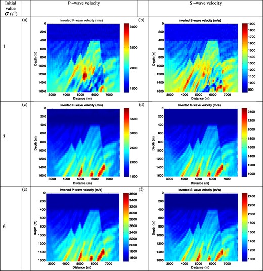
The results after 6 Hz data inversion P-wave velocity (m s–1) and S-wave velocity (m s–1) with the lowest frequency of 3 Hz for different initial damping constants (a, b) σ = 1 (s−1); (c, d) σ = 3 (s−1), (e, f) σ = 6 (s−1).
Nevertheless, even in the absence of this low frequency data, we can still receive an acceptable reconstruction by increasing the damping constant. Figs 12(c) and (d) show the inverted results using σini = 3 (s−1) as an initial damping constant with 3 Hz data. These images are very close to those obtained with the 1.5 Hz frequency data set. All 3-D structures were reconstructed, and the estimated wave velocities are very close to the true values. However, some differences do appear near the left- and right-hand borders of the inversion domain. Increasing σini to 6 (s−1) also provides acceptable results, shown in Figs 12(e) and (f). However, they are worse than the results obtained with σini = 3 (s−1), particularly for the deepest part of the model (below 1600 m). Thus, it appears that wavefield attenuation becomes an issue when the damping constant is set too large. The workflows are presented in Table 2.
The details of 3-D inverse process for the truncated data set containing frequencies (3, 5, 6 Hz) with the initial lowest frequency fini = 3 (Hz) and three different initial damping parameters σini = 1, 3, 6 (s−1). Note once more that sequential ordering is from the top to bottom in the table.
| σini = 1 (s−1) | σini = 3 (s−1) | σini = 6 (s−1) | ||||||||
|---|---|---|---|---|---|---|---|---|---|---|
| f (Hz) | σ (s−1) | Number of | Data error | σ (s−1) | Number of | Data error | σ (s−1) | Number of | Data error | Average number |
| inverse iterations | en (per cent) | inverse iterations | en (per cent) | inverse iterations | en (per cent) | of iterations | ||||
| for forward | ||||||||||
| problem solution | ||||||||||
| 33 | – | – | – | 6 | 1174 | 9.3 | ∼300 | |||
| – | – | – | 4 | 129 | 9.2 | ∼350 | ||||
| 3 | 951 | 2.5 | 3 | 594 | 3.1 | ∼350 | ||||
| 2 | 38 | 2.9 | 2 | 65 | 2.4 | ∼600 | ||||
| 1 | 208 | 3.1 | 1 | 26 | 2.3 | 1 | 23 | 3 | ∼1700 | |
| 0.5 | 100 | 3.2 | 0.5 | 11 | 3.1 | 0.5 | 50 | 2.9 | ∼2300 | |
| 0.25 | 88 | 3.2 | 0.25 | 5 | 3.7 | 0.25 | 17 | 3.5 | ∼5000 | |
| 5 | 3 | 403 | 3.2 | 3 | 894 | 3.1 | ∼700 | |||
| 2 | 106 | 3.1 | 2 | – | – | ∼1000 | ||||
| 1 | 479 | 3.2 | 1 | 180 | 3.2 | 1 | 256 | 2.7 | ∼1500 | |
| 0.5 | 326 | 3.2 | 0.5 | 107 | 3.1 | 0.5 | 71 | 4.2 | ∼3500 | |
| 0.25 | 262 | 6.2 | 0.25 | 88 | 3.3 | 0.25 | – | – | ∼6000 | |
| 3 | 1 | 29 | 2.4 | – | – | – | ∼1000 | |||
| 66 | – | – | – | 1 | 247 | 3 | ∼2000 | |||
| 0.5 | 337 | 3.6 | 0.5 | 317 | 2.9 | ∼4000 | ||||
| 0.25 | 126 | 3.6 | 0.25 | 48 | 3.6 | ∼10 000 | ||||
Undoubtedly, the use of large Laplace damping constants may essentially help the performance of FWI when low frequency data is lacking, but it cannot replace such data completely. For example, we could not obtain acceptable results using only 5 Hz data for inversion. Our simulation shows that availability of 1.5 Hz data for Marmousi-2 elastic model allows not only obtaining a better reconstruction, but also essentially reducing the number of both forward and inversion iterations (see Tables 1 and 2). In any case, it appears probable that the order of single-frequency inversions with changing damping constants, from the largest to the smallest, is optimal for the inversion scheme when imaging reflection data, and where the forward problem is solved using an iterative method, such as a Krylov solver.
Notwithstanding that the results in Figs 12(c)–(f) were obtained after the inversion of 6 Hz data, we determined that acceptable results could be achieved with just the two-frequency set (3 and 5 Hz). Using 6 Hz data brings best results, but results for a maximum frequency of 5 Hz are still very good. Figs 13(a) and (b) presents the inverted images of P and S velocities distributions obtained with only 3 and 5 Hz data, which should be compared with the result inverted using 1.5, 3, 5 and 6 Hz data and to the exact solution in Fig. 9. The Marmousi model clearly demonstrates that our algorithm based on the sequentially ordered single-frequency inversion in the Laplace–Fourier domain can successfully produce 3-D images of complex structures. As the number of frequencies used for the waveform inversion in the Laplace–Fourier domain is increased (partially at low frequencies), the computation efficiency is also increased. Because the reverse loop implementation is adopted, we can easily perform quality control on the inversion process over all frequencies.
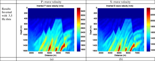
The inversion of (a) P-wave velocity (m s–1) and (b) S-wave velocity (m s–1) with the 3 and 5 Hz data.
5 CONCLUSION
We have presented a 3-D massively parallel elastic waveform inversion algorithm based on an iterative solver, which exploits damping of the wavefield for solution efficiency. In this algorithm, we use the sequentially ordered single-frequency waveform inversion in a multiscale approach. Lowest frequency data is inverted first, followed by higher frequency data. With reflection data, at a fixed frequency, the inversion is performed from the largest Laplace damping constant to the smallest one, and the final model with the smallest damping constant is used as a starting model for the next frequency. To test the model adequacy at all frequencies and prevent the cycle-skipping artefacts used in this recurrence, we allow for the option to resample some lower complex frequency data during the inversion iterations.
We showed that a truncated scheme of inversion workflow, relevant to reflection data, can be very efficiently employed for reducing the most expensive inversion iterations, using small damping constants. This scheme suggests that at higher frequencies, small damping should be used for the final stages of the process, whereas large damping be used only for the lower frequencies.
The advantages of our approach include the efficiency of the forward problem solution provided by the iterative solver under the order as stated above, its efficiency for conducting simulations of relatively modest 3-D FD grids, and the parallelization of the inverse problem resulting from domain and data decompositions.
We have presented several applications of increasing complexity to validate the algorithm on synthetic examples. Some preliminary applications to the fragment of Marmousi model suggest that FWI exploiting damped wavefields can be applied successfully to frequencies up to 6 Hz, and that it is possible to develop accurate 3-D velocity images at a resolution that approaches half the smallest wavelength utilized to image the subsurface: in the case of the Marmousi model, 150 m for a velocity of 3600 m s−1. The final velocity structure was recovered from a simple starting model, and not a smoothed version of the actual velocity model as is common in many FWI implementations. We were able to achieve acceptable results simple using a linearly increasing velocity model with depth.
It is true that our presented results were obtained for modest models and synthetic data without noise. This is because our primary purpose was to elaborate on an effective workflow that allows using FWI with the least computer expense. The next logical step will be to demonstrate the 3-D inversion scheme on large-scale models for data with noise, along with source signature definition. This will be developed in our future work.
This work was carried out at Lawrence Berkeley National Laboratory with funding provided by the U.S. Department of Energy Office of Science and Geothermal Program Office under respective contract numbers DE-AC02-05CH11231 and GT-480010-19823-10. Computational resources were provided by the National Energy Research Scientific Computing (NERSC) Center.
