


Abstract
Various formulations of smoothed particle hydrodynamics (SPH) have been proposed, intended to resolve certain difficulties in the treatment of fluid mixing instabilities. Most have involved changes to the algorithm which either introduces artificial correction terms or violates what is arguably the greatest advantage of SPH over other methods: manifest conservation of energy, entropy, momentum and angular momentum. Here, we show how a class of alternative SPH equations of motion (EOM) can be derived self-consistently from a discrete particle Lagrangian – guaranteeing manifest conservation – in a manner which tremendously improves treatment of these instabilities and contact discontinuities. Saitoh & Makino recently noted that the volume element used to discretize the EOM does not need to explicitly invoke the mass density (as in the ‘standard’ approach); we show how this insight, and the resulting degree of freedom, can be incorporated into the rigorous Lagrangian formulation that retains ideal conservation properties and includes the ‘∇h’ terms that account for variable smoothing lengths. We derive a general EOM for any choice of volume element (particle ‘weights’) and method of determining smoothing lengths. We then specify this to a ‘pressure–entropy formulation’ which resolves problems in the traditional treatment of fluid interfaces. Implementing this in a new version of the gadget code, we show it leads to good performance in mixing experiments (e.g. Kelvin–Helmholtz and ‘blob’ tests). And conservation is maintained even in strong shock/blastwave tests, where formulations without manifest conservation produce large errors. This also improves the treatment of subsonic turbulence and lessens the need for large kernel particle numbers. The code changes are trivial and entail no additional numerical expense. This provides a general framework for self-consistent derivation of different ‘flavours’ of SPH.
INTRODUCTION
Smoothed particle hydrodynamics (SPH) is a method for solving the equations of hydrodynamics (in which Lagrangian discretized mass elements are followed; Gingold & Monaghan 1977; Lucy 1977), which has found widespread application in astrophysical simulations and a range of other fields as well (for recent reviews, see Rosswog 2009; Springel 2010b; Price 2012b).
The popularity of SPH owes to a number of properties: compared to many other methods, it is numerically very robust (stable), trivially allows the tracing of individual fluid elements (Lagrangian), automatically produces improved resolution in high-density regions without the need for any ad hoc pre-specified ‘refinement’ criteria (inherently adaptive), is Galilean-invariant, couples properly and conservatively to N-body gravity schemes, exactly solves the particle continuity equation1 and has excellent conservation properties. The latter character stems from the fact that – unlike Eulerian grid methods – the SPH equations of motion (EOM) can be rigorously and exactly derived from a discretized particle Lagrangian, in a manner that guarantees manifest and simultaneous conservation of energy, entropy, linear momentum and angular momentum (Springel & Hernquist 2002, henceforth S02).
However, there has been considerable discussion in the literature regarding the accuracy with which the most common SPH algorithms capture certain fluid mixing processes [particularly the Kelvin–Helmholtz (KH) instability; see e.g. Morris 1996; Dilts 1999; Ritchie & Thomas 2001; Marri & White 2003; Okamoto et al. 2003; Agertz et al. 2007. Comparison between SPH and Eulerian (grid) methods shows that while agreement is quite good for supersonic flows, strong shock problems and regimes with external forcing (e.g. gravity), ‘standard’ SPH appears to suppress mixing in subsonic, thermal-pressure-dominated regimes associated with contact discontinuities (Kitsionas et al. 2009; Price & Federrath 2010; Bauer & Springel 2012; Sijacki et al. 2012).2 The reason is, in part, that in standard SPH the kernel-smoothed density enters the EOM, and so behaves incorrectly near contact discontinuities (introducing an artificial ‘surface-tension’-like term), where the density is not differentiable.
A variety of ‘flavours’ (alternative formulations of the EOM or kernel estimators) of SPH have been proposed which remedy this (see above and Monaghan 1997; Ritchie & Thomas 2001; Price 2008; Wadsley, Veeravalli & Couchman 2008; Read, Hayfield & Agertz 2010; Abel 2011; Read & Hayfield 2012; García-Senz, Cabezón & Escartín 2012). These approaches share an essential common principle, namely recognizing that the pressure at contact discontinuities must be single-valued (effectively removing the surface tension term). Some of these show great promise. However, many (though not all) of these formulations either introduce additional (potentially unphysical) dissipation terms or explicitly violate the manifest conservation and continuity solutions described above – perhaps the greatest advantages of SPH. This can lead to severe errors in problems with strong shocks or high Mach number flows, limited resolution or much larger gradients between phase boundaries (J. Read, private communication; see also the discussion in Abel 2011; Price 2012b; Read & Hayfield 2012). All of these regimes are inevitable in most astrophysically interesting problems.
Recently, however, Saitoh & Makino (2012, henceforth SM12) pointed out that the essential results of most of these flavours can be derived self-consistently in a manner that does properly conserve energy. The key insight is that the ‘problematic’ inclusion of the density in the EOM (as opposed to some continuous property near contact discontinuities) arises because of the ultimately arbitrary choice of how to discretize the SPH volume element (typically chosen to be ∼mi/ρi). Beginning with an alterative choice of volume element, one can in fact consistently derive a conservative EOM. They propose a specific form of the volume element involving internal energy and pressure, and show that this eliminates the surface tension term and resolves many problems of mixing near contact discontinuities.
In this paper, we develop this approach to provide a rigorous, conservative, Lagrangian basis for the formulation of alternative ‘flavours’ of SPH, and show that this can robustly resolve certain issues in mixing. Although the EOM derived in SM12 conserves energy, it was derived from an ad hoc discretization of the hydrodynamic equations, not the discrete particle Lagrangian. As such it cannot guarantee simultaneous conservation of energy and entropy (as well as momentum and angular momentum). And the EOM they derive is conservative only for constant SPH smoothing lengths (in time and space); to allow for adaptive smoothing (another major motivation for SPH), it is necessary to derive the ‘∇h’ terms which account for their variations. This links the volume elements used for smoothing in a manner that necessitates a Lagrangian derivation. And their derivation depends on explicitly evolving the particle internal energy; there are a number of advantages to adopting entropy-based formulations of the SPH equations instead.
We show here that – allowing for a different initial choice of which thermodynamic volume variable is discretized – an entire extensible class of SPH algorithms can be derived from the discrete particle Lagrangian, and write a general EOM for these methods (equation 12, our key result). We derive specific ‘pressure–energy’ (equation 18) and ‘pressure–entropy’ (equation 21) formulations of the EOM, motivated by the approaches above that endeavour to enforce single-valued SPH pressures near contact discontinuities. We consider these methods in a wide range of idealized and more complex test problems, and show that they simultaneously maintain manifest conservation while tremendously improving the treatment of contact discontinuities and fluid mixing processes.
THE SPH LAGRANGIAN AND EQUATIONS OF MOTION
A fully general derivation
We clearly require some thermodynamic variable to determine P; we can choose ‘which’ to follow, for example internal energy u or entropy A. For a gas which is polytropic under adiabatic evolution (we consider more general cases below), if we follow particle-carried ui, then self-consistency with the thermodynamic equation above requires that we define the pressure in the above equation as Pi = (γ − 1) ui (mi/Δvi); if we follow the entropy Ai we must define Pi = Ai (mi/Δvi)γ.
We stress that |$\Delta \tilde{V}$| does not need to be the same as Δv; one is the effective volume used to evolve the thermodynamics, the other is simply any continuous function used to define the hi, so as to make them differentiable and thus allow us to include the appropriate ‘∇h’ terms in the EOM.
Formulations of the SPH equations
Density–entropy formulation
Note that for adiabatic evolution we require no energy equation, since entropy is followed; for a specific energy defined as |$u \equiv \bar{P}_{i}/[(\gamma -1)\,\bar{\rho }_{i}] = (\gamma -1)^{-1}\,A_{i}\,\bar{\rho }_{i}^{\gamma -1}$|, energy conservation is manifest from the EOM above.
As discussed in Section 1, this formulation is known to have trouble treating certain contact discontinuities. Because the only volumetric quantity that enters is the density, this fails when the densities are no longer differentiable, even when pressure is smooth/constant. Specifically, consider a contact discontinuity, ρ1 c21 = ρ2 c22 (where quantities ‘1’ and ‘2’ are on either side of the discontinuity). As we approach the discontinuity, the kernel-estimated density must trend to some average because it spherically averages over both ‘sides’, ρ → 〈ρ〉, but the particle-carried sound speeds c remain distinct, so the pressure is now multivalued, with a ‘pressure blip’ of magnitude ∼(ρmax/ρmin) Ptrue appearing. This has a gradient across the central smoothing length, causing an artificial, repulsive ‘surface tension’ force that suppresses interpenetration across the discontinuity.
Pressure–energy formulation
There are, however, significant drawbacks to the choice of |$\tilde{x}_{i}=x_{i}$| (|$\Delta \tilde{V}=\Delta V$|), in which case we are implicitly defining h such that |$h_{i}^{3} \propto u_{i}/\bar{P}_{i}$|. This is, by itself, perfectly valid and is easily solved by the same bisector method as in the ‘standard’ (|$\Delta \tilde{V}=m/\rho$|) formulation. However, in practice, the particle ui values vary much more widely than the mi. This leads to some potential problems. First, if there is large variation in ui, convergence in hi can become quite expensive. Secondly, again under circumstances with large disorder, the required hi can become very large, leading to an effective loss of resolution. Thirdly and most problematic, under some circumstances the constraint ϕ can have multiple solutions; in this case if hi ‘jumps’, it is no longer continuously differentiable, and so exact energy conservation is broken.
As discussed in SM12, because the volumetric quantity used in the EOM here is now directly the kernel-estimated pressure (instead of the density), this formulation automatically guarantees that pressure is single-valued at contact discontinuities, and so removes the pressure ‘blip’ and surface tension force. The equations will now be well behaved so long as pressure is smooth. This is true by definition in contact discontinuities; it is of course not true at shocks, but neither (typically) is the density constant there – so we do not lose any desirable behaviours of the density–entropy formulation. In either case, we require some artificial viscosity to treat shocks.
Pressure–entropy formulation
This formulation is very similar to the pressure–energy formulation (and has the identical advantages of good behaviour at contact discontinuities). The only difference is the free choice of thermodynamic variable. This formulation trivially conserves entropy, and manifestly conserves energy to machine differencing accuracy if constant time-steps are used (the choice of pressure–energy or pressure–entropy formulation can lead to some differences when adaptive time-steps are used, but we show these are generally small). It is largely a matter of convenience and minor computational expense which method is preferred.
When the pressure is smooth and there is good particle order, the fi ≈ 0 here, which means our choice of how to regularize h is unimportant, and no spurious ‘surface tension’ force is introduced. For the choice |$\tilde{x}=1$|, the correction terms remain well behaved even if there is large particle disorder in Ai, critical to stability in simulations when heating/cooling are included and entropy is no longer conserved. Another useful feature here is the following: imagine the case where there is large particle disorder so Pj ≫ Pi and Aj ≫ Ai. Since the A terms enter as multiplicative pre-factors (we can re-write the latter formulation with |$\Delta \tilde{V}=1/\bar{n}_{i}$| in the same manner), their difference does not introduce errors into the sum; gradient errors will arise from differencing the Pi terms, but for γ = 5/3 these enter only as P− 1/5i, so differencing errors are greatly suppressed.
More general cases
In Sections 2.2.1–2.2.3, we simplify by assuming the gas obeys a polytropic equation of state (EOS) under differential adiabatic compression or expansion. We emphasize that this does not exclude the gas undergoing shocks (in which the entropy and energy change according to artificial viscosity), cooling and/or chemical evolution (additional operations to dui in equation 2); these are just handled in an additional, separate step or loop in each time-step (see an example in Section 4.8).
However, some situations call for more complicated EOSs. Consider the case where the pressure of a given particle Pi is an arbitrarily complicated (but single-valued) function g of the thermodynamic volume element Δvi and the local (particle-carried) state variables |${\boldsymbol {a}}_{i} = (a_{i,\,1},\,a_{i,\,2},\ldots ,a_{i,\,m})$|, so |$P_{i} = g(\Delta V_{i},\,{\boldsymbol {a}}_{i})$|. The |${\boldsymbol {a}}$| might include mi and ui or Ai, as in our previous examples, but also information about the chemical state, radiation field, position or velocity, phase, etc., of the gas. Our general form of the EOS in equation (12) made no assumption about the EOS, and still holds. The question is how to determine the appropriate xi and |$\tilde{x}_{i}$| for a ‘pressure formulation’. This requires any xi such that there is a one-to-one mapping between the smoothing kernel sum and the pressure [so that ∇(Δv) vanishes when ∇P does]. We can ensure this by choosing xi to be the solution to the equation |$g(\Delta V_{i} = x_{i},\,{\boldsymbol a}_{i}) = 1$| (i.e. if we were to replace Δvi by xi, which we recall typically has different units, we would obtain a dimensionless Pi = 1). We then define Δvi = xi/yi = xi/∑xj Wij(hi) as usual, and take |$P_{i} = g(\Delta V_{i} = x_{i}/y_{i},\,{\boldsymbol a}_{i})$| in equation (12). We still have full freedom to define |$\tilde{x}_{i}$|; based on the formulations above, we suggest that the simple choice |$\tilde{x}_{i}=1$| is often most stable.
It is straightforward to verify that our choices in both the pressure–energy [Pi = (γ − 1) ui mi/Δvi] and pressure–entropy [Pi = Ai (mi/Δvi)γ] formulations satisfy the condition |$g(\Delta V_{i}=x_{i},\,{\boldsymbol a}_{i})=1$|. These are just special cases of the above with |${\boldsymbol a}_{i}=(m_{i},\,u_{i})$| or (mi, Ai) (and different g), respectively.
A more complicated example might be a case with a chemical potential, such that mi dui|A = −Pi dΔvi + ∑μk dNk, where the k are different species. If the Nk are constant over a differential adiabatic volume change, then this can be treated by any of the above formulations with the chemistry evolved (under the effects of radiation, for example) in a separate step. If the Nk are functions of the volume element Δv, however, then we simply have |$m_{i}\,{\rm d}u_{i} |_{A} \rightarrow -\hat{P}_{i}\,{\rm d}\Delta V_{i}$|, where |$\hat{P}_{i} \equiv P_{i} - \sum \mu _{k}\,(\mathrm{\partial} N_{k} / \mathrm{\partial} \Delta V)$|. Therefore, we can use the EOM in equation (12) with |$P_{i}\rightarrow \hat{P}_{i}$|, and use the approach above to determine the appropriate xi (with |$\tilde{x}_{i}=1$|).
ADDITIONAL SIMULATION INGREDIENTS
Entropy and artificial viscosity
As is standard in SPH, the algorithm is inherently inviscid and some artificial viscosity must be included to properly capture shocks. However, we include a more sophisticated treatment of the artificial viscosity term (as compared to S02 and ‘standard’ gadget; which follow Gingold & Monaghan 1983), following Morris & Monaghan (1997) with a Balsara (1989) switch. This includes a particle-by-particle artificial viscosity that grows rapidly in strong shocks and rapidly decays away from shocks (to a minimum α = 0.05), reducing numerical dissipation by more than an order of magnitude away from shocks compared to the previous constant artificial viscosity prescription. For detailed comparison of the viscosity algorithms, we refer to Cullen & Dehnen (2010).
Thermodynamic evolution and time-step criteria
For all problems discussed here, we employ the gadget adaptive time-step algorithm, which dramatically reduces the computational expense for almost all interesting problems (relative to using a constant simulation time-step). However, as pointed out in Saitoh & Makino (2009) and developed further in Durier & Dalla Vecchia (2012), in problems with very high Mach number shocks/bulk flows, the standard adaptive time-stepping can lead to problems if particles with long time-steps interact suddenly mid-time-step with material evolving on much shorter time-steps. Fortunately, this is easily remedied, and we do so by implementing a time-step limiter identical to that in Durier & Dalla Vecchia (2012). At all times, any active particle informs its neighbours of its time-steps and none are allowed to have a time-step greater than four times that of a neighbour; and whenever a time-step is shortened (or energy is injected in feedback), particles are ‘activated’ and forced to return to the time-step calculation as soon as possible.
Smoothing kernel
Our derivation of the EOM allows for an arbitrary choice of SPH smoothing kernel W, so long as it is differentiable. This choice can have a significant effect on some test problems via its effect on the resolution pressure gradient errors (see e.g. Morris 1996; Dilts 1999; Read et al. 2010, and discussion below). We have experimented with a wide range of possible kernel shapes, following the ∼10 kernels discussed in Fulk & Quinn (1996) and Hongbin & Xin (2005), the triangular kernels proposed in Read et al. (2010) and the variant Wendland kernels proposed in Dehnen & Aly (2012). However, our intention here is not to study SPH kernels; for simplicity, we therefore adopt a standard quintic spline kernel with NNGB = 128 neighbours in all tests shown here (unless otherwise noted). This is the ‘optimal’ spline kernel suggested in both Hongbin & Xin (2005) and Dehnen & Aly (2012), and has effective resolution equal to a cubic spline with 34 neighbours (but significantly higher accuracy). In most cases, we obtain similar results using a lower order cubic spline5 with NNGB = 32; but we discuss where this is not the case. We do not see qualitative improvement in the specific tests here using yet higher order kernels and/or increasing neighbour number as high as NNGB ≈ 500.
Density estimation in density-independent SPH
An estimate of the density is often required for other calculations (e.g. cooling), even if it is not needed for the EOM. This can still be directly estimated from the standard SPH kernel, as ρi above (i.e. a kernel sum with xi = mi). However, in principle, a density could also be inferred or estimated as ρth ≈ mi/Δvi for the thermodynamic Δv ‘pressure formulations’ (i.e. from the combination of the variables |$\bar{P}_{i}$| and Ai or ui). However, in ‘mixed’ regions near contact discontinuities, this will lead to multivalued densities in neighbouring particles (since entropies are still conserved at the particle level). This relates to the fact that the two densities represent physically distinct quantities. The former, direct kernel ρi (xi = mi) is simply the volume-average mean mass density at the particle location. The latter (thermodynamically inferred ρth) is the energy- or entropy-weighted mean mass density (in the pressure–energy or pressure–entropy formulations, respectively), averaged over all neighbours within the kernel. Because the cooling is typically calculated on a particle-by-particle basis, we find the former estimator is more stable and appropriate in most applications. However, there may be situations where alternative weightings for the density estimator are optimal, and a more complete treatment of mixing may require a mechanism for equilibrating entropies inside the kernel and generating mixing entropy.
TEST PROBLEMS
Strong Sedov–Taylor blastwaves
Here, in Figs 1, 2 and 3, we consider an extreme Sedov–Taylor blastwave, with very large Mach number, designed to be a powerful test of conservation. A box of side-length 6 kpc is initially filled with 1283 equal-mass particles at constant density n = 0.5 cm−3 and temperature 10 K; 6.78 × 1046 J of energy is added to the central 64 particles in a top-hat distribution. This triggers a blastwave with initial Mach number ∼1000, which we compare at 20 Myr, where the shock front should be at r ≈ 1.19 kpc. In this test and below, unless otherwise specified, we assume a γ = 5/3 gas EOS.
First (Fig. 1), we compare the ‘fully conservative’ algorithms we derive above. In ‘standard’ SPH (density–entropy formulation; equation 14), the analytic solution is reproduced very well up to the SPH smoothing/resolution limit. The narrow shock jump is not perfectly resolved, for example, but averaged over the same smoothing, the agreement is excellent between analytic solution and mean particle values. There is also some scatter in particle properties (most notably velocity), but it is generally narrow. The largest deviation from the analytic solution is in the post-shock ‘ringing’ in the velocity field, a well-known effect (which is sensitive to the artificial viscosity prescription). Note that the behaviour at small radii ≲0.5 kpc is noisy simply because the extremely low density means there are no particles here. As expected, the conservation properties are excellent as well; energy is conserved to a part in ∼104; similar conservation is obtained for entropy, energy, momentum and angular momentum. In fact, the conservation errors are overwhelmingly dominated by the adaptive time-stepping scheme (which violates conservation by not always evolving mutually interacting particles at the same time-steps), not the formulation of the EOM. If we simply force constant, global time-steps, the conservation errors are reduced to machine accuracy (however, this comes at great numerical expense).6
To compare, the pressure–energy formulation [xi = (γ − 1) Ui as equation (18), using the neighbour number density volume element |$\tilde{x}_{i}=1$| to define h] agrees very well, and also gives excellent conservation. The particle noise/scatter is slightly larger, most notably in the post-shock temperature. This occurs because of some ‘mixing’ of thermal properties in the kernel average from higher energy particles. However, the post-shock ringing in the velocity solution (although still present) is reduced.
The pressure–entropy formulation (xi = mi A1/γi, with |$\tilde{x}_{i}=1$|, equation 21) is essentially identical to the pressure–energy formulation here (the slightly better conservation owes to how the sound speeds enter the time-step signalling scheme). This is not surprising – the two represent essentially identical information but just choose to explicitly follow different thermodynamic variables.
As discussed in Section 2.1, the EOM for the pressure–energy and pressure–entropy formulations take a simpler form if we assume |$\tilde{x}_{i}=x_{i}$|, as in standard SPH, but this can lead to problems. We show that here, by considering these implementations (equations 15 and 20 for the pressure–energy and pressure–entropy formulations, respectively). Recall these are still fully conservative Lagrangian formulations; as a result, we still see good energy conservation. However, forcing the smoothing lengths to evolve not just with particle number density but with local thermodynamic quantities leads to occasional enormous ‘supersmoothing’ that is both computationally expensive and introduces enormous numerical diffusion. We see that here, where the upper envelope of particles and even the mean are biased in the pre-shock medium (information from the post-shock region has clearly been oversmoothed into the regions here). Although some mean and post-shock quantities are well behaved, this algorithm has introduced far too much numerical mixing.
We see in Fig. 2 that it is also instructive to see what happens if we drop the ∇h terms in these formations (returning to |$\tilde{x}_{i}=1$|). The EOM will now violate manifest energy conservation to the level that the smoothing lengths vary over an individual smoothing length (in a smooth medium, this correction should vanish at infinite resolution, but it will never vanish in shocks if variable h is allowed). Indeed, we now see order-unity energy errors. Although the qualitative solution appears similar, the pressure–energy and pressure–entropy solutions gain and lose energy, respectively, and so the shock is simply in the wrong position. This occurs in other, similar non-conservative formulations as well [e.g. see the discussion of problems with Ritchie & Thomas (2001) and ‘OSPH’ methods in Read & Hayfield (2012, appendix A)].
Finally, we consider an algorithm which is manifestly non-conservative. Specifically, we consider the Morris (1996) formulation of the pressure derivative, where the kernel sum for the EOM is over (Pj − Pi)/(ρi ρj) ∇Wij. This is very similar (although not identical) to the EOM proposed in Abel (2011) as well. It is possible to show that this formulation actually eliminates the leading-order gradient errors associated with the ‘standard’ SPH EOM (see e.g. Price 2012b). However, the cost is manifest resolution-level violation of conservation (of energy, momentum and entropy). If we adopt our standard initial conditions with this algorithm, we see that the conservation errors grow exponentially and quickly swamp the real solution. The problem, as described in Price (2012b), is in the non-linear terms that maintain particle order in SPH.7
Sod shock tube
Fig. 4 shows the results of a standard 3D Sod shock tube test. We initialize a period domain with lengths 2, 1/8, 1/8 in the x, y, z directions, 5 × 10⁴ particles, γ = 5/3, zero initial velocities, densities ρ = 1, 0.25 and pressures P = 1, 0.22 in the left/right halves of the x domain. In Fig. 4, we compare the results from both standard density–entropy SPH and the pressure–entropy formulation (with |$\tilde{x}_{i}=1$|) at time t = 0.1. The median particle values agree well with the exact solution in both cases. As expected and seen in the Sedov case, the density and pressure discontinuities are smoothed by the SPH smoothing and artificial viscosity but otherwise well behaved. The pressure discontinuity is slightly more smoothed by direct kernel averaging in the pressure–entropy case, but the difference is small.
![Strong Sedov–Taylor blastwave test. We compare the solution at fixed time and resolution, with different SPH algorithms discussed in the text. We plot radial velocity, density and temperature (for clarity, we plot the median and 1–99 per cent interval of particle values binned in radial intervals Δr = 0.01), with the analytic solution. We measure the accuracy of energy conservation δE/E ≡ |E(t) − E(t = 0)|/E(t = 0). Left: standard SPH (density–entropy; $x_{i}=\tilde{x}_{i}=m_{i}$); equation (14). Centre: Lagrangian pressure–energy formulation [xi = (γ − 1) Ui] with particle number density based smoothing lengths ($\tilde{x}_{i}=1$); equation (18). Right: Lagrangian pressure–entropy formulation (xi = mi A1/γi) with particle number density based smoothing lengths ($\tilde{x}_{i}=1$); equation (21). Conservation and accuracy are excellent up to the resolution limits (lack of particles dominates the noise at small radii), in all three algorithms. The pressure formulations slightly increase the particle scatter in temperature, but reduce the post-shock ‘ringing’ of the velocity solution. Conservation errors in all three cases are overwhelmingly dominated by the adaptive time-steps, not the EOM.](https://oup.silverchair-cdn.com/oup/backfile/Content_public/Journal/mnras/428/4/10.1093_mnras_sts210/1/m_sts210fig1.jpeg?Expires=1716410334&Signature=JHkiYtJixV4AECeubs6zN7Wux60JrNVGN2RN8MYXFNrnUD9kg87YEJxZ5GSMBch8bJxfRGjnpnZx~5V04LHFosVrnnAoC3YM6VyLFTEqSJTF6zkckvdj3fgydsV0Hl8D1RgsROIxsK5L2vydV8qBBz5hRXUUaUGmYVlXz5O~TSx2GaZMy92uCaxCTcpxcY6xOc4pg2awhLzpRTWPQOdWoKVtSihlhGVaf5N57PaDXRMEEvRGeoL6jiSzJoBnETFYAmfwhGfCDSQM28ZcHYoLOoWCvdCQpv8~kh-uoGtw5W2X9-1npz0omO4ocQVBjntUtbd7UlXfLzlA1Z6B4dmAZA__&Key-Pair-Id=APKAIE5G5CRDK6RD3PGA)
Strong Sedov–Taylor blastwave test. We compare the solution at fixed time and resolution, with different SPH algorithms discussed in the text. We plot radial velocity, density and temperature (for clarity, we plot the median and 1–99 per cent interval of particle values binned in radial intervals Δr = 0.01), with the analytic solution. We measure the accuracy of energy conservation δE/E ≡ |E(t) − E(t = 0)|/E(t = 0). Left: standard SPH (density–entropy; |$x_{i}=\tilde{x}_{i}=m_{i}$|); equation (14). Centre: Lagrangian pressure–energy formulation [xi = (γ − 1) Ui] with particle number density based smoothing lengths (|$\tilde{x}_{i}=1$|); equation (18). Right: Lagrangian pressure–entropy formulation (xi = mi A1/γi) with particle number density based smoothing lengths (|$\tilde{x}_{i}=1$|); equation (21). Conservation and accuracy are excellent up to the resolution limits (lack of particles dominates the noise at small radii), in all three algorithms. The pressure formulations slightly increase the particle scatter in temperature, but reduce the post-shock ‘ringing’ of the velocity solution. Conservation errors in all three cases are overwhelmingly dominated by the adaptive time-steps, not the EOM.
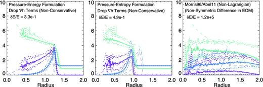
As Fig. 1, but for SPH equations that are not explicitly conservative. Top: pressure–energy formulation without the ∇h terms (fi = 1 in equation 15). Variations in h now cause order-unity energy conservation errors, leading to the shock being in the wrong position. Middle: pressure–entropy formulation without the ∇h terms. Again order-unity conservation errors appear and the shock evolves incorrectly. Bottom: non-Lagrangian SPH as considered in Morris (1996) and Abel (2011); this algorithm minimizes linear pressure errors and removes the surface tension term, but violates conservation of energy and momentum. Conservation errors grow exponentially and dominate the solution.
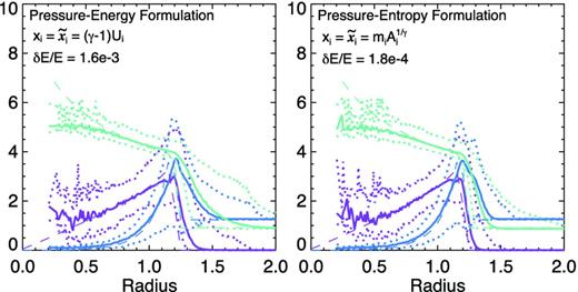
As Fig. 1, with explicitly conservative equations, but different choices of |$\tilde{x}_{i}$| (how to regularize the hi). Top: Lagrangian pressure–energy formulation with |$\tilde{x}_{i}=x_{i}$| (equation 15). Although conservation is maintained, this choice of |$\tilde{x}_{i}$| leads to enormous numerical diffusion and particle disorder (‘spreading’ the shock location over a large radius and affecting the pre-shock gas). Bottom: Lagrangian pressure–entropy formulation with |$\tilde{x}_{i}=x_{i}$| (equation 20). Again, this leads to severe diffusion.
If we zoom in on the pressure profile near the contact discontinuity at x ≈ 0.44 (where the exact solution is P = constant), we see the ‘pressure blip’ discussed in Section 2.2.1 appears in the density–entropy case. The presence of the smoothed density in the EOM leads to an artificial pressure gradient; this occurs over a couple of SPH smoothing lengths with a fractional amplitude of ∼10 per cent. However, it is clearly above the particle noise threshold, and we show below that it has significant effects. In the pressure–entropy formulation, this is almost completely eliminated (at least reduced to the noise level), whether we choose |$\tilde{x}_{i}=1$| or |$\tilde{x}_{i}=x_{i}$|.
We have also repeated the 1D shock tube tests in SM12; our results are generally indistinguishable from their figs 2–4.
Hydrostatic equilibrium/surface tension test
Here we consider a simple test following Cha, Inutsuka & Nayakshin (2010), Heß & Springel (2010) and SM12, which allows us to see the consequences of the ‘surface tension’ effect discussed in Section 1. We initialize a 2D fluid in a square of length L = 1 (with period boundaries) and constant pressure P = 3.75, polytropic γ = 5/3 and density ρ = 4 ρ0 within a central square of length L = 1/2 and ρ = ρ0 = 7/4 outside. We use 2562 total particles, though the results are similar for as few as ∼502.
Fig. 5 shows the resulting system at t = 0, and evolved to t = 3, in the ‘standard’ density–entropy formalism (equation 14) and pressure–entropy formulation (equation 21; it makes little difference for this test whether we adopt |$\tilde{x}_{i}=x_{i}$| or |$\tilde{x}_{i}=1$|). This should be a stable configuration. However, the density–entropy case behaves as a system with physical surface tension; a repulsive force appears on either side of the contact discontinuity from the ‘pressure blip’, opening the gap in the plot which then deforms the square to minimize the surface area of the contact discontinuity. It converges to a stable circle after a few relaxation oscillations. In the pressure–entropy case, the square remains stable for the duration of the runs we consider (t = 50). There is a slight ‘rounding’ of the corners, but this occurs quickly (t < 1) and then stabilizes; it appears to be a direct consequence of the smoothing kernel. These results are identical to those in SM12, for the pressure–energy formulation (with no ∇h terms).
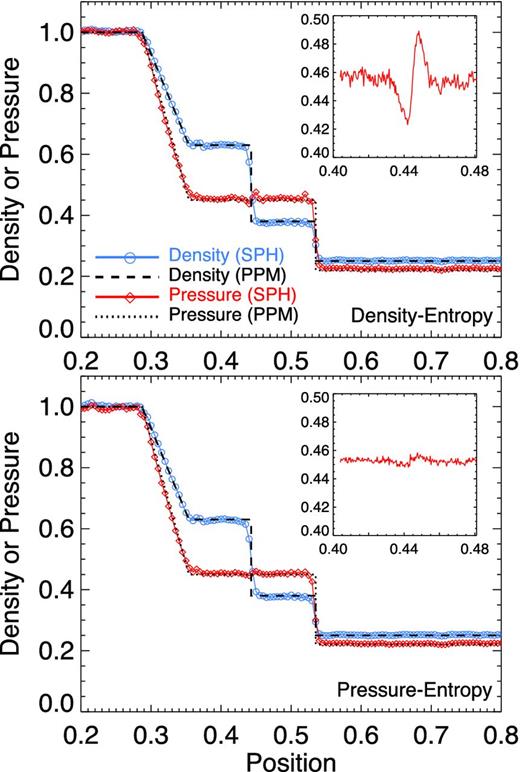
Sod shock tube in three dimensions at time t = 0.1. We show the median particle density and pressure along the long x-axis position (binned as Fig. 1), compared to the reference solution from a piecewise parabolic method (PPM) solver. Inset shows the pressure profile binned in much smaller intervals around the location of the contact discontinuity (x ≈ 0.44), where the pressure should be constant. Top: standard (density–entropy) SPH. The exact solution is generally reproduced well up to SPH smoothing, as Fig. 1, but a ‘pressure blip’ with an artificial gradient appears near the contact discontinuity. Bottom: pressure–entropy SPH (equation 21, with |$\tilde{x}_{i}=1$| for the reasons in Fig. 3). The pressure blip is reduced to particle noise level, while the agreement elsewhere with the PPM result remains.
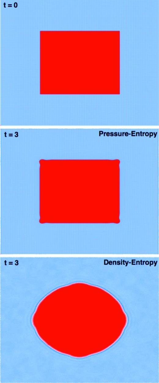
Density (red =4x blue) in a hydrostatic equilibrium test, with uniform pressure and no external forces. Top: initial condition. Middle: system evolved to time t = 3 in the pressure–entropy formulation (equation 21). The square evolves stably (the small corner rounding stems from the smoothing kernel). Bottom: time t = 3 in standard (density–entropy) SPH. The ‘pressure blip’ around the contact discontinuity (Fig. 4) manifests as an effective surface tension, opening a smoothing-length gap between the two fluids, and gradually deforming the square into a circle.
Kelvin-Helmholtz instabilities
We next consider a (3D) KH test. The initial conditions are taken from the Wengen multiphase test suite8 and described in Agertz et al. (2007) and Read et al. (2010). Briefly, in a periodic box with size 256, 256, 16 kpc in the x, y, z directions (centred on 0, 0, 0), respectively, ≈106 equal-mass particles are initialized in a cubic lattice, with density, temperature and x-velocity of ρ1, T1, v1 for |y| < 4 and of ρ2, T2, v2 for |y| > 4, with ρ2 = 0.5 ρ1, T2 = 2.0 T1, v2 = −v1 = 40 km s−1. The values for T1 are chosen so the sound speed cs, 2 ≈ 8 |v2|; the system has constant initial pressure. To trigger instabilities, a sinusoidal velocity perturbation is applied to vy near the boundary, with amplitude δvy = 4 km s−1 and wavelength λ = 128 kpc.
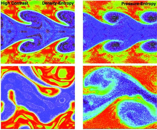
Fig. 6 compares the resulting behaviour in the ‘standard’ density–entropy formulation of SPH (equation 14) and the pressure–entropy formulation (equation 21) proposed here. Because of the severe diffusion seen in the Sedov test associated with the choice of |$x_{i}=\tilde{x}_{i}$| for the pressure–entropy formulation, we focus on the formulation with the ‘neighbour number density’ volume element used to define h, i.e. |$\tilde{x}_{i}=1$|. However, for the subsonic, pressure-equilibrium systems simulated in this test, the choice of |$\tilde{x}_{i}$| makes little difference (highlighting the importance of our strong shock tests). We also do not further separately consider the pressure–energy formulation, as it gives very similar results in our subsequent tests. As expected from the discussion in Section 1, the density–entropy formulation poorly captures the KH instability. The surface tension term forms a sharp boundary layer between the two phases, which suppresses all the small-wavelength mixing and leads at late times to the breakup of the ‘rolls’. This ultimately produces blobs that resemble an oil-and-water morphology (a system with physical surface tension).
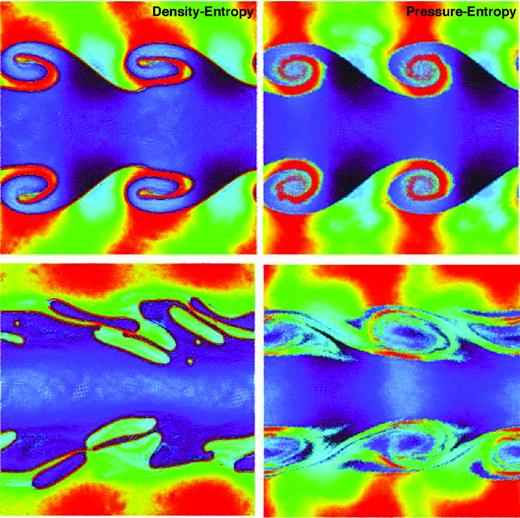
Specific entropy map of KH instabilities at time two times the linear KH growth time-scale τKH (top) and at 8 τKH (bottom). Left: standard (density–entropy) SPH. Note the ‘surface layer’ surrounding the curls and the breakup into oil-and-water style blobs at later times. Right: pressure–entropy formulation (|$\tilde{x}_{i}=1$|).
In the pressure–entropy formulation, however, the behaviour is dramatically improved. The long-wavelength mode grows on the correct (linear) KH time-scale, but we can also plainly see the growth of modes at all wavelengths (along the ‘edge’ of the density surface) down to the kernel scale. At later times, we resolve ∼3–5 full ‘wraps’ of the rolls while the standard SPH solution breaks up. Most important, there is obviously actual mixing occurring ‘inside’ the rolls. Direct comparison to high-resolution results from grid codes (both fixed-grid and adaptive mesh solutions) as well as Godunov SPH and moving-mesh methods, using identical initial conditions, shows that the result here is quite similar (compare e.g. Read et al. 2010 fig. 6, or Murante et al. 2011 figs 5–9).
In Fig. 7, we repeat this experiment with the pressure–entropy formulation, but replace our standard treatment of artificial viscosity (see Section 3.1) with a more simplified treatment (using a constant artificial viscosity for all particles and times); the latter is known to produce significantly more numerical dissipation away from shocks. Although it is well known that this can produce significant differences in some situations (e.g. subsonic turbulence and rotating shear flows; see Cullen & Dehnen 2010; Price & Federrath 2010; Bauer & Springel 2012), it has little effect on this particular test. This owes in part to the implementation of the Balsara (1989) switch in both cases, which reduces the artificial shear viscosity; without this, we see significantly greater damping of shear motions.
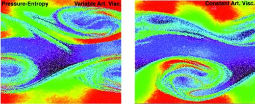
Comparison of the KH behaviour at t = 12 τKH on artificial viscosity in the pressure–entropy formulation. Left: our standard, particle-by-particle time-dependent artificial viscosity following Morris & Monaghan 1997. Right: the original gadget simplified constant artificial viscosity prescription (as Gingold & Monaghan 1983 with a Balsara 1989 switch). Although very important for some behaviours, it has little effect on KH instabilities within this formulation.
In Fig. 8, we again repeat this experiment with the pressure–entropy formulation, but vary the smoothing kernel. We compare two spline kernels, for the neighbour numbers advocated in Price (2012b) and Dehnen & Aly (2012), and the ‘core-triangle’ kernels with sharp central peaks, proposed in Read et al. (2010). For the standard initial conditions here, we see only subtle differences over a wide range from even the simplest kernel with 32 neighbours up through more than an order of magnitude higher neighbour number.9 By explicitly eliminating the ‘surface tension’ term, while maintaining exact conservation, the pressure–entropy formulation appears to significantly reduce the importance of kernel-level pressure gradient errors in obtaining the correct KH solution (compare, e.g., the more significant kernel dependence found for standard but non-conservative density–entropy SPH in Read et al. 2010, figs 4 and 6). We have also tested the Wendland kernels proposed in Dehnen & Aly (2012) and find (as they do) essentially identical performance to our spline results for the neighbour numbers here (although the kernels proposed there show greatly improved stability properties at higher neighbour number).
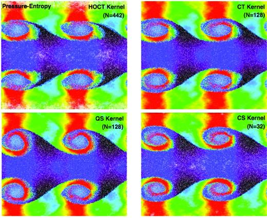
Comparison of the KH behaviour at t = 3 τKH on the smoothing kernel in the pressure–entropy formulation. Top left: quartic core-triangle kernel with neighbour number NNGB = 442 from Read et al. (2010). Top right: cubic core-triangle with NNGB = 128. Bottom left: quintic spline with NNGB = 128. Bottom right: cubic spline with NNGB = 32.
However, in Fig. 9 we again examine the effects of different kernels (with the pressure–entropy formulation), but with different initial conditions. We reduce the particle number, shear velocity and initial perturbation amplitude by factors of 2 and double the initial sound speed; these changes all reduce the magnitude of the initial KH instability and its growth rate, relative to the particle noise and error terms stemming from the kernel sum in the SPH pressure gradients that enter the EOM. This is designed to be challenging (even for grid codes). With this much weaker seeding and noisier particle distribution, we begin to see a dependence on the smoothing kernel. The simplest NNGB = 32 cubic spline, with the smallest neighbour number, leads to particle noise in the pressure gradients comparable to the actual signal. While the instability is still (barely) captured, the rolls are ‘too thin’ and end up being sheared before they reach the proper height and can wrap appropriately. However, our standard quintic spline with NNGB = 128 performs well, recovering all the key behaviours (note that the non-linear behaviour is different here than in the previous test, as it should be for the different pressure and shear velocities). Going to still higher resolution or varying the kernel at higher NNGB gives well-converged results at this point.
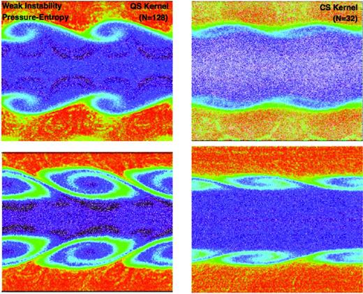
Comparison of KH behaviour with different initial conditions in the pressure–entropy formulation at t ≈ 1 τKH (top) and t ≈ 3 τKH (bottom) on smoothing kernel (left: quintic spline with NNGB = 128; right: cubic spline with NNGB = 32). Compared to Figs 6–8, we modify the initial conditions by multiplying the particle number, density, sound speed, pressure, shear velocity and initial perturbation amplitude by factors of =0.5, 2.0, 2.0, 8.0, 0.5 and 0.5, respectively. All of these changes increase the ratio of particle noise and pressure gradient errors relative to the KH growth. In this limit, the cubic spline with NNGB = 32, which involves larger gradient errors, is barely able to capture the instability; however, the quintic spline with NNGB = 128 does well. ‘Standard’ SPH completely fails to develop any ‘curls’ in this limit.
In Fig. 10, we repeat our KH test again but multiply the initial density contrast by a factor of 10, and instead of using constant-mass particles we use particles with masses a factor of 4 larger in the high-density region. As discussed in Read & Hayfield (2012), many proposed alternative formulations of SPH, designed to improve fluid mixing, fail in this regime (see e.g. fig 6 in Read et al. 2010, and figs A1 and E1 in Read & Hayfield 2012). And we see an even more pronounced ‘boundary layer’ separating the phases in the standard density–entropy SPH formulation. This occurs because the higher density contrast exacerbates any (even small residual) surface tension term, and the multimass particles increase particle disorder and leading-order errors in the pressure gradient estimator. Multimass particles also make it critical to have a well-behaved criterion for smoothing lengths, and increase the errors from neglecting ∇h terms. However, we see that the pressure–entropy formulation remains well behaved in this case. There is some increased hint of ‘gloopiness’ as the instability transitions between linear and non-linear growth, but at least some of this is because of the (correct) slower growth of the small-wavelength modes.
Comparison of KH instabilities at t ≈ 2 τKH ( top) and t ≈ 10 τKH (bottom), for the ‘standard’ (density–entropy) SPH (left) and pressure–entropy (right; with |$\tilde{x}_{i}=1$|) SPH formulations. The initial conditions are as Fig. 6, but the initial density contrast is increased from a factor of 2 to a factor of 20, with the initial particles no longer being equal mass but four times more massive in the initial high-density region. Sharp boundary layers that lead to ‘gloopy’ morphology are evident in standard SPH. In pressure–entropy SPH, it remains well behaved, although hints of ‘gloopiness’ appear in the transition between linear growth and fully non-linear instability.
Finally, it is worth noting (though perhaps as more of a curiosity) that the ‘poor’ solution of the density–entropy formulation in the cases above looks very similar to the ‘correct’ solution for a modestly magnetized medium (with some field component parallel to the shear or tangled; see e.g. Frank et al. 1996, and references therein). This occurs because, if we consider the linear perturbation analysis of the KH instability, the ‘incorrect’ surface tension force here is (for the initial linear stage) almost mathematically identical to a ‘correct’ magnetic tension term for parallel fields with strength β ∼ 1.
Rayleigh–Taylor instabilities
We now consider the Rayleigh–Taylor (RT) instability, with initial conditions from Abel (2011). In a 2D slice with 5122 particles and 0 < x < 1/2 (periodic boundaries) and 0 < y < 1 (reflecting boundary with particles at initial y < 0.1 or y > 0.9 held fixed), we take γ = 1.4 and initialize a density profile ρ(y) = ρ1 + (ρ2 − ρ1)/(1 + exp [−(y − 0.5)/Δ]), where ρ1 = 1 and ρ2 = 2 are the density ‘below’ and ‘above’ the contact discontinuity, and Δ = 0.025 is its width; initial entropies are assigned so the pressure gradient is in hydrostatic equilibrium with a uniform gravitational acceleration g = −1/2 in the y direction (at the interface, P = ρ2/γ = 10/7 so cs = 1). An initial y-velocity perturbation vy = δvy {1 + cos [8π (x + 1/4)]} {1 + cos [5π (y − 1/2)]}, with δvy = 0.025, is applied in the range 0.3 < y < 0.7.
Fig. 11 shows the resulting evolution as a function of time, in the density–entropy and pressure–entropy formulations. As in SM12, both cases develop the RT instability with a similar linear growth time (slightly slower in the density–entropy case); we find that this is true for all of the kernel variations and both artificial viscosity choices discussed above, as well as for the slightly different (isoentropic) initial conditions used in SM12, also for 10 times smaller initial perturbations (δvy = 0.0025) and for resolutions as low as 50 × 100 particles.10 However, they differ significantly in their non-linear evolution; surface tension in the density–entropy formulation prevents the development of fine structure in the shear flow along the ‘fingers’, obviously very closely related to the behaviour in the KH tests. Pressure–entropy SPH, however, exhibits growth on the correct linear time-scale and non-linear behaviour in agreement with that in Eulerian and moving-mesh schemes (e.g. Springel 2010a).
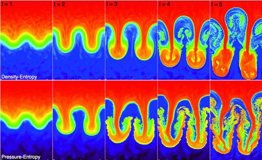
Time evolution of a 2D RT instability (specific entropy map shown). Top: standard (density–entropy) SPH. Bottom: pressure–entropy formulation (|$\tilde{x}_{i}=1$|). The RT instability develops in both cases but the mixing along the rising/sinking surfaces (a KH instability) is suppressed in density–entropy SPH, leading to different non-linear outcomes.
The ‘blob’ test
We next consider the ‘blob’ test, which is designed to test processes of astrophysical interest (e.g. ram-pressure stripping, mixing, KH and RT instabilities in a multiphase medium). Again our initial conditions come from the Wengen test suite and are described in Agertz et al. (2007). Briefly, the initial conditions include a spherical cloud of gas with uniform density in pressure equilibrium with an ambient medium, in a wind tunnel with periodic boundary conditions. The imposed wind has Mach number |$\mathcal {M}=2.7$| and the initial density/temperature ratios are equal to 10. The box is a periodic rectangle with dimensions x, y, z = 2000, 2000, 6000 kpc, with the cloud centred on 0, 0, − 2000 kpc; the 9.6 × 10⁶ particles are equal mass and placed on a lattice.
Fig. 12 shows the resulting morphology of the cloud as a function of time, in the pressure–entropy formulation. Fig. 13 attempts to quantify the rate of cloud disruption following Agertz et al. (2007), who defined a useful standard criterion for measuring the degree of mixing of initially dense blob gas: at each time, we simply measure the total mass in gas with ρ > 0.64 ρc and T < 0.9 Ta (where ρc and Ta are the initial cloud density and ambient temperature). We show the standard SPH (density–entropy) result from that paper, as compared to the prediction from the pressure–entropy formulation here. We also compare the result from the identical test in SM12, using the pressure–energy formulation but without including the ∇h terms in the EOM, as well as the results from a high-resolution run with enzo (O’Shea et al. 2004), a grid code.
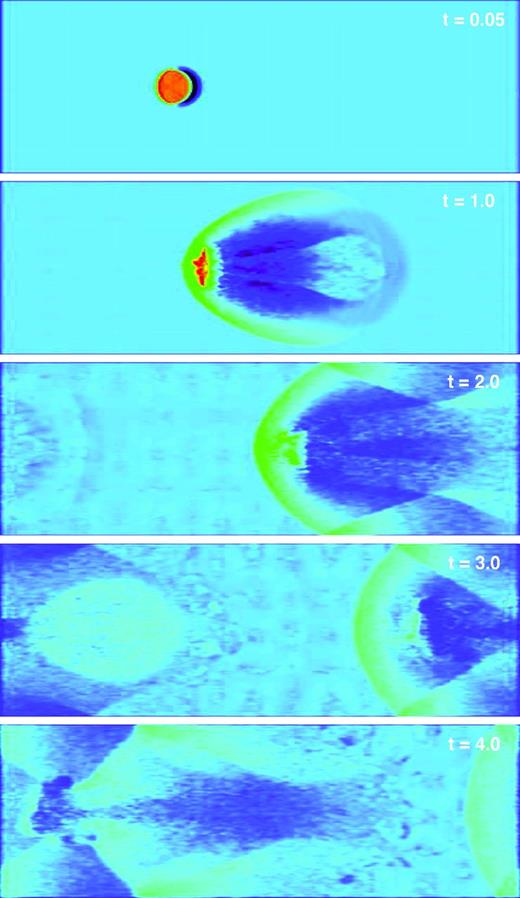
Central density slices in the ‘blob test’ (a high-density, pressure-equilibrium cloud hit by a wind) with the pressure–entropy formulation. Time (in units of the KH growth time) increases from top to bottom. The high-density (red/orange) cloud gas is efficiently mixed by instabilities within a couple cloud crossing times; the morphology and density distribution agree well with grid codes.
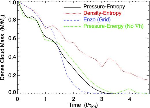
Fraction of the initial cloud in Fig. 12 which remains both cold and dense (i.e. avoids mixing) as a function of time, relative to the KH growth time at the cloud surface. We compare the standard SPH (density–entropy) and pressure–entropy formulations here, as well as the pressure–energy formulation in SM12 (which does not include the ∇h terms) and the results from a high-resolution grid code method (enzo). The grid code and pressure formulations (independent of the ∇h terms) agree reasonably well. Density formulations show slower mixing/stripping.
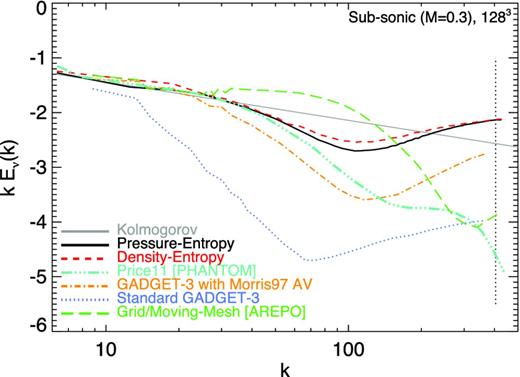
Velocity power spectrum in subsonic (|$\mathcal {M}=0.3$|) driven, isothermal turbulence. Each simulation uses 1283 particles and identical driving. We compare the analytic Kolmogorov inertial-range model to that calculated from our standard density–entropy (equation 14) and pressure–entropy (equation 21) formulations. The mean softening length h is shown as the vertical dotted line. Both do well down to a few softenings, where they first fall below the analytic result (excess dissipation), then rise above (kernel-scale noise). The EOM choice has a weak effect on the results. We compare different SPH algorithms and codes (description in text); agreement is good where the same methods are used. The ‘phantom’ and ‘gadget-3 with Morris97 AV’ use a density–entropy EOM with similar artificial viscosity treatment to our calculations (which dominates the inertial range), but different SPH kernels and power spectrum calculation methods (which dominate the noise at ≲ 3 h). The ‘standard’ gadget-3 calculation uses a constant artificial viscosity and different kernel, and produces almost no inertial range. The arepo calculation considers a grid/moving mesh at the same resolution: deviations from Kolmogorov occur around the resolution limit, but are of a different character.
The wind–cloud interaction generates a bow shock and immediately begins disrupting the cloud via a combination of KH and RT instabilities at its surface. By the middle panel in Fig. 12, there is no visible large concentration of dense material. Compare this to the identical initial conditions run with standard SPH and grid codes in Agertz et al. (2007, their figs 4 and 7). In standard SPH, the cloud is compressed to a ‘pancake’, but the tension term prevents mixing at the surface and so a sizeable fraction survives disruption for large time-scales. In contrast, the predicted morphology of the cloud here agrees very well with that in adaptive mesh codes therein (as well as moving-mesh methods in Sijacki et al. 2012). And quantitatively, we see this in Fig. 13.
However, once again we should note that the solution derived from the density–entropy formulation is remarkably similar to the ‘correct’ solution with magnetic fields with β ≳ 1 (compare e.g. Mac Low et al. 1994; Shin, Stone & Snyder 2008), because the artificial surface tension term acts similarly to magnetic tension.
Subsonic turbulence
Bauer & Springel (2012) present a detailed study of the properties of idealized driven isothermal turbulence in SPH – specifically using gadget-3 with the density–entropy formulation – as compared to moving-mesh and grid methods (in the code arepo; Springel 2010a). Consistent with earlier results, they found that different methods agree well when turbulence is supersonic (e.g. Kitsionas et al. 2009; Price & Federrath 2010). However, when the turbulence is subsonic, they found that density–entropy SPH tended to reproduce a smaller inertial range. However, as discussed there and in Price (2012a), this can depend quite sensitively on the artificial viscosity prescriptions and other numerical details. In Fig. 14 we therefore reproduce the subsonic, driven turbulence experiment from Bauer & Springel (2012) but adopt the pressure–entropy formulation, to test whether it also differs significantly from the results in the density–entropy formulation. We adopt the identical set-up and resolution (A. Bauer, private communication), with the initial conditions and driving algorithm described therein. Briefly, we initialize a box of unit length, density and sound speed with 1283 particles, and drive the turbulence in a narrow range of large-k modes with characteristic Mach number |$\mathcal {M}=0.3$| on the largest scales; unlike our other experiments, the gas is isothermal (γ = 1). We run the experiment to t = 25 (more than sufficient to reach steady state).
We compare the turbulent velocity spectrum measured following Bauer & Springel (2012) (we linearly interpolate the particle-centred velocity values to a uniform grid, Fourier transform each velocity component, and average in bins of fixed |$|{\boldsymbol k}|$| to obtain the kinetic energy power spectrum). The resulting power spectrum is plotted from k ≈ 2π (though k ≲ 10 are affected by the turbulent forcing as well as the finite box size) to k ≈ 500 (a smoothing length h). We compare the pressure–entropy formulation to the results of standard (density–entropy formulation) SPH. The results are nearly identical (although there is slightly more power at intermediate scales in the density–entropy formulation). The results follow the expected Kolmogorov inertial range, until |${\sim }4\,\text{h}$|, where they drop below owing to artificial numerical dissipation; they then rise at ∼2 h, owing to kernel-scale noise (largely from pressure gradient errors).
We can compare this to other SPH results using the identical initial conditions and driving routine. First, consider the results from Bauer & Springel (2012), using ‘standard’ gadget-3 (density–entropy EOM, without the additional algorithm improvements discussed in Section 3) but with an artificial viscosity scheme following Morris & Monaghan (1997) similar (though slightly different) to that adopted here, and the noisier NNGB = 32 cubic spline kernel. We also compare the results from Price (2012a) using a different SPH code (phantom), with the same density–entropy EOM, and an artificial viscosity treatment identical to that here, but using an intermediate kernel (NNGB = 58 cubic spline) and different power spectrum calculation method. As shown there, the artificial viscosity treatment dominates large/intermediate scales. Hence, with identical artificial viscosity, the Price (2012a) result is identical to ours over the inertial range (including the initial ‘drop off’). The smaller scale (≲2–3 h) behaviour is dominated by the kernel choice and method of power spectrum calculation. If we compare ‘standard’ gadget-3 with constant artificial viscosity (Gingold & Monaghan 1983) from Bauer & Springel (2012), we see much more severe excess dissipation and almost no inertial range.
Comparing to the results from arepo in Bauer & Springel (2012) (run either in fixed-grid or in moving-mesh mode, they are nearly identical), we see that the deviations from Kolmogorov there are opposite in sign and quite distinct. In SPH, artificial viscosity produces excess dissipation on larger (resolved) scales, while kernel gradient errors lead to particle noise that boosts the power at the smallest scales. The former (larger scale deviations), being dominated by artificial viscosity, are only indirectly tied to resolution; considering higher resolution runs, we confirm the results in Bauer & Springel (2012) regarding the relatively slow convergence of the high-k spectrum in SPH relative to grid codes. The latter (smaller scale deviations) are related to the conservative nature of the code and its ability to dissipate particle noise (their ‘return’ to and overshoot of the Kolmogorov power law are numerical, rather than physical consequences of a turbulent cascade). In Eulerian approaches, the lack of any but numerical viscosity concentrates the dissipation at the resolution/cell scale, which produces a ‘bottleneck’ of excess power that cannot be dissipated at the larger (marginally resolved) scales; but this scales directly with the resolution.
Stellar feedback in isolated galaxies
Finally, we test our modified algorithm on a fully non-linear system of particular astrophysical interest. Specifically, we re-run one of the star-forming galaxy disc models described in Hopkins, Quataert & Murray (2011b) and a subsequent series of papers (Hopkins et al. 2011a, 2012b; Hopkins, Quataert & Murray 2012a). These simulations include gravity, collisionless stars and dark matter, and gas with a wide range of cooling processes11 from ∼10–109 K, supersonic turbulence, shocks, star formation in resolved giant molecular clouds, and explicit treatment of stellar feedback from Types I and II SNe, stellar winds, photoionization and photoelectric heating, and radiation pressure. Our purpose here is both to test how robust these algorithms are (since many problems with, e.g., non-linear error terms or conservation errors often do not manifest in simple test problems such as those above) and to examine how significant the pure numerical issues of fluid mixing are, relative to, e.g., the previously studied effects of adding/removing different physics in these simulations.
We specifically re-run the ‘SMC’ model (a model of a Small Magellanic Cloud mass, gas-rich isolated dwarf galaxy), at ‘high’ resolution (1 pc softening length) as defined in the papers above, with all the above physical processes included exactly as in Hopkins et al. (2012b), but in one case adopting the density–entropy formulation and in another the pressure–entropy formulation. We choose this model because, of the galaxy types studied therein, it has the largest mass fraction in hot gas and is most strongly affected by thermal feedback mechanisms (e.g. SNe), and as a result is most sensitive to fluid mixing and phase structure. Figs 15–16 compare the visual morphologies and star formation rates (SFRs) from these simulations. Taking into account that the systems are turbulent and non-linear, the morphologies are similar. They differ as one might expect: the pressure–entropy formulation increases mixing along phase boundaries, leading to less sharp divisions between molecular clouds and/or hot, underdense bubbles and the surrounding medium. This also makes the division between the star-forming and ‘extended’ disc less sharp, as it is largely determined by the radius where the cooling rate becomes fast relative to the dynamical time.12
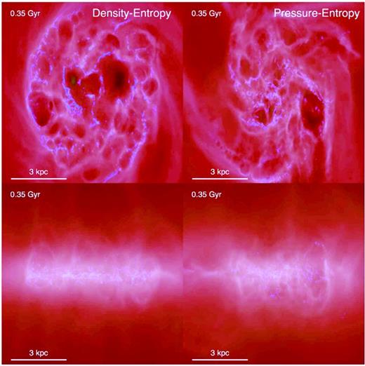
Morphology of the gas in a simulation of a star-forming disc galaxy (an isolated, SMC-mass dwarf) from Hopkins, Quataert & Murray (2012b), following the resolved physics of the interstellar medium (ISM) and stellar feedback explicitly. Brightness encodes projected gas density (logarithmically scaled with ≈6 dex stretch); colour encodes gas temperature with the blue material being T ≲ 1000 K molecular and atomic gas, pink ∼104–105 K warm ionized gas and yellow ≳106 K hot gas. We show the galaxy face-on (top) and edge-on (bottom) after several orbital periods of evolution (during which the galaxy is in quasi-steady state). We compare the identical simulation using the density–entropy (equation 14) and pressure–entropy (equation 21) formulations of SPH. The two are largely similar. There is slightly sharper delineation between phases (e.g. molecular clouds and hot bubbles) in the density–entropy formulation; this includes the sharper transition between the star-forming and outer discs (physically, where the cooling time becomes longer than the dynamical time).
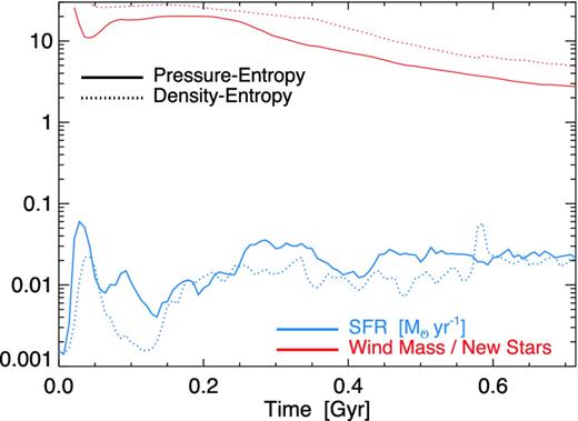
SFR and stellar wind mass-loading (ratio of total unbound gas mass to total new stellar mass formed since the start of the simulation) as a function of time, for the galaxy simulations in Fig. 15. Although stochastic variations in the SFR differ by factors of ∼2–3, the time-averaged SFR is only ∼20 per cent lower in the density–entropy formulation. The wind mass-loading is systematically higher in this case by a factor of ∼1.5–2.0. This stems from increased phase mixing in the pressure–entropy formulation introducing more cold, dense gas into ‘hot’ gas, enhancing its cooling before it can vent out of the disc.
Quantitatively, the time-averaged SFRs differ remarkably little, just ≈20 per cent (with higher SFRs in the pressure–entropy case); this owes to the fact that they are globally set by equilibrium between momentum injection from stellar feedback and dissipation of turbulent energy/momentum on a dynamical time (Hopkins et al. 2012b). The instantaneous rates vary more rapidly and can differ by factors of ∼2–3. We also compare the mass-loading of galactic winds in each simulation, defined as in Hopkins et al. (2012a) as the ratio of total ‘wind mass’ (material with positive Bernoulli parameter, i.e. which will be unbound in the absence of external pressure forces) to new stellar mass formed since the beginning of the simulation. Here the qualitative behaviour is the same but the wind mass-loading is systematically smaller in the pressure–entropy case, by a factor of ∼1.5–2. This is directly related to the higher SFR; both owe to the increased mixing reducing the cooling time of the hot gas bubbles (which provide, for this small galaxy, much of the wind mass). In more massive galaxies, the winds in these simulations are less dominated by hot gas, so the effect will be smaller. These differences (while not negligible) are smaller than those typically caused by adding or removing different feedback mechanisms, or even changing details of their implementation (shown in Hopkins et al. 2012a). For example, removing stellar feedback entirely in this simulation changes the SFR by a factor of ∼50! Integrated over cosmological times, or allowing for different galaxy conditions because of the integrated effects of different heating/cooling efficiencies as gas actually accretes into haloes, however, these small differences can easily build up into more significant divergence (see e.g. Vogelsberger et al. 2011).
DISCUSSION
With inspiration from SM12, we re-derive a fully self-consistent set of SPH EOM which are independent of the kernel-calculated density, and therefore remove the well-known ‘surface tension’ terms that can suppress fluid mixing. The equations still depend on the medium having a differentiable pressure (hence still require some artificial viscosity to capture shocks), but unlike the traditional SPH EOM, remain valid through contact discontinuities.
Our derivation of the EOM relies on the key conceptual point in SM12 – that the SPH volume element does not have to explicitly involve the mass density. However, our derivation and resulting EOM add the following four key improvements. (1) We rigorously derive the equations from the discretized particle Lagrangian. This guarantees one of the most powerful features of SPH, namely manifest simultaneous conservation of energy, entropy, momentum and angular momentum, and an exact solution to the particle continuity equation. (2) We similarly derive the ‘∇h’ terms, which are required for manifest conservation if the SPH smoothing lengths hi are not everywhere constant. (3) We derive an ‘entropy formulation’ of the equations that allows for the direct evolution of the entropy, avoiding the need to construct/evolve an energy equation, and gives better entropy conservation properties as in S02; this also happens to minimize the correction terms involved in using a ‘particle neighbour number’ definition to define h, as compared to the ‘energy formulation’. (4) We show how the Lagrangian derivation can be generalized to separate definitions of the thermodynamic volume element (relating e.g. P and u) and that used to define the smoothing lengths. This resolves problems of numerical stability and excess diffusion in strong shocks and/or large density contrasts, and automatically allows for varying particle masses.
In fact, we derive a completely general, Lagrangian form of the EOM, including the ∇h terms, for any definition of the SPH thermodynamic volume element. Essentially any particle-carried quantity can be used in the kernel sum entering the EOM, and any (not necessarily the same) differentiable function used to define how the smoothing lengths hi are scaled. In some ways, this replaces the long-known ‘free weighting functions’ used to define the SPH EOM in their original ‘discretized volume element’ formulation. However, in that approach, the choice of different functions generically violates conservation and continuity; here, we demonstrate that a similar physical degree of freedom can be utilized in the discretization of the EOM without such violations.
Based on this degree of freedom, it is easy to see how different discretizations of the EOM might be optimized for some problems. By choosing the required kernel-evaluated element to directly represent a very smooth/stable property in the system, one not only removes spurious ‘tension’ terms associated with discontinuities in other system variables, but also minimizes the inevitable discretization error from representing these quantities with a kernel sum. For the constant-pressure (but mixed density) fluid mixing tests we show here, the optimal choice is the ‘pressure formulation’. In magnetohydrodynamic (MHD) applications, this kernel sum could trivially be altered to include the magnetic pressure. However, if simulating an incompressible or weakly compressible fluid, the ‘density formulation’ may well be superior. Direct kernel sums of nominally ‘higher order’ properties such as the vorticity or vortensity are also valid and may represent useful formulations for some problems. It is even possible (in principle) to generalize our derivation to one in which different particle subsets have differently defined volume elements; although, we caution that such an approach requires great care.
For the test problems here, we show that the ‘pressure–entropy’ and ‘pressure–energy’ formulations dramatically improve the treatment of fluid interface instabilities including the KH instability, RT instability and the ‘blob test’ (a mix of KH and RT instabilities as well as including non-linear evolution and shock capturing), giving results very similar to grid methods. They also remove the ‘deforming’ effect of the surface tension term (allowing, for example, the long-term evolution of an irregular shape of gas at constant pressure but high density contrast); deformation is difficult to avoid even in grid codes (unless the chosen geometry matches the grid), and would otherwise require moving-mesh approaches to follow. However, unlike some of the modifications in the literature proposed to improve the fluid mixing in SPH (which violate conservation), the manifest conservation properties of our derivation mean that it remains well behaved even in very strong shocks and does not encounter problems of either energy conservation or particle order in, e.g., extremely strong blastwave problems.
With these changes in place, we find weaker (albeit still significant) residual effects from improvement in the artificial viscosity scheme. Comparisons of such schemes are well studied and what we implement here is still not the most sophisticated possible treatment, although it still considerably reduces artificial viscosity away from shocks (for more detailed studies, see e.g. Cullen & Dehnen 2010). We find similar effects from changes to the SPH smoothing kernel. Our favoured kernel is taken from more detailed kernel comparison studies in Hongbin & Xin (2005) and Dehnen & Aly (2012); however, unlike some other SPH formulations, we find that even the ‘simplest’ kernel possible (NNGB = 32 cubic spline) reproduces good results in several tests, except in the expected regime where we wish to resolve kernel-scale growing instabilities that rely on subsonic motions at the level of |$\mathcal {M} \lesssim N_{\rm NGB}^{-1}$| and so summation errors dominate. This relates to the manifest conservation and maintenance of good particle order implicit in the EOM (see Price 2012b).
We test the algorithm not just in the ‘standard’ set of test problems but also in an example of direct astrophysical interest, simulating the evolution of galaxies with a multiphase ISM. This is useful because it makes clear that for this problem, at least, the differences arising from the treatment of different physics (e.g. how cooling, star formation, stellar feedback and active galactic nucleus feedback are implemented) make, on average, larger differences than the numerical scheme (also shown in other code comparisons; e.g. Scannapieco et al. 2012). This is not surprising: those choices lead to orders-of-magnitude differences as opposed to the (still significant) factor ∼couple effects of numerical choices. Moreover, the differences we are concerned with here largely pertain to mixing in subsonic, non-radiative flows dominated by thermal pressure; in contrast, many astrophysical problems of interest involve highly supersonic, radiative, gravity-dominated flows. In that limit, the differences owing to the algorithm are often – though certainly not always – minimized (see references in Section 1). However, there are important regimes with transonic flows where the numerical approach can make larger differences (e.g. cosmological inflows and outflows; see Torrey et al. 2011; Vogelsberger et al. 2011; Kereš et al. 2012). Even in idealized test problems, we caution that simple physical differences can produce larger distinctions than the numerical method. For example, for several fluid mixing problems considered here, the ‘correct’ MHD solution in the presence of an equipartition magnetic field can resemble the ‘standard’ (density–entropy) SPH solution without a magnetic field, as opposed to the results from our pressure–entropy formulation or grid codes without such fields. The reason is that the real magnetic tension suppresses mixing, similar to the (purely numerical) ‘surface tension’ term discussed in the text (so one might obtain a more ‘realistic’ solution, but for entirely wrong reasons).
Ultimately, the numerical formulations derived here should provide the basis for a more rigorous approach to the ‘flavours’ of SPH, and a means to compare the consequences of the fundamental choice of how to discretize any SPH approach. This change to the algorithm is not a panacea! Fortunately, the modified EOM proposed here can be trivially incorporated with many other methods that improve on other numerical aspects, for example the inviscid algorithm in Cullen & Dehnen (2010), the higher order dissipation switches in Price (2008), Rosswog (2010) and Read & Hayfield (2012), and/or the gradient error reducing integral formulation of the kernel equations in García-Senz et al. (2012). We wish to stress that – although SPH certainly has some disadvantages which we have not attempted to address here – poor fluid mixing in contact discontinuities is not necessarily an ‘inherent’ property of SPH. This problem can be improved without requiring additional dissipation terms (and without additional computational expense) while retaining what is probably the greatest advantage of SPH algorithms, namely their excellent conservation properties.
We thank Dusan Keres and Lars Hernquist for helpful discussions, and Oscar Agertz, Andrey Kravtsov, Robert Feldmann and Nick Gnedin for contributions motivating this work. We also thank Justin Read, Volker Springel, Eliot Quataert, Claudio Dalla Vecchia and the anonymous referee for useful comments and suggestions, and thank Andreas Bauer for sharing the implementation of the turbulent driving routine. Support for PFH was provided by NASA through Einstein Postdoctoral Fellowship Award Number PF1-120083 issued by the Chandra X-ray Observatory Center, which is operated by the Smithsonian Astrophysical Observatory for and on behalf of the NASA under contract NAS8-03060.
This is the continuity equation for a discretized particle field. Exactly solving the continuity equation for a continuous fluid, of course, requires infinite resolution or infinite ability to distort the Lagrangian particle ‘shape’.
In fairness, we should emphasize that it has long been well known that Eulerian grid codes, on the other hand, err on the side of overmixing (especially when resolution is limited), and in fact this problem actually motivated some of the SPH work discussed above. This may, however, be remedied in moving-mesh approaches (though further study is needed; see e.g. Springel 2010a).
Equation (15) is similar to the EOM derived in SM12, itself identical to that derived earlier in Ritchie & Thomas (2001) from purely heuristic arguments. These do, after all, motivate the derivation here. However, there are two key differences. First, we derive and include the ∇h terms (fi = 1 in SM12), necessary for conservation if h varies. Secondly, the ∇W terms enter differently (with different multipliers and indices). This stems from the Lagrangian derivation and is necessary – even for constant h – for the EOM to simultaneously conserve energy and entropy (i.e. to properly advect the thermodynamic volume element).
This choice of xi may seem a bit strange, but in fact this is the only self-consistent ‘entropy formulation’ which directly evaluates the pressure. If we simply substituted |$u_{j}=A_{j}\,\bar{\rho }_{j}^{\gamma -1}/(\gamma -1)$| in xi = (γ − 1) mi ui, we would re-introduce the density |$\bar{\rho }$| (which we are trying to avoid in this formulation of the equations); we could instead define |$u_{j} = A_{j}\,(\bar{P}_{j}/A_{j})^{\gamma -1}/(\gamma -1)$|, but this involves |$\bar{P}_{j}$| in its own definition and would require a prohibitively expensive iterative solution over all particles every time-step.
It is well known that the ‘standard’ Schoenberg (1946) spline kernels become unstable for arbitrarily high neighbour number; the ‘correct’ way to increase NNGB to better sample the kernel and reduce gradient errors is to move to higher order kernels of |$\mathcal {O}(n)\approx -1+(1.0-1.2)\,N_{\rm NGB}^{1/3}$|. Done properly, this allows increasing NNGB and accuracy without decreasing the effective spatial resolution (albeit at additional computational expense).
We do confirm the point discussed in Section 3.2 that motivates our time-stepping algorithm: without care in ‘signalling’ when adaptive time-steps are taken, conservation errors can be severe.
Abel (2011) does show that the behaviour of Sedov blastwaves in their formulation is tremendously improved if the initial conditions are modified so that the blastwave does not start from a point injection or top-hat particle distribution, but from an already-developed smaller blastwave with pre-initialized, resolved pressure gradients. However, that is not the particular test here, and – as they caution – is not often the case in astrophysical systems where, e.g., early-stage supernova (SN) explosions are unresolved.
Available at http://www.astrosim.net/code/doku.php
Note that, at the same error level, the core-triangle kernels require significantly higher neighbour number, because they introduce a sharp bias towards the central particles.
This agrees with the results in SM12, as well as the development of RT instabilities in blastwaves seen in other density–entropy implementations (see e.g. Herant 1994; Price 2012c). It is not entirely clear why the RT instability fails to develop in standard SPH with the same initial conditions in Abel (2011), but there are a number of additional differences in the algorithms (see Section 3). It may relate to the fact that the kernel instabilities discussed above can be much more severe in 2D standard SPH, requiring careful matching of neighbour number and kernel shape.
Cooling requires a density estimate, independent of whether one is needed for the EOM. For this, we use the standard SPH kernel density estimator, for the reasons in Section 3.4.
We have also attempted a comparison using the algorithm in Abel (2011), from Fig. 2. Over short time-scales this gives similar results to the pressure–entropy formulation. However, we cannot evolve the runs very long before a situation similar to Fig. 2 arises when, for example, an SNe occurs in an underdense region and its energy is deposited in a small number of particles, leading to large conservation errors.
