


Abstract
The ever increasing size and complexity of data coming from simulations of cosmic structure formation demand equally sophisticated tools for their analysis. During the past decade, the art of object finding in these simulations has hence developed into an important discipline itself. A multitude of codes based upon a huge variety of methods and techniques have been spawned yet the question remained as to whether or not they will provide the same (physical) information about the structures of interest. Here we summarize and extent previous work of the ‘halo finder comparison project’: we investigate in detail the (possible) origin of any deviations across finders. To this extent, we decipher and discuss differences in halo-finding methods, clearly separating them from the disparity in definitions of halo properties. We observe that different codes not only find different numbers of objects leading to a scatter of up to 20 per cent in the halo mass and Vmax function, but also that the particulars of those objects that are identified by all finders differ. The strength of the variation, however, depends on the property studied, e.g. the scatter in position, bulk velocity, mass and the peak value of the rotation curve is practically below a few per cent, whereas derived quantities such as spin and shape show larger deviations. Our study indicates that the prime contribution to differences in halo properties across codes stems from the distinct particle collection methods and – to a minor extent – the particular aspects of how the procedure for removing unbound particles is implemented. We close with a discussion of the relevance and implications of the scatter across different codes for other fields such as semi-analytical galaxy formation models, gravitational lensing and observables in general.
1 INTRODUCTION
Over the last 30 years, great progress has been made in the development of simulation codes that model the distribution of the dissipationless dark matter (DM) that makes up most of the Universe's dynamical mass. Some codes also simultaneously follow the substantially more complex baryonic physics of the visible and hence directly observable Universe. Nowadays we have a great variety of highly reliable, cost effective (and in some cases publicly available) codes designed for the simulation of cosmic structure formation (e.g. Couchman, Thomas & Pearce 1995; Pen 1995; Kravtsov, Klypin & Khokhlov 1997; Bode, Ostriker & Xu 2000; Knebe, Green & Binney 2001; Springel, Yoshida & White 2001a; Teyssier 2002; Dubinski et al. 2004; O'Shea et al. 2004; Quilis 2004; Merz, Pen & Trac 2005; Springel 2005, 2010; Doumler & Knebe 2010). However, producing the data is only the first step in the process; the ensembles of billions of tracers generated still require interpreting so that their distribution may be somehow compared to the real Universe. This necessitates access to analysis tools to map the phase space which is being sampled by the tracers on to ‘real’ objects in the Universe. Therefore, to take advantage of sophisticated N-body codes and to optimize their predictive power, one needs equally sophisticated structure finders.
Halo finders mine N-body data to find locally overdense (either in configuration or phase space) gravitationally bound systems, i.e. the DM haloes we currently believe surround galaxies. This type of analysis has led to critical insights into our understanding of the origin and evolution of cosmic structure and galaxies. Theoretically, the properties of the simulated objects are often reduced to readily usable functional forms, e.g. the DM halo density profile (Navarro, Frenk & White 1996, 1997; Moore et al. 1999), concentration–mass relation (Bullock et al. 2001a; Wechsler et al. 2002), mass accretion histories (Wechsler et al. 2002; De Lucia et al. 2004; De Lucia & Blaizot 2007; Diemand et al. 2007; Behroozi, Wechsler & Conroy 2013c), shape distributions (Dubinski & Carlberg 1991; Kauffmann et al. 1999; Bullock et al. 2001b), clustering properties (Mo & White 1996; Smith et al. 2003), environmental effects (Baugh, Cole & Frenk 1996; Moore, Katz & Lake 1996), merger rates (Lacey & Cole 1994; Bower et al. 2006; Fakhouri & Ma 2008; Fakhouri, Ma & Boylan-Kolchin 2010; Behroozi et al. 2013c), disruption time-scales (Ghigna et al. 1998; Zentner et al. 2005b). All these properties and interconnections have been derived from simulations, encoded using analytical formulae, and subsequently been used as input in, for instance, semi-analytical models (e.g. Cole et al. 1994, 2000; Croton et al. 2006), gravitational lensing calculations (e.g. Kaiser & Squires 1993; Bartelmann et al. 1998; Diemand et al. 2008), or directly in comparison to observations (e.g. Davis et al. 1985; Klypin et al. 1999b; Springel et al. 2005; Komatsu et al. 2011). And one of the questions we will address here is whether some or all of these relations depend sensitively upon the choice of the applied halo finder.
1.1 History of halo finding
While for decades the focus was on getting the simulations themselves under control, it is now obvious that halo finding is equally important and, unfortunately, not that well understood as yet. Or to put it another way, producing the raw simulation data is only the first step in the process; the model requires reduction before it can be compared to the observed Universe we inhabit. In recent years, this field has also seen great development in the number and variety of object finders as shown in Table 1, where we chronologically list the emergence of codes or methods. We can clearly see the increasing pace of development in the past decade reflecting the necessity for state-of-the-art codes: in the last 10 years, the number of existing halo-finding codes has practically tripled. While for a long time the spherical overdensity (SO) method first mentioned by Press & Schechter (1974) as well as the friends-of-friends (fof) algorithm introduced1 by Davis et al. (1985) remained the standard techniques, the situation changed in the 1990s when new methods were developed (Gelb 1992; Lacey & Cole 1994; van Kampen 1995; Pfitzner & Salmon 1996; Klypin & Holtzman 1997; Eisenstein & Hut 1998; Gottlöber et al. 1999).
Chronological list of halo finders and methods since the dawn of computational cosmology.
| Year | Method/code | Reference |
|---|---|---|
| 1974 | SO | Press & Schechter (1974) |
| 1985 | fof | Davis et al. (1985) |
| 1991 | denmax | Bertschinger & Gelb (1991) |
| 1994 | SO | Lacey & Cole (1994) |
| 1995 | Adaptive fof | van Kampen (1995) |
| 1996 | IsoDen | Pfitzner & Salmon (1996) |
| 1997 | bdm | Klypin & Holtzman (1997) |
| 1998 | hop | Eisenstein & Hut (1998) |
| 1999 | Hierarchical fof | Gottlöber, Klypin & Kravtsov (1999) |
| 2001 | skid | Stadel (2001) |
| 2001 | Enhanced bdm | Bullock et al. (2001a) |
| 2001 | subfind | Springel et al. (2001b) |
| 2004 | mhf & mht | Gill, Knebe & Gibson (2004a) |
| 2004 | adaptahop | Aubert, Pichon & Colombi (2004) |
| 2004 | denmax2 | Neyrinck, Hamilton & Gnedin (2004) |
| 2004 | surv | Tormen, Moscardini & Yoshida (2004) |
| 2005 | Improved denmax | Weller et al. (2005) |
| 2005 | voboz | Neyrinck, Gnedin & Hamilton (2005) |
| 2006 | psb | Kim & Park (2006) |
| 2006 | 6dfof | Diemand, Kuhlen & Madau (2006) |
| 2007 | Further improved denmax | Shaw et al. (2007) |
| 2007 | ntropyfof | Gardner, Connolly & McBride (2007a) |
| 2009 | hsf | Maciejewski et al. (2009) |
| 2009 | lanl finder | Habib et al. (2009) |
| 2009 | ahf | Knollmann & Knebe (2009) |
| 2010 | phop | Skory et al. (2010) |
| 2010 | asohf | Planelles & Quilis (2010) |
| 2010 | pso | Sutter & Ricker (2010) |
| 2010 | pfof | Rasera et al. (2010) |
| 2010 | origami | Falck, Neyrinck & Szalay (2012) |
| 2010 | hot | Ascasibar, in preparation |
| 2010 | rockstar | Behroozi, Wechsler & Wu (2013d) |
| 2010 | mendieta | Sgró, Ruiz & Merchán (2010) |
| 2010 | Enhanced surv | Giocoli et al. (2010) |
| 2011 | hbt | Han et al. (2012) |
| 2011 | stf | Elahi, Thacker & Widrow (2011) |
| 2012 | grasshopper | Stadel et al. (in preparation) |
| 2012 | jump-d | Casado & Dominguez-Tenreiro (in preparation) |
While the first generation of halo finders primarily focused on identifying isolated field haloes, the situation dramatically changed once it became clear that there was no such thing as ‘overmerging’: the premature destruction of haloes orbiting inside larger host haloes (Klypin et al. 1999a) was a numerical artefact rather than a real physical process. Now post-processing tools face the challenge of finding both haloes embedded within the (more or less uniform) background density of the Universe as well as subhaloes orbiting within the density gradient of a larger host halo. The past decade has seen a substantial number of codes and techniques introduced in an attempt to cope with this problem (see Table 1). One approach was to make use of the additional information available in a simulation where all six phase-space variables are typically known. Additionally, some modern finders make use of the time coordinate too, as large structures are not expected to suddenly appear out of nothing. The use of such extra information makes possible the investigation of structures beyond the traditional bound objects. For instance, disrupted objects can be studied either by tracking the debris from a once known object that has been disrupted or by identifying such an object as a distinct entity in six-dimensional phase space (see Elahi et al. 2013). Streams of stars are of course a highly topical example of work relevant to near-field cosmology (e.g. Belokurov et al. 2006).
Further, as simulations became much larger, this also led to a trend towards parallel analysis tools. The simulation data had become too large to be analysed on single CPU architectures and hence halo finders had to be adjusted to cope with this. The recent profusion of new codes is also a reflection of the drive to build halo finders and associated analysis tools into the simulation codes themselves. Such an approach obviates the need to frequently save the raw simulation output, instead only requiring the storing of much smaller reduced catalogues of the interesting structures and their properties (Angulo et al. 2012). This approach of course founders if the analysis applied is either not robust or incomplete in some way, as there is no longer any ability to return to the raw data and reprocess it without rerunning the entire simulation.
For the upcoming generation of trillion particle production simulations that represent the forefront of numerical cosmology, the approach of storing only the reduced halo catalogues therefore appears to be essential unless a dramatic storage breakthrough is made. With such a clear direction it is essential that any post-processing scheme adopted is both robust and well understood. This is one of the key drivers of this entire project.
1.2 What is a halo?
Although the question of what is a halo appears straightforward, a direct answer is not immediately obvious and has been the subject of some previous studies already (e.g. Macciò, Murante & Bonometto 2003; Prada et al. 2006; Cuesta et al. 2008; Anderhalden & Diemand 2011; Diemer, More & Kravtsov 2012). While one can argue that a halo is a ‘gravitationally bound object’ (cf. Knebe et al. 2011a), this still leaves the definition of the outer edge unresolved. While we go on to discuss this topic in more detail in the following sections, we nevertheless consider it sufficiently important to attempt to address it here in this section, too.
Assuming for a moment that we agree upon the aforementioned definition of boundness, we already face the problem that haloes may contain substructure: will the mass of the subhaloes (which certainly are also bound to the host itself) be considered part of the host or should they be excised from it? While the answer to this uncertainty depends on the scientific problem under investigation (e.g. gravitational lensing studies would require the full mass, including substructure, whereas mass profile investigations would likely prefer to live without these extra peaks), one needs to be aware that some halo finders return halo masses including ‘submasses’ (e.g. Amiga Halo finder, ahf) while others do not (e.g. subfind).
Another – directly related and actually affected – question is that of the edge of the subhalo. Note that we liberally talk about the mass and edge at the same time as they are most commonly defined simultaneously via one equation (cf. equation 2 in Section 2.5 below), i.e. the mass enclosed within the radius of a halo has to be some multiple of a reference density (usually either the background or the critical density of the Universe) times the (spherical) volume defined by that radius. But as we have just asked, should submasses be included as well? It will certainly change the enclosed mass and hence radius of the object. Irrespective of this ‘submass issue’, the edge of a halo is not a well-defined quantity. Even though the most commonly used working definition assumes spherical symmetry and adopts some theory-driven pre-factor for the reference density based upon a spherical top-hat collapse, this pre-factor is nevertheless a loosely defined parameter for which different halo finders use slightly different (and possibly cosmology- and redshift-dependent) values. Additionally, it is not obvious that DM (sub)haloes should be characterized by a spherical radius, especially when they are subject to severe tidal distortion. fof-based finders bypass this problem by merely stating as the halo mass the sum of all the particle masses linked together by their favourite choice of linking length; for a more elaborate discussion about the relation between SO and fof masses, please refer to Lukić et al. (2009) and More et al. (2011) as well as the pioneering comparison found in Lacey & Cole (1994) and Cole & Lacey (1996). Thus, the edge of fof haloes is by definition non-spherical. And there are examples for halo finders that circumvent the conventional edge definition by linking the halo's boundary to the dynamics of the particles (Order-ReversIng Gravity, Apprehended Mangling, origami; Falck et al. 2012, cf. Section C15).
Is either of these approaches a reasonable or suitable strategy? As we will explore in more detail later, one could also think of rather different definitions for the halo edge (and hence its mass) inspired by, for instance, a desire to truncate subhaloes at the saddle point of the density field or the tidal radius.
An alternative approach to quantify the ‘size’ of a halo which avoids this problem is to use a related quantity rather than the mass: for instance, the peak of the rotation curve as characterized by Vmax or the radial location of this peak by Rmax. These quantities do indeed provide a physically motivated scale (e.g. Ascasibar & Gottlöber 2008). While the physical properties derived from particles at distances beyond Rmax might exhibit scatter and systematic trends arising from differ definitions of a halo's edge, the quantities derived from the inner regions such as Rmax and Vmax prove to be far stabler against such numerical uncertainties. Another advantage of using Vmax is that it is more closely related to certain observable properties (such as galaxy rotation curves) than the halo mass. However, the peak of the rotation curve is reached quite close to the centre of the halo, and its measurement is sensitive to numerical resolution. Being set by the central particles, it is less sensitive to tidal stripping than mass, which may be seen as either an advantage or a disadvantage depending on the scientific question under study.
In summary, this brief discussion should serve to alert users of halo catalogues that there are choices that need to be made before a halo catalogue can be produced. Different code authors naturally make different choices, as often there is no ‘correct’ method and more often than not the definition adopted depends upon the problem being addressed. In what follows, we will discuss the range in derived properties that arises due to these different choices as well as addressing the question of whether or not the halo finders agree when applied to the same data set with a common set of assumptions.
1.3 The workshops
We initiated the halo finder comparison project that has brought together practically every expert/code developer in the field at a series of bi-annual workshops focusing on the comparison of their respective codes.
1.3.1 Haloes going MAD 2010
The start-up gathering and first comparison with respect to mock and field haloes: during the last week of 2010 May, we held the workshop ‘Haloes going MAD’ in Miraflores de la Sierra close to Madrid dedicated to the issues surrounding identifying haloes in cosmological simulations. Amongst other participants, 15 halo finder representatives were present. The aim of this workshop was to define (and use!) a unique set of test scenarios for verifying the credibility and reliability of such programs. We applied each and every halo finder to our newly established suite of test cases and cross-compared the results.
To date most halo finders were introduced (if at all) in their respective code papers which presented their underlying principles and generally subjected them to tests within a full cosmological environment, primarily matching (sub)halo mass functions to theoretical models and fitting functions. Hence, no general benchmarks such as the ones designed at this workshop existed prior to this meeting. Our newly devised suite of test cases is designed to be simple yet challenging enough to assist in establishing and gauging the credibility and functionality of all commonly employed halo finders. These tests include mock haloes with well-defined properties as well as a state-of-the-art cosmological simulation. They involve the identification of individual objects, various levels of substructure and dynamically evolving systems. The cosmological simulation has been provided at various resolution levels with the best resolved one containing a sufficient number of particles (10243) that it can only presently be analysed in parallel.
All the test cases and their analysis are publicly available from http://popia.ft.uam.es/HaloesGoingMAD under the tab ‘The Data’.
1.3.2 Subhaloes going Notts 2012
While ‘Haloes going MAD’ primarily dealt with either mock halo set-ups containing well-behaved substructure or field haloes, the next natural question was how halo finders perform and compare when it comes to subhaloes as found in high-resolution simulations. Within the hierarchical structure formation scenario (Davis et al. 1985), the quantification of the amount of substructure (both observationally and in simulations of structure formation) is an essential step towards what is nowadays referred to as ‘near-field cosmology’ (Freeman & Bland-Hawthorn 2002). We therefore utilized the data for one of the haloes from the Aquarius project (Springel et al. 2008, courtesy VIRGO consortium2) that consists of multiple DM-only re-simulations of a Milky Way (MW)-like halo at a variety of resolutions performed using gadget3 (based upon gadget2; Springel 2005).
The follow-up meeting ‘Subhaloes going Notts’ then took place during the second week of 2012 May in Dovedale, probably one of the most remote locations in England. The focus of this meeting was to better understand the differences in (sub)halo properties that emerged during the analysis of the two comparison papers: Knebe et al. (2011a) and Onions et al. (2012).3 Furthermore, we also took the collaboration of the nine code representatives present at that meeting and all other participants actively interested in halo finding one step further: having at our disposal the analysis and expertise for various codes in the field, we intended to address scientific questions (as opposed to academic comparisons) using the ‘code scatter’ as error bars on the results. To this extent, we focused on the development of a common post-processing pipeline. Further, a lot of effort during this meeting went into an improved understanding of where the differences between the codes came from.
Again, all the test cases and their analysis are available from http://popia.ft.uam.es/SubhaloesGoingNotts following the instructions given under the tab ‘Data’; access to the data (also including the Aquarius simulations) requires registration which will certainly be granted to everyone scientifically interested in the data.
1.4 Intention of this work
The aim of this paper is first to acquaint the reader with the general concepts commonly applied to the problem of finding objects in simulations of cosmic structure formation. These assumptions and choices underpin the production of halo catalogues that are then often used by other fields, for instance, semi-analytical galaxy formation or – most importantly – direct observational comparisons. We address such questions as ‘what can I expect from halo finders?’ as well as ‘to what accuracy can I trust these catalogues?’. The latter is obviously of great relevance to anyone employing halo catalogues, especially as we have entered the era of precision cosmology (Smoot 2003; Coles 2005; Primack 2005, 2007).
In order to address such questions, we first have to plunge into the details of halo finding. What are the various methods applied by the community and how do these different approaches drive any scatter in the derived halo properties? To this extent, parts of this paper serve as a reference for anyone interested in the technical details which are discussed in Sections 2 and 5 where we describe the (sub)halo-finding methods and the technical issues on the way to high-precision (sub)halo finding, respectively; Sections 3, 4 and 6 are of particular interest to users of halo catalogues and address the definition of halo properties, the uncertainties in their recovery and their applications in other fields, respectively. A summary of the content in the respective sections is given here to better guide the reader and allow quicker access to the information.
In Section 2, we separate the actual working methodology of a halo finder from the subsequently applied definitions for halo properties discussed in the following section. This section therefore is of a technical nature with likely little interest to the end user of halo catalogues. It allows for greater insight into the possible origin of any (dis-)similarities between the finders. But note that we are not discussing or presenting individual codes here, we rather talk about the methods in general.
Given an identical set of particles belonging to a halo, there are still various possibilities for how to define (and hence calculate) its properties. In Section 3, we present the most commonly adopted working definitions which are – in principle – independent of the applied halo finder.
Section 4 compares the results from different halo finders applied to various identical data sets. While it is in part a summary of the work presented in Knebe et al. (2011a) and Onions et al. (2012), it extends these works by digging deeper and quantifying the errors.
After presenting hard numbers for the differences between codes, the questions remain about the origin of the scatter, possible ways to improve agreement and the impact for the era of precision cosmology. These topics shall be discussed in Section 5.
While all previous sections primarily dealt with cosmological simulations and academic test cases, in Section 6 we talk about the relevance of halo finding for other fields such as semi-analytical galaxy formation models, gravitational lensing and observables in general. The focal point will be to gauge the significance of differences in halo finders (and property definitions) for the respective fields.
Even though we clearly separated the finding methods in Section 2 from the property definitions in Section 3, we emphasize that there is a great interplay between those two parts, especially when it comes to the centre and velocity of the halo: both these quantities are essential for the procedure of removing gravitationally unbound particles (forming part of the methods) and hence one needs to bear in mind that the division is not entirely straightforward.
The data used and results presented throughout this work are based upon the two earlier comparison projects ‘Haloes going MAD’ and ‘Subhaloes going Notts’. However, there are subtle differences to these sets as the former allowed code representatives to return their values for halo properties as derived from their respective codes, whereas the latter project based the comparison on catalogues obtained via a common post-processing pipeline applied to the provided particle ID lists. Here we also go one step further using at times only those objects found by all finders and directly comparing the same haloes across codes.
2 HALO-FINDING METHODS
Here we present a summary of all the steps commonly employed in the process of generating halo catalogues starting from the raw output of a cosmological simulation. For the general reader, this may be a rather technical section and we therefore encourage everyone not interested in ‘flowcharts for halo finding’ to skip to Section 3 where working definitions for halo properties will be given. But a lot of the points discussed here will actually be relevant and of importance when it comes to understanding the origin of differences between halo catalogues obtained with different finders for identical data sets: the steps outlined here and realized in practice actually define a halo finder and distinguish it from others.
In any case, the first two halo finders mentioned in the literature, i.e. the SO method (Press & Schechter 1974) and the fof algorithm (Davis et al. 1985), remain the foundation of nearly every code: they often involve at least one phase where either particles are linked together or (spherical) shells are grown to collect particles. While we do not wish to invent stereotypes or a classification scheme for halo finders, there are unarguably two distinct groups of codes:
density peak locator (+ subsequent particle collection) and
direct particle collector.
The density peak locators – such as the classical SO method – aim at identifying by whatever means peaks in the matter density field. About these centres (spherical) shells are grown out to the point where the density profile drops below a certain pre-defined value normally derived from a spherical top-hat collapse. Most of the methods utilizing this approach merely differ in the way they locate density peaks. The direct particle collector codes – above all the fof method – connect and link particles together that are close to each other (either in a 3D configuration or in 6D phase space). They afterwards determine the centre of this mass aggregation. Please note that there is a subtle difference between codes utilizing a hybrid approach, i.e. a sole SO finder will be different from a finder that first applies an fof method and then crops the halo by means of SO.
For a brief technical presentation of all the finders participating in the comparison project in one way or the other, we refer the reader to Appendix C where their mode of operation is presented.
2.1 Candidate identification
The first step for nearly all non-fof-based halo finders is to generate a list of potential halo centres. In most cases, and in particular for SO-based finders, this is achieved by locating peaks in the density field or troughs in the gravitational potential field. Some techniques such as phase-space (rockstar) or velocity-based finders (STructure Finder, stf) may have their very own approach, but almost any finder comes up with such an initial list which is then processed further.
A related issue, which is often the last step of any algorithm, would be the prescription followed to decide which of the objects found are indeed real and which ones are spurious. This may be as simple as a threshold on the particle number, but more elaborate statistical criteria, often specifically tuned for each particular technique, are also implemented by several codes. This ‘catalogue cleaning’ process is in practice a problem area as it may be difficult to implement in parallel for the largest data sets. The issue is that particles from rejected haloes may need to be re-added to either another halo or the background pool in a self-consistent way. Thus, whether or not the cleaning process is carried out ‘on the fly’ as the halo catalogue is built up or as a separate post-processing step can make a difference to the finally generated catalogue. We would advocate that the final catalogue generated after any halo cleaning algorithm has been applied should be independent of the location of the halo cleaning in the analysis chain. Unfortunately, this is presently not always the case.
2.2 Particle collection
Once a candidate list has been generated, one needs to gather those particles that likely belong to each and every object. In practice, there is again a lot of room for variety in how to achieve this, and we will see later on that it may have an influence on the actual halo properties. For instance, when dealing with simulations containing substructure (like the Aquarius data used during the ‘Subhaloes going Notts’ workshop), one question is whether or not the particles belonging to a subhalo should also be affiliated to the host halo. This essentially boils down to a decision on whether or not any single particle can be in more than one object at the same time. Further, haloes will also be affected by either collecting particles in spherical regions, from arbitrary geometries, or in phase/velocity space. All these issues will leave their imprint on the final halo catalogue.
2.3 Halo centre and bulk velocity determination
Once a candidate particle list for each halo has been obtained, it is important to locate its centre as this defines the physical location of the object as well as being used within many subsequent analyses. There are a variety of possibilities and implementations imaginable for the identification of the centre (see Section 3.1). For instance, some codes simply stick to the location of the density peak or gravitational potential minimum used during the candidate identification (e.g. ahf) whereas others use the centre of mass of some fraction of the particles. And in the case of extended or stream-like structures, the halo centre can be quite ill defined. In that regard, iterative refinement techniques for a robust centre may need to be implemented also impacting upon the particle collection discussed before.
Similar issues arise when calculating the velocity of the object, which could be calculated from all the particles or some central subset or by simply taking the velocity of the most bound particle for example. An added complication is any unbinding procedure, which may lead to a need to iteratively recalculate the centre and bulk velocity as unbound particles are removed. Some codes determine the position of the centre first, and then use that information to determine the velocity, while others find both at the same time. All this will subtly affect the decision of whether a particle is considered bound or not as it is the particle velocity relative to the bulk velocity that matters for unbinding.
2.4 Unbinding procedure
We have just seen that the centre and bulk velocity determination may actually form part of any unbinding procedure during which gravitationally unbound particles are iteratively removed. These two steps are therefore not necessarily separate tasks. Furthermore, the scheme for collecting particles touched upon in Section 2.2 is certainly not fully disconnected from the unbinding process either: while some codes prefer to adhere to a conservative initial particle collection, others rely on the fact that a stringent unbinding procedure will remove any incorrectly collected particles again. Adherents to this approach point out that if a particle is not included in the initial candidate list, it can never be added back in later.
Other obvious differences come from the calculation of the potential ϕ entering the calculation of the escape velocity |$v_{\rm esc}=\sqrt{2\phi }$| (against which each particle's velocity is compared), the order in which particles are removed and the termination criterion for the unbinding process itself. Most of the codes discussed in Onions et al. (2012) calculate ϕ using a tree, whereas others make simplifying assumptions such as spherical symmetry (ahf) or detailed surmises about the radial density profile (hot3d and hot6d). Some codes remove one particle at a time, always using the least bound one (grasshopper), whereas others remove every particle considered unbound in one go before reiterating, and yet others restart the iteration when a certain fraction of the particles have been removed. Finally, there are various termination criteria for the iterations: no more particles are removed, only a negligible fraction of the particles have been removed, etc.
It should be noted that presently some codes do not feature an unbinding procedure. The necessity for unbinding is tightly linked to the particle collection method. Configuration-space finders will always include some dynamically unrelated particles with high relative velocities (see, for instance, Onions et al. 2013). Consequently, we argue that all configuration-space-based finders, regardless of how conservative the initial particle collection is, require an unbinding step to remove false positives – unless the scientific question(s) to be addressed are based upon all gravitating matter within the objects, e.g. lensing studies, Sachs–Wolfe effect, Sunyaev–Zeldovich effect, X-ray properties, etc. In practice, the addition of an unbinding process essentially converts any configuration-space-based finder into a mock phase-space finder, as unbound particles are dynamically unrelated and will be some distance away from the object in phase space. The nature of unbound particles means that phase-space finders can be more reliable when it comes to picking bound particles in the first place. However, we caution that unbinding is not actually a physically motivated method of pruning the particle list (Behroozi, Loeb & Wechsler 2013b). Particles can become marginally unbound momentarily, for instance when a subhalo passes through dense regions of its host halo, and later become bound. Pruning a particle list based on a particle's instantaneous binding energy will not return the mass that is dynamically associated with an object, regardless of whether the particles have been collected in configuration or phase space.
The need for an unbinding procedure depends not only upon the algorithm but the problem being addressed. If the parameter being quantified is not sensitive to a small fraction of interlopers (such as the total mass for field haloes), then the errors are likely to be small. However, as we show, some properties (such as halo spin) are highly sensitive to the presence of unbound particles and for such measures an unbinding procedure is essential. Additionally, halo catalogues produced by configuration-space-based finders without an unbinding procedure suffer from a significant amount of contamination from spurious small objects. Consequently, the number of particles required within an object before it can be trusted is correspondingly much higher than for similar finders with an unbinding process. For this reason alone, it makes sense to always utilize an unbinding procedure unless the inclusion of unbound material is specifically desired, for instance if studying diffuse streams, tidal relics or gravitational lensing.
Finally, we would like to state that there are also similarities in the unbinding procedures adopted by all codes: we all consider the object in isolation (i.e. not embedded within an inhomogeneous background, be that a host halo or the surrounding universe itself) and we all agree that considering the Hubble flow has little if any impact (and hence the Hubble flow is not taken into account in some codes).
2.5 Mass and edge determination
Once a set of (gravitationally bound) particles has been found for each halo, one of the most nebulous steps arises: how to find the halo edge, a quantity which will in turn also determine its mass (see, for instance, Macciò et al. 2003; Prada et al. 2006; Cuesta et al. 2008; Anderhalden & Diemand 2011; Diemer et al. 2012). This is an important procedure because for many purposes we require a rank ordering of our objects, whether this be by mass or size, and then subsequently attempt to find conversion relations between one property and another based on this ranking.
This topic is closely related to the aforementioned question ‘what is a halo?’ (cf. Section 1). The answer is not as straightforward as one might hope and depends on the halo finder and the scientific questions in mind. For instance, in studies of gravitational lensing, one certainly needs to include the substructure in the host halo's mass; for (stellar) stream investigations one is actually more interested in the unbound rather than the bound particles; for shape distributions and correlations with environment spherically cut haloes are not the best choice, etc. To add to confusion already created with all the ambiguity arising from the steps presented before, let us quote here several statements from the lively discussion about this subject at the ‘Subhaloes going Notts’ workshop:
the halo edge is the distance to the farthest bound particle;
the halo edge is defined via the spherical top-hat collapse model;
the halo edge is the ‘zero-velocity’ radius;
the halo edge is defined by the outer 3D caustic in the transformation from Lagrangian to Eulerian coordinates;
as a large region of the universe is bound to every object, we should simply use the first isodensity contour that goes through a saddle point;
an object should be defined dynamically: whatever particles stay with the object over several dynamical times are part of it;
do not try to define an edge, provide best-fitting parameters to some function describing the density profile of each object;
do not try to define an edge, just provide the (bound) particle lists to the user.
It will be up to the user and the actual scientific problem at hand to decide which definition serves best. But note that most finders adhere to some form of equation (2) (see Section 3.2 below). One noteworthy exception to this rule though is origami (Falck et al. 2012) that uses the outer caustic approach to both collect particles and assign an edge to them (cf. Section C15).
2.6 Tracking of haloes
Finding objects in simulations is not necessarily a task that is only limited to a single time snapshot. On the contrary, in most cases we are actually interested in the temporal evolution of our haloes. While this could be achieved by tracking objects between multiple halo catalogues separated in time, one may also think of basing the halo finder upon this approach, as has recently been done for hbt (Han et al. 2012) or for mht (Gill et al. 2004a) and surv (Tormen et al. 2004; Giocoli, Tormen & van den Bosch 2008; Giocoli et al. 2010). A sophisticated tracking algorithm may in fact improve the accuracy and credibility of halo finders: one can use the tracking results to adjust the halo catalogues and remove spurious identification and/or recover missing objects (Springel et al. 2001b; Gill et al. 2004a; Tormen et al. 2004; Giocoli et al. 2008, 2010; Tweed et al. 2009; Behroozi et al. 2013a; Benson et al. 2012).
Note that most of the aforementioned papers are concerned with the proper tracking of subhaloes; they all, with the exception of Behroozi et al. (2013a), devised methods to follow subhaloes after infall into their host. Behroozi et al. (2013a), however, extended this idea to halo catalogues in general: large, established haloes should not be expected to suddenly appear or vanish and the location of the halo centre and bulk velocity should not change by unphysical amounts between any two outputs.
2.7 Treatment of baryons
In a recent study (Knebe et al. 2013), we compared a set of finders when applied to a simulation that not only models gravity, but simultaneously follows the evolution of the baryonic material by incorporating a self-consistent solution to the hydrodynamics; the simulation further included a model for star formation and stellar feedback. We found that the diffuse gas content of the haloes shows great disparity, especially for low-mass satellite galaxies. We nevertheless acknowledged that the handling of gas in halo finders is something that needs to be dealt with carefully, and the precise treatment may depend sensitively upon the scientific problem being studied. We therefore refrain from any in-depth discussions of this subject here and only will present a key plot in Section 4.3; the details can be found in Knebe et al. (2013).
2.8 Summary
We have seen that halo finding is not as simple as passing the raw simulation data through some filter (may that be velocity or position filtering). It involves several steps starting from initially generating a putative list of halo candidates to eventually locating an edge for an object possibly defined by them. Presenting the detailed implementation of each of these steps in every single halo finder is beyond the scope of this paper. We nevertheless provide in Appendix C brief descriptions of all the codes that participated in one way or the other in the comparison project; please refer to the references therein for more details. But we would also like to highlight that there is no unique implementation: each code applies its own way of realizing the necessary steps for going from the raw simulation data to the final halo catalogue. In fact, one cannot come up with a unique candidate identification or particle collection method as these parts clearly define and characterize a halo finder. For instance, phase-space finders usually base their particle collection on an intrinsically different algorithm than configuration-space finders (but see e.g. Hierarchical Overdensity Tree, hot). It should be noted that fof-based finders combine several of the steps outlined here due to their intrinsic simplicity: their candidate identification and particle selection are in practice just one step; they further may also not apply an edge definition other than the one given by the isodensity contour defined via the applied linking length and they do not intrinsically involve any unbinding step. And one should not forget that most of the methods outlined here are linked to each other. For instance, adhering to a certain edge definition method will lead to a code that upfront collects its particles in a way tailored to suite that definition. For example, a code aiming at collecting out to the zero-velocity radius certainly collects particles differently than a code using the first shell crossing approach. But the particle collection will influence the unbinding procedure as we will have different centres and bulk velocities to start with.
We will see below that this ‘freedom of realization’ will lead to unavoidable scatter when recovering halo properties with different finders. Although there are of course many possible variations, the steps outlined here underlie the architecture of almost every halo finder, and each of them will introduce some scatter in the physical properties of the haloes returned by the different algorithms. For end users, it is important to know the magnitude of the scatter associated with the most important properties of the haloes (i.e. position, velocity and mass), to be quantified in Section 4. Advanced users – and, above all, developers – will also be interested in the amount of scatter due to the particular implementation of the different steps, which will be investigated in Section 5 using the mass function of DM subhaloes as a reference test case.
It is important to note, though, that this scatter should not be confused with the discrepancies arising from the different definitions of the same quantity that may be adopted by any given algorithm. These are discussed in more detail in the following section. However, as we will also see in Sections 4 and 5 there are ways to unify the post-processing once an initial set of particles has been gathered and added to the list of putative halo centres.
3 DEFINITION OF HALO PROPERTIES
Even if one had a perfect, uncontaminated set of particles associated with an object of interest representing the DM halo of a galaxy or a galaxy cluster, or maybe a stream of tidal debris material, it would still remain unclear how to define its physical properties. The most relevant and fundamental are probably the position, mass, radius and bulk velocity of the object. All other properties (e.g. Vmax, spin parameter, shape, velocity dispersion, concentration, etc.) are actually derived properties that mostly require the determination of the position and bulk velocity in order to place the associated particles into the rest frame of the halo.
This is an important section even for end users of halo finders, as not every code uses the same definitions for extracting halo properties. This leads to different, yet still internally correct, results. The general user should be aware that the adopted definitions will have a significant impact on the final halo catalogues.
3.1 Centre position and bulk velocity
Most finders use the peak of the local (phase-space) density field to define the centre of a halo. Its spatial location and bulk velocity are determined by either the (weighted) average over all the (bound) particles in the object or only a certain ‘central’ fraction of them. The chosen fraction, as well as the criterion to define ‘central’ (e.g. spatial and/or velocity distance, binding energy, etc.) are specific to each halo finder. Usually – but not always – the same prescription is applied to field haloes and subhaloes.
The position and velocity of the centre play an important role in several of the steps described in Section 2, as well as for some of the other properties of the halo (see Section 4): differences of the order of 10 per cent in the centre and bulk velocity are expected when using different reference frames (Ascasibar & Gottlöber 2008; Knebe et al. 2011a; Han et al. 2012, cf. also Section 5.1.2).
3.2 Mass and edge definition
In Section 2.5, we have raised the more general problem of determining an object's extent once the problem of associating particles with it has been accomplished. Different codes might use different approaches of which some had been sketched in the list in that subsection. Here we simply like to go one step further highlighting that even adhering to one of these methods, e.g. the commonly used virial edge definition via the spherical top-hat collapse, might lead to degeneracies in halo mass.
Analogously, not all finders consider the mass of a subhalo to be part of the mass of the host halo. Which definition is to be used depends on the scientific problem at hand, but the end user needs to be aware of what the code returns. The mass of the subhaloes themselves depends on how their particles are collected. Again, some codes identify a spherical ‘tidal radius’, whereas others use isodensity contours (or other prescriptions) to define the subhalo edge.
3.3 Derived properties
The position, velocity, mass and radius of a halo are the basic properties to be returned by any halo finder. However, most codes provide additional information (e.g. Vmax, spin parameter, concentration, shape, etc.). We will discuss here some of the quantities that we consider especially relevant for a large number of users of halo catalogues. The relation to several particular fields is explored in more detail in Section 6 below. Note that, since most of these properties depend on the reference frame of the halo, their actual values may be subtly dependent on the adopted prescriptions.
3.3.1 Rotation curve
On the other hand, measuring Vmax requires sufficient resolution to determine the circular velocity accurately enough: the peak position Rmax will always be reached relatively close to the centre of the object. In addition, it should be mentioned that the actual procedure for the determination of Vmax could be considered to be part of the ‘methods’ of the halo finder: some codes directly use the list of particles sorted in distance from the halo centre, with or without smoothing, and locate the peak via some form of interpolation; other codes prefer to bin M(< r) prior to the peak determination. These choices again introduce subtle differences in the derived quantity. Further, while Vmax might be easily determined, Rmax is more ambiguous as the velocity profile can be quite flat. And as Vmax itself is measured closer to the halo's centre than an edge-based mass, it likely is more affected by the details of gas physics, star formation and feedback than the (virial) mass, so the differences in this quantity between N-body and hydrodynamic simulations could be significant (e.g. di Cintio et al. 2011).
The main message is that, due to the noise inherent to the mass profile, the practical definition of Vmax and Rmax implemented in each halo finder is not as simple as ‘the maximum of the rotation curve’. The scatter due to the different definitions/methods will be discussed below in Section 4.
3.3.2 Spin
The spin parameter can be seen to be a measure of the amount of coherent rotation in a system compared to random motions. For a spherical object, it is approximately the ratio of its own angular velocity to the angular velocity needed for it to be supported against gravity solely by rotation (see e.g. Padmanabhan 1993). A detailed account of the merits and drawbacks of the two alternative definitions of the spin parameter is provided in Hetznecker & Burkert (2006).
3.3.3 Shape
Note that the simplest method determines the shape and orientation of a halo using all particles within a spherical volume or shell at a given radius (e.g. Frenk et al. 1988; Bailin & Steinmetz 2005; Hopkins, Bahcall & Bode 2005; Kasun & Evrard 2005). While this method robustly recovers the orientation of the halo, the resulting axis ratios tend to be biased towards larger values (i.e. haloes are predicted to be rounder).
An alternative, iterative approach to the problem consists in using all the particles within a spherical volume or shell, but the initial surface is deformed along the principal axes of the best-fitting ellipsoid, and the process is repeated until convergence is reached (e.g. Dubinski & Carlberg 1991; Warren et al. 1992; Allgood et al. 2006; Vera-Ciro et al. 2011). Both Jing & Suto (2002) and Bailin & Steinmetz (2005) have noted that iterative methods have difficulty in achieving convergence in simulations in which haloes are very well resolved and contain a population of satellites. Satellites tend to lead to a distortion of the shape, and this is most pronounced in the outermost parts of host haloes, where recently accreted satellites are most likely to be found.
3.4 Summary
Not only will halo finders vary in the method used to determine certain properties, such as position, mass and bulk velocity (as covered in Section 2), they may also use different definitions as discussed here. While the precise way to gather the particles belonging to an object is indeed the essence of the halo finder, the exact definition of its physical properties could in principle be passed on to the end user by supplying just the associated particle lists and/or physically motivated fits to the particle distribution. Arguably, this would impose an unnecessary burden on the user, and it is normally considered much more convenient that the halo finder returns actual numeric values for halo properties, according to any particular definition of its choice (that should hopefully be explicitly stated in the halo finder documentation). It is the responsibility of the user to understand those definitions and use them consistently when comparing to other numerical, observational or analytical work. Conversion factors or more elaborate recipes may need to be applied to switch from one definition to another and have been the subject of various investigations in the literature.
4 RECOVERY OF HALO PROPERTIES
In this section, we address the following question: do halo finders (dis-)agree when applied to identical data sets? More precisely, we would like to discuss the scatter in the fundamental properties returned by any halo finder (i.e. position, velocity and mass of each object) as well as in some of the most popular derived quantities, such as the maximum of the circular velocity, halo shapes, spin parameter and halo number counts as a function of mass or circular velocity. Much in the spirit of previous comparison papers (Knebe et al. 2011a; Onions et al. 2012), from which several analyses will be borrowed and extended, we will use the scatter of the values recovered by different codes as a first attempt to quantify the uncertainties that are nowadays associated with the process of halo finding. The origin of such scatter, and possible ways to reduce it, will be discussed in Section 5.
For this project, we have utilized pre-existing data sets from a range of sources. Note that all comparisons will be done using redshift z = 0 data only. Table 2 summarizes which data sets are used in each of the following subsections.
A recap of the data used for the distinct subsections. B is the side length of the computational box, Ωm is the total matter density parameter, |$\Omega _\Lambda$| is the vacuum energy density parameter, σ8 is the normalization of the input power spectrum of density perturbations at redshift z = 0, mp is the particle mass, ϵ is the Plummer-equivalent gravitational softening length.
| Subsection | Data set and its particulars |
|---|---|
| 4.1 Field haloes | MareNostrum (large-scale structure) simulation at z = 0 (Gottloeber et al. 2006; Knebe et al. 2011a): |
| B = 500 h−1 Mpc, Ωm = 0.3, ΩΛ = 0.7, σ8 = 0.9, mp = 9.8 × 10⁹ h−1 M⊙, ϵ = 15 h−1 kpc | |
| Each halo finder returned its own analysis | |
| 4.2 Subhaloes | Aquarius A-4 (zoom simulation of MW-type halo) at z = 0 (Springel et al. 2008; Onions et al. 2012): |
| B = 100 h−1 Mpc, Ωm = 0.25, ΩΛ = 0.75, σ8 = 0.9, mp = 2.9 × 10⁵ h−1 M⊙, ϵ = 0.25 h−1 kpc | |
| Common post-processing of supplied particle ID lists | |
| 4.2.2–4.2.5 Error quantification | Aquarius A-4 at z = 0 (Springel et al. 2008; Onions et al. 2012): see above for details |
| Common post-processing of supplied particle ID lists | |
| Subset of halo finders featuring reliable unbinding | |
| Subset of subhaloes commonly found by all finders |
4.1 Field haloes
We begin by discussing field haloes extracted by the finders from the MareNostrum simulation (Gottloeber et al. 2006) at a range of resolutions and previously discussed by Knebe et al. (2011a). This is perhaps the easiest scenario for catalogue generation as at this numerical resolution there is effectively little substructure and the vast majority of the haloes found are isolated. In this case, the choices made and discussed above are not as crucial as we shall see later and the different finders generally agree well even if no common post-processing pipeline is employed and we just take the mass and velocity values returned directly by each group. Even the lack of any unbinding procedure in some codes has little impact as for a general halo this removes very few particles as the haloes themselves are the background.
Fig. 1 shows in the upper panels the cumulative mass4M200c (left) and Vmax (right) functions alongside the mean and 1σ standard variation for a selection of mass/Vmax points as error bars; different finders are encoded using a combination of colour and linestyle. The lower panels show the scatter of each halo finder about those mean values. Note that these plots are showing results at various mass resolution levels (i.e. 10243, 5123 and 2563 particles; see Knebe et al. 2011a for more details) as not all finders have the capability to analyse the largest data set; the vertical arrows in the mass function indicate the 50 particle limit for the respective resolution. The two thin lines in the upper-left mass function panel represent two analytical mass functions based upon fits to the numerical mass functions found in cosmological simulations: Warren et al. (2006), who use an fof-based finder for their best-fitting model, and Tinker et al. (2008), who applied an SO finder. The difference between these ‘semitheoretical’ functions stems from the fact that they are originally based on fits to numerical mass functions derived using different halo finders. Therefore, it only appears natural that they span the scatter seen in Fig. 1, i.e. a non-unified post-processing of the halo catalogues in a cosmological box.5
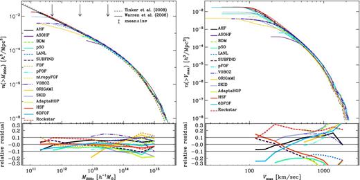
Comparison of field haloes. Upper-left panel: the cumulative mass (M200c) function. The arrows indicate the 50 particle limit for the 10243 (left), 5123 (middle) and 2563 (right) simulation data. The thin black lines crossing the whole plot correspond to the mass function as determined by Warren et al. (2006, solid) and Tinker et al. (2008, dashed). The error bars represent the mean mass function of the codes (±1σ). Lower-left panel: the fractional difference of the mean and code halo mass functions. Upper-right panel: cumulative number count of haloes above the indicated Vmax value. Lower-right panel: the relative offset from the mean of the cumulative count. The pair of solid lines in each of the residual plots simply indicates the 10 per cent error bars. Note that both properties (i.e. mass and Vmax) have been determined individually by each code.
We find that the scatter in mass is at the 10 per cent level and actually within the limits given by the two analytical functions. This scatter is driven by a variety of sources and is due to the different choices made by the finders. In particular, the finders differ on whether or not they include the mass of any substructures in the halo mass, whether or not they do unbinding and the precise definition of both the outer edge and halo centre. We note that the differences in Vmax are – in the case that each code uses its own method to determine Rmax and Vmax – substantially larger than we shall see later and of the order of 20-30 per cent.
This level of accuracy may be perfectly acceptable for some measurements, and indeed within any particular code where the assumptions employed are conserved, convergence would be expected at a much higher level. However, these errors should be indicative of the level of accuracy at which we can absolutely measure the cumulative halo mass function within a cosmological model given that, as we stressed earlier, all of the range of assumptions adopted here are perfectly physically acceptable and it is difficult to argue that one set is any better than another.
4.2 Subhaloes
For the rest of this section, we will employ a more challenging and realistic data set to answer the question: how well could we expect to do if we force the finders to use a common set of definitions? The Aquarius simulations (Springel et al. 2008) are a set of MW-sized haloes studied at a range of resolutions. We have processed the A-4 data set using a wide range of substructure finders and compared the results in Onions et al. (2012). This is a more difficult problem as now a single host halo contains several thousand subhaloes and it is the properties of these we wish to compare. Using the same ordering of panels as for Fig. 1, we show in Fig. 2 the subhaloes’ mass M200c and Vmax functions. In contrast to the field halo comparison, the mass and Vmax were calculated using a common post-processing pipeline, i.e. only the candidate identification, particle collection and unbinding procedure were different (cf. Section 2). For more details about this pipeline and the way to calculate M200c and Vmax, we refer the reader to section 4.1 of Onions et al. (2012) where also the choice of using M500c is discussed.
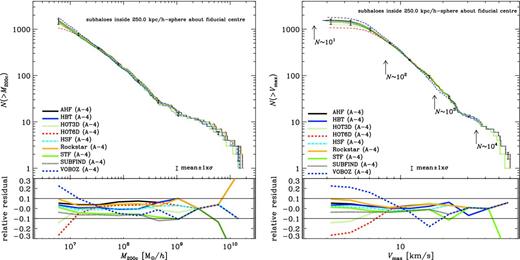
Comparison of subhaloes. Cumulative mass M200c (upper left) and Vmax (upper right) functions for the subhaloes on Level 4 of the Aquarius host A (Springel et al. 2008). The arrows in the Vmax function indicate the number of particles interior to Rmax, the position of the peak of the rotation curve. The error bars represent the mean mass and Vmax function, respectively, of the codes (±1σ). Lower-left panel: the fractional difference of the mean and code subhalo mass functions. Lower-right panel: the relative offset from the mean of the cumulative count. The pair of solid lines in each of the residual plots simply indicates the 10 per cent error bars. Note that both properties (i.e. mass and Vmax) have been determined by a common post-processing pipeline.
We find that for this more complex problem, a successful implementation of unbinding is essential in order to obtain reliable number counts anywhere near the resolution threshold. Note that the two finders adaptahop and mendieta do not feature a (reliable) unbinding procedure: adaptahop (without any unbinding) finds far too many small objects; mendieta does not contain a reliable unbinding procedure and hence finds too few objects across a large range in mass. If we were to use a common unbinding scheme for both their pre-unbinding data sets, their results would then agree with the majority of the finders. For these reasons, we drop both adaptahop and mendieta results from the rest of this discussion.
Neglecting the results from these two finders, we see in Fig. 2 that the scatter for the cumulative mass function is roughly similar to the field halo case studied in Fig. 1 despite the fact we are now using a common post-processing routine. However, the scatter in the Vmax function is considerably less than in Fig. 1 (for subhaloes composed of more than 100 particles). Both of these results are to be expected: the mass of a subhalo is sensitive to both the particle collection scheme and the unbinding procedure whereas the maximum circular velocity is less sensitive to these assumptions as this quantity only depends on a small fraction of the most central particles.
However, one may raise the issue that differences in the scatter can be due to either moving from field to subhaloes or the fact that the processing of the particles has been outsourced. To shed some more light into this, we also calculated the subhalo mass function (i.e. left-hand panel of Fig. 2) for the values directly returned by the respective code (not shown here though): we found that the differences are minuscule and hence the scatter – at least in mass – is not driven by the implementation to calculate it. As Vmax values have not been returned by the finders themselves, we are unfortunately unable to draw any conclusions about the reduction in scatter seen in the right-hand panels of Figs 1 and 2 due to our common post-processing.
Further, for subhaloes, which can be significantly tidally stripped, it is not guaranteed that the mass profile reaches the peak of the velocity curve. That is, the subhalo's radius can be smaller than Rmax. Can we hence trust the Vmax values presented here? First, this will affect all subhaloes for all finders equally due to our common post-processing. Secondly, we actually checked the ratio Rmax/R and found it to never exceed 0.5, i.e. Rmax is always substantially smaller than the subhalo's radius. However, we also acknowledge that our Rmax (and Vmax) values are based upon a single snapshot analysis at redshift z = 0, i.e. after a subhalo entered the influence of its host and experienced tidal stripping; therefore, the values reported here are solely based upon the present mass profile of the subhalo and do not necessarily reflect the original ones prior to infall.
We would like to close with a cautionary remark about the relative residual curves presented in the lower panels of Figs 1 and 2: these ratios are actually measuring the difference in the number of objects found by a certain halo finder above a given mass or Vmax threshold, respectively. They do not directly measure the differences in mass or Vmax. In that regard, there are two errors entering into these residuals: variations in the number of identified haloes (above a threshold) and differences in the recovered mass of the same object between finders. The following subsection will now focus on the latter effect, quantifying the scatter across finders for the same object.
4.2.1 A common set of objects
Before quantifying the actual deviations between various properties, we want to define a set of objects that could be used for this purpose. Note that distribution functions will not only suffer from differences in individual halo properties but also encode the fact that some finders may have identified different numbers of objects. To circumvent this, we aim at directly comparing quantities on a halo-to-halo basis and move on from general distribution functions and their variations as discussed above.
To cross-identify objects, we use a halo matching technique that correlates all haloes found by a given halo finder to the catalogue of another finder by examining the particle ID lists and maximizing the merit function |$C=N_{\rm shared}^2/(N_{1}N_{2})$|, where Nshared is the number of particles shared by two objects, and N1 and N2 are the number of particles in each object, respectively (see e.g. Klimentowski et al. 2010; Libeskind et al. 2010 for more details, as well as Appendix B for different merit functions). By restricting ourselves to the set of objects found by every halo finder, we are able to directly compare the properties of the same object across all finders. We will discuss the excess objects in Section 5.1.1 and caution reader that this common set can be dictated by one finder not finding a sufficient number of haloes in the first place.
Please note that for this analysis we also only used the ‘Subhaloes going Notts data set; this project featured a common post-processing pipeline based upon individual particle ID lists. These lists make subhalo cross-matching as outlined above feasible. In order to avoid any possible ambiguities with the exact definition of position, bulk velocity, mass and Vmax calculation implemented by every algorithm, participants were asked to return only the lists of those particles that they consider bound/belonging to each object; the centre, bulk velocity, edge/mass, as well as various derived quantities were then calculated by a common post-processing pipeline, i.e. positions are iteratively determined centre of masses using the innermost 50 per cent of particles, the bulk velocity is the mean velocity of all particles, the mass corresponds to M200c (as defined by equation 2 when applying Δref = 200 and ρref = ρcrit), Vmax is the peak value of the rotation curve, the shape is the ratio between the smallest and largest eigenvalues of the moment of inertia tensor |$\mathcal {M}_{jk}$| (cf. equation 7) and the spin parameter λB as given in equation (4). This approach and the use of a common data set, which might be biased towards rather clean subhaloes that are easier to detect, mean that the scatter reported here should be considered lower limits.
The plots in Subsections 4.2.2 through to 4.2.5 now all follow the scheme: the x-axis shows the median of the subhalo mass med(M) whereas the y-axis gives the normalized difference between the lower and upper percentiles equivalent to the third and seventh ranked of the distribution across all nine (sub)halo finders. We deliberately chose to use medians and percentiles as the distribution of properties across finders is highly non-Gaussian and at times biased by just one or two outliers. The plots further show medians in four mass bins as histograms to highlight any possible dependence on mass. And those points for which the difference between the third and seventh percentiles is zero are shown at the bottom of the y-axis. The number of cross-matched subhaloes is 823 and should be compared against the total number of objects found by each individual (sub)halo finder given in table 2 of Onions et al. (2012, Aq-A-4 row); however, for convenience we list here in Table 3 the number of subhaloes found by each code in excess of the common 823 objects. Fig. 8 indicates that the majority of these missing objects are small, containing less than 200 particles.
Total number of subhaloes and the ones found in excess of the common set of 823 objects of the Aquarius A-4 data set. All subhaloes are requested to contain 20 or more particles and have their centres within a sphere of radius 250 h−1 kpc from the fiducial centre. Fig. 8 indicates that the majority of these missing objects are small, containing less than 200 particles.
| Code | Total number of objects | ‘Excess’ objects |
|---|---|---|
| ahf | 1599 | 776 |
| hbt | 1544 | 721 |
| hot3d | 1265 | 442 |
| hot6d | 1075 | 252 |
| hsf | 1544 | 721 |
| rockstar | 1707 | 884 |
| stf | 1521 | 698 |
| subfind | 1433 | 610 |
| voboz | 1863 | 1040 |
| Code | Total number of objects | ‘Excess’ objects |
|---|---|---|
| ahf | 1599 | 776 |
| hbt | 1544 | 721 |
| hot3d | 1265 | 442 |
| hot6d | 1075 | 252 |
| hsf | 1544 | 721 |
| rockstar | 1707 | 884 |
| stf | 1521 | 698 |
| subfind | 1433 | 610 |
| voboz | 1863 | 1040 |
4.2.2 Position and bulk velocity
In Fig. 3, we start by inspecting the errors in position and velocity with the former deviation Δpos normalized by the median radius for the object, med(R), and the latter Δvel by the median of the peak of the object's rotation curve, med(Vmax). We can see a trend for both variations to decrease for more massive objects (especially for the position), but the errors are rarely larger than a few per cent with the overall median error being 0.2 and 0.8 per cent for position and velocity, respectively. The trend with mass reflects the resolution dependence of the accuracy of both the position and bulk velocity of the (sub)haloes. This scatter is consistent with that observed in Knebe et al. (2011a) for mock haloes.
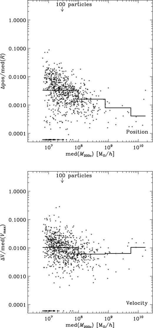
Relative errors in the recovered positions (top) and velocities (bottom) of the subhaloes found by all finders. The errors are scaled by the median size of the object and the median Vmax, respectively.
4.2.3 Mass
The recovery of subhalo mass is presented in Fig. 4. We no longer see a prominent trend with mass anymore. The discrete nature of the particle masses is evident; the difference ΔM (again normalized by the median of the mass itself) can only be a multiple of the actual particle mass which gives rise to the diagonal stripes visible in the plot for lower mass objects. The overall median of the scatter is found to be 3 per cent.
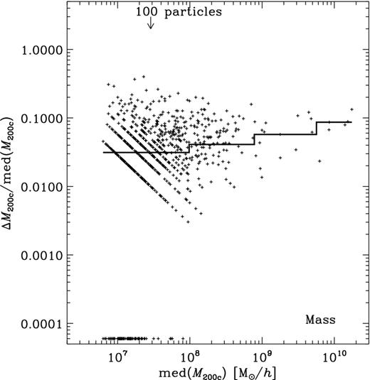
Relative errors in the recovered mass for the subhaloes found by all the finders. The errors for each object are scaled by the median mass found for the object.
4.2.4 Vmax and Rmax
Let us consider next the magnitude and radial location of the peak in the rotation curve of the halo, characterized by the values of Rmax and Vmax, respectively. It has been claimed that these quantities provide a good proxy for the mass and spatial scale of the object (see e.g. Ascasibar & Gottlöber 2008; Muldrew, Pearce & Power 2011), and our previous comparisons (Knebe et al. 2011a; Onions et al. 2012) show that this may indeed be the case, especially for the maximum circular velocity. We can indeed see in Fig. 5 that the scatter in the Vmax value (normalized to Vmax itself) is lower than for the mass having a median of a mere 0.6 per cent. However, the variations in Rmax are naturally larger due to the uncertainty in the determination of the peak position: the rotation curves show a flat behaviour about Rmax leading to a median error of 2 per cent.
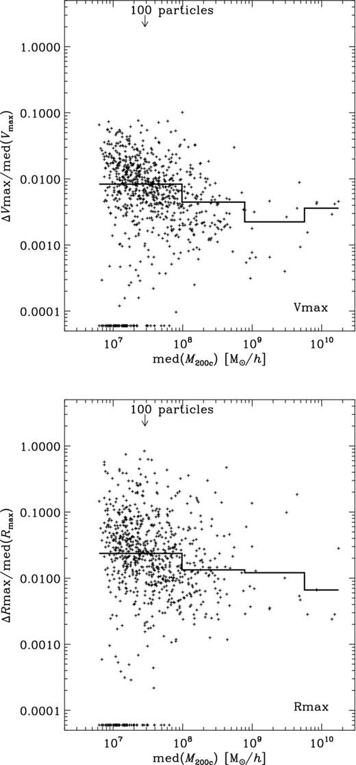
Relative error in Vmax (top) and Rmax (bottom).
4.2.5 Shape and spin
In Fig. 6, we will now turn our attention towards the shape and spin of the objects identified by the halo finders. The calculation of these quantities is more involved and hence we expect the scatter to be larger, e.g. several of the errors already reported here will propagate in a non-linear fashion to these properties. While the shape [defined here as sphericity, i.e. the ratio between the smallest and largest eigenvalues of the moment of inertia tensor defined by equation (7)] appears to be determined to approximately the same order of magnitude as the previous quantities giving a median of 5 per cent, the spin is less precisely determined with a median of 18 per cent. For a more elaborate discussion of the spin using the same data and finders as presented here, we like to refer the reader to Onions et al. (2013).
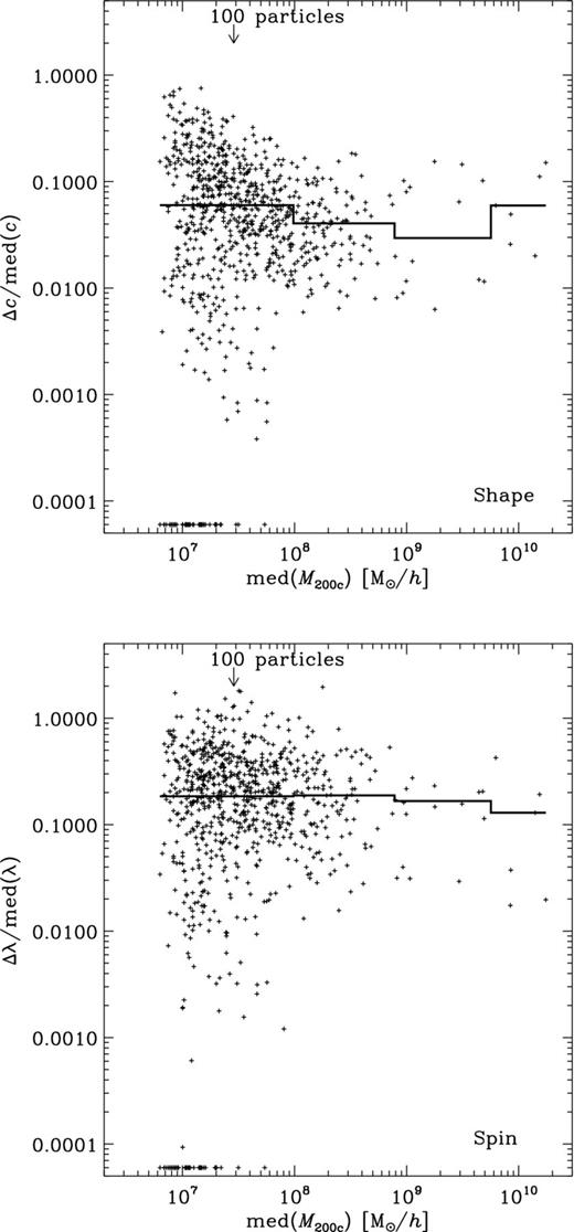
Relative errors in shape (top) defined as the ratio between the smallest and largest eigenvalues of the moment of inertia tensor defined by equation (7) and spin parameter λB (bottom).
4.3 Galaxies
In Knebe et al. (2013), we presented a comparison of codes as applied to the Constrained Local UniversE Simulation (CLUES) of the formation of the Local Group which incorporates much of the physics relevant for galaxy formation. We compared both the properties of the three main galaxies in the simulation (representing the MW, Andromeda and M33) and their satellite populations for a variety of halo finders ranging from phase space to velocity space to SO-based codes, including also a new mere baryonic object finder. We obtain agreement amongst codes comparable to our previous comparisons – at least for the total, dark and stellar components of the objects. However, the diffuse gas content of the haloes shows great disparity, especially for low-mass satellite galaxies. This is primarily due to differences in the treatment of the thermal energy during the unbinding procedure. We acknowledge that the handling of gas in halo finders is something that needs to be dealt with carefully, and the precise treatment may depend sensitively upon the scientific problem being studied.
To give an impression of the differences found, we extracted all the particles from the simulation data in a spherical region about the centre of a certain subhalo. The results can be viewed in Fig. 7. We can clearly see that the region about the object's centre contains a substantial number of gas particles (shown in the upper-left panel). All codes featuring a treatment of the gas thermal energy either during or prior to the unbinding (i.e. ahf and subfind) remove essentially all gas from the subhalo; whereas rockstar, which does not include the thermal energy during the unbinding, and stf, which does not process the gas and stars through an unbinding routine, are left with a residual amount of gas. Note that jump-d is designed to find galaxies and ignores the DM.
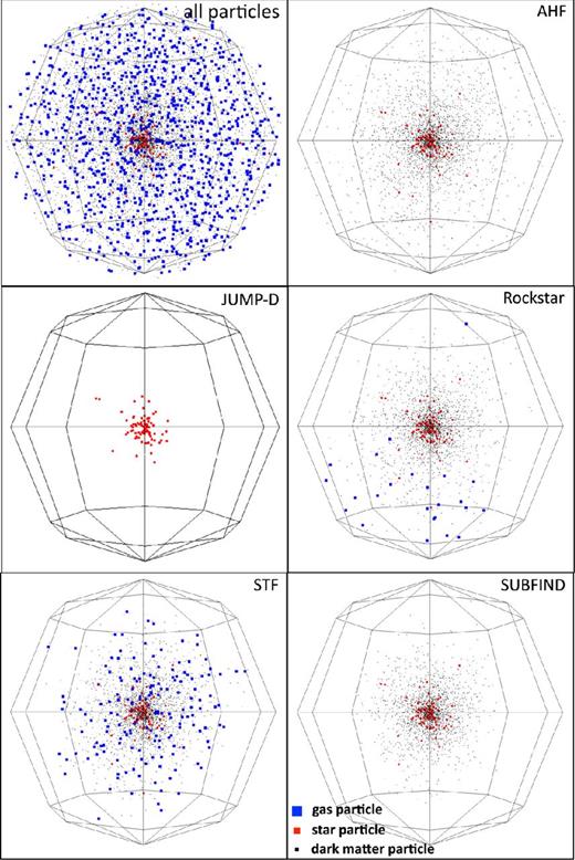
Visualization of a subhalo showing all particles inside a spherical region about the identified centre (upper-left panel) versus the actually identified particles of the individual halo finder showing all types of particles: gas (blue), stars (red) and DM (black).
When using ahf in a mode where the gas thermal energy has been ignored, ahf basically considers all gas particles seen in the left-hand panel to be part of the subhalo. In contrast, due to their phase-/velocity-space nature, both rockstar and stf consider the majority of the gas particles to belong to the background host and keep only a small amount of them. For the object considered here, the effective thermal velocity of each gas particle is always larger than its kinetic velocity (not shown here) and hence the grouping in phase or velocity space will naturally remove (hot) gas whenever a gas particle is considered not belonging to it based upon kinetic velocity only. Or put differently, the gas component forming part of the background halo is prone to be removed by such finders as they inherently use velocity information when grouping and collecting the initial set of particles, whereas configuration-space finders only deal with velocities (either kinetic or thermal) in a (post-processing) unbinding procedure. On a side note, a visual inspection of a larger region about this particular sample satellite galaxy indicates that it has passed extremely close to its host already and been subjected to severe tidal forces; this might also explain why rockstar associates gas with one side of the galaxy.
4.4 Summary
There are several sources of uncertainty in the properties computed by halo finders. While Section 3 was concerned with the ambiguities arising from the definition of each quantity, here we have also quantified the scatter due to the different procedures followed by each halo finder in order to compute the same quantities from the same data. Our results are succinctly summarized in Table 4. While the differences are below 1 per cent for position, bulk velocity and Vmax (and still marginal for masses), they can rise to over 15 per cent for certain derived quantities such as the spin parameter. Without any further investigations, these numbers could in fact indicate reasonable error bars to be attached to any study based upon the results derived from a single halo finder. However, the values listed in Table 4 should be considered lower limits as we have restricted the comparison to objects found by all halo finders and used a common post-processing pipeline.
Scatter in the main properties computed by the halo finders. Note that this error is only a lower limit, especially for the numbers based upon the set of common objects.
| Quantity | Scatter |
|---|---|
| Set of common objects: | |
| Position | <1 per cent R200 |
| Bulk velocity | <1 per cent Vmax |
| M200c | 3 per cent |
| Vmax | <1 per cent |
| Rmax | 2 per cent |
| Shape | 5 per cent |
| Spin | 18 per cent |
| Full catalogues: | |
| Mass function | 10 per cent |
| Vmax function | 20-30 per cent |
However, this is a rather academic situation as in reality neither are the objects found by each halo finder restricted to some common set nor will the properties be calculated applying the same method or definition or even common post-processing pipeline. To this extent, we also presented the scatter in the general mass and Vmax functions noting that it is in fact larger than the lower limits derived before. But what is responsible for this scatter? Are there ways to understand its origin and hence possible post-correct for it? The sources of the scatter are certainly two-fold, i.e. the individual particle collection and unbinding procedures of each finder. Different finders do not necessarily find the same set of objects, and they retrieve variations in the properties of the same object. We explore these possibilities in more detail in the next section and discuss the relevance of this variation for scientific applications in Section 6.
5 PRECISION COSMOLOGY?
One of the most pressing questions arising from the plots presented in the previous section is: ‘Why is there a residual scatter between halo finders of up to 10 per cent?’ The finders have been applied to the same data, subjected to a common post-processing pipeline, and, in some cases, even compared on a set of objects identified in common. As mentioned before, unless we can be certain which halo-finding technique is the best (if such a statement can be made at all), the observed scatter indicates the accuracy to which we can determine these properties in cosmological simulations. In this section, we will try to pinpoint the origin of the observed scatter by examining the contribution of the different steps outlined in Section 2. Our final goal is to see if it is possible to bring the errors incurred by halo finding down to the 1 per cent level demanded by precision cosmology (e.g. Tinker et al. 2008; Komatsu et al. 2011).
5.1 Origin of the scatter
What are possible sources for the observed scatter? We have already seen that there are two fundamental steps involved in obtaining halo catalogues, i.e.
In that regard, the differences seen in Fig. 1 combine uncertainties in both these steps whereas Fig. 2 is only subjected to the first point thanks to the common post-processing pipeline. For the time being we will actually leave the investigation of differences due to the second point aside and only focus on the mode of operation of halo finders. But one also has to go one step further and ask whether one is interested in the actual halo-to-halo scatter or systematic errors affecting the whole halo ensemble. This is an important point as we have seen that the variations in, for instance, the halo mass for cross-identified objects are of the order of 3 per cent (cf. Table 4), whereas the ensemble mass function of the same data set seen in Fig. 2 clearly shows larger scatter: while the number of uniquely found haloes is 823, each finder nevertheless found approximately the same number of objects not part of the common pool (cf. Table 3). This suggests that once the halo finders do find the same set of objects, the errors across them should decrease approaching the first set of values listed in Table 4. As we have shown, most of the missing objects are small. Hence, one way to improve the ‘purity’ of a catalogue is to only rely on objects containing more than 300 particles. This should not be too surprising as this is the same limit found elsewhere (e.g. Onions et al. 2013) to be required if stable derived halo properties (such as the spin parameter) are desired.
Focusing on the halo finder methodology and following the scheme of Section 2, all the differences between one halo finder and another must fall into one of the following categories, representing the basic steps required to end up with a halo catalogue:
candidate identification;
halo centre and bulk velocity determination;
particle collection and unbinding procedure;
mass and edge determination.
We will now follow a divide-and-conquer strategy, in an attempt to isolate those steps that are responsible for most of the scatter, again using the Aquarius A, Level 4 data set and restricting ourselves to the commonly post-processed particle ID lists of some of the finders featuring a credible unbinding procedure. While we include mass and edge determination in this list, we do not discuss it below as with a common post-processing pipeline this step is the same for all finders and introduces no scatter. This highlights the issue mentioned above that in actuality a common post-processing routine is not used by everybody and significant scatter can be introduced at this stage unless great care is taken.
5.1.1 Candidate identification and ‘excess’ objects
There is one element that could make a sizeable contribution to the scatter in the mass and Vmax functions: whether a given halo is detected or not. Remember that the deviations reported in Table 4 were based upon a common set of objects, but that each finder certainly found (substantially) more objects than defined by this common set (cf. Table 3). For every subhalo found by a given reference code in the Aquarius A-4 data, we now identify its counterpart in the particle ID lists of all other codes. This was again accomplished by examining the particle lists and maximizing the merit function |$C=N_{\rm shared}^2/(N_{1}N_{2})$|, where Nshared is the number of particles shared by two objects, and N1 and N2 are the number of particles in each object, respectively (see Appendix B for more details). This is the same procedure as applied before, but this time we aim at quantifying how many of the objects found by a given halo finder were found by the other finders.
To investigate this, we plot in (the upper panel of) Fig. 8 the fraction of codes that also found the same object on the y-axis against the (binned) number of particles of the object in the reference code. We can see that there is a group of codes for which all other codes found the same objects (with also approximately the same number of particles). In the lower panel of Fig. 8, we show the actual number of objects entering into the histograms of the upper panel, i.e. the number of haloes found by each finder in the respective number of particle bin.
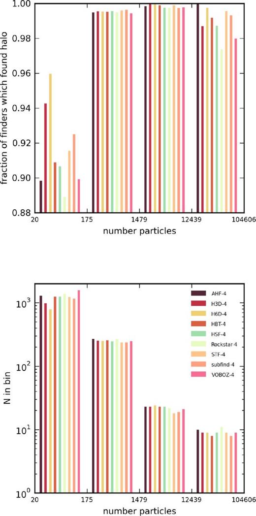
The fraction of codes finding the same object as the reference code given in the legend as a function of the binned object's number of particles in that reference code (upper panel) as well as the actual number of objects entering the comparison in the respective number of particle bin (lower panel).
While there are differences visible in Fig. 8, how will they affect, for instance, the (sub)halo mass or Vmax function – our usual measure for the scatter? This can be viewed in Figs 9 and 10, where we show (in the upper panel) the subhalo mass function and the Vmax function, respectively. The three sets of lines in each panel refer to the original functions based upon all objects found by each finder (shifted upwards by a factor of 2 for clarity; cf. Fig. 2) and the same function using only the set of common objects (middle lines, shifted downwards by a factor of 2 for clarity) as well as the ‘excess’ objects (lower lines, also shifted downwards by a factor of 2) as defined in Section 4.2.1. The three lower panels in each of the figures show the fractional difference of the curve for a given finder to the mean value. Remember that these curves quantify the variation in the number of objects found above a certain mass threshold; they do not directly measure differences in subhalo mass. We see here that restricting ourselves to the common set does not change the observed scatter in the mass function, whereas we find a marginal improvement for Vmax. Note that the perfect agreement of the functions for the common set at the imposed 20 particle limit is artificial as the number of objects is identical by construction. And even though we clearly observe that the scatter for the excess objects is substantially larger than for the common ones, these results indicate that the overall scatter is not dominated by them. These objects contribute particularly at the low-mass end where their consistent detection becomes difficult, but variations in subhalo properties from code to code are principal source here. We finally note that the excess subhaloes are primarily of low mass and composed of less than 100 particles. One last word of caution, the error estimates presented in Subsections 4.2.2 through to 4.2.5 (and summarized in Table 4) are smaller than the scatter seen here as they only took into account the difference in the third and seventh percentiles and hence ignoring outliers seen here.
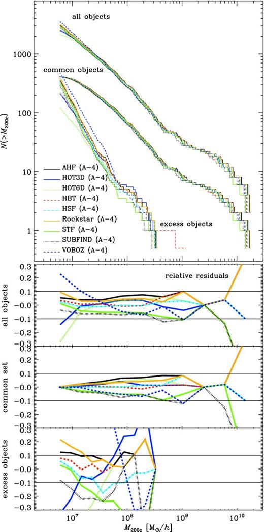
Subhalo mass M200c functions for all identified objects (upper set of lines), the common set of objects (middle lines) and the excess objects (lower lines). The lines for all objects have been shifted upwards by a factor of 5 whereas the other two sets have been shifted downwards by a factor of 5 for clarity. The lower three panels show the relative residuals with respect to the mean (as in the plots before), and the pair of solid lines in each of them indicates the 10 per cent error bars.
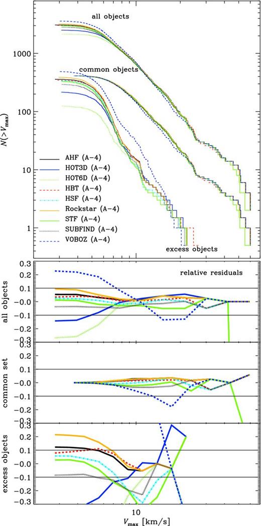
We have seen before that halo finders perform differently at finding subhaloes close to the centre of their host (Knebe et al. 2011a; Muldrew et al. 2011; Onions et al. 2012). This then raises the question whether or not this is the origin for the existence of the excess objects seen here. We therefore present in Fig. 11 the cumulative radial distribution of these objects (normalized to the respective total number of excess haloes) always in comparison to the full set of haloes; both curves have been shifted by a factor of 5 for clarity as they would otherwise overlap at the low-r end of the distribution. We can appreciate that excess subhaloes are found at all possible radial distances. And it comes as no surprise that those objects found close to the host centre are forming part of the excess set. We recommend to view the radial distance plot in relation to fig. 7 of Onions et al. (2012) that shows the cumulative mass in subhaloes as a function of distance.
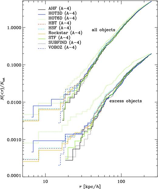
Subhalo radial distance functions for all identified objects (upper set of lines) and the ‘excess’ haloes (lower lines). In each case, the upper and lower curves have been scaled by a factor of 5 to better separate them.
5.1.2 Centre and bulk velocity determination
Given that we found a fair agreement for (sub)halo centres in (the upper panel of) Fig. 3, and that there is little difference between Fig. 1 (no common post-processing) and Fig. 2 (common post-processing), it seems unlikely that the details of the location of the centre or the calculation of the bulk velocity of an object make a significant contribution to the error budget. But we nevertheless performed the following tests for which the results regarding the Vmax function are presented in Fig. 12: using one of the halo finders only we varied the definition of the centre as used with our common post-processing pipeline assessing the effect it has on both the mass and Vmax. The definitions applied were the overall centre of mass, the position of the most bound particle and an iteratively determined centre using the innermost 10 or 50 per cent of the particles. We found that while the mass is not affected at all (variations below 1 per cent), Vmax can change up to several per cent for certain subhaloes. These results are also in agreement with the findings reported for the mock haloes studied in Knebe et al. (2011a). We therefore rather conjecture that either the particle collection method or the particulars of the unbinding procedure may be held responsible for the scatter, both to be studied in the following subsection.
Subhalo Vmax function to various definitions of subhalo centre. Please refer to the main text for more details.
5.1.3 Particle collection and unbinding
Obviously, one cannot come up with either a unique candidate identification or particle collection method, as these clearly define the halo finder in question: for instance, phase-space finders base their particle collection on an intrinsically different algorithm than configuration-space finders, and fof-based methods usually combine these two steps into one single procedure – and they may also not apply any (additional) edge definition other than the isodensity contour traced by the applied linking length. Unbinding is also an important – and delicate – step, and the particular way of carrying it out may be regarded as an intrinsic piece of some algorithms.
For the Aquarius A-4 data set, we now separate the two steps of collecting particles and removing unbound particles from each other and show in Fig. 13 the resulting subhalo mass functions (upper inset panels) and the resulting variations (lower inset panels). The top plot shows the subhalo masses as given right after the collection of particles considered potentially belonging to an object by each finder, whereas the bottom plot takes those subhaloes and subjects them to a common unbinding procedure.6 Please note that not all halo finders participated in this particular test. While there are huge differences in the amount of particles that each algorithm chooses to evaluate for (un)binding, applying a common procedure to all those candidate objects reduces the scatter to the level already seen in Fig. 2, where the unbinding was left to the individual halo finders. On a separate note, this figure also clearly indicates how important unbinding is for configuration-space finders versus phase-space finders. The mass function for configuration finders such as ahf, mendieta, VOronoi BOund Zones (voboz) and subfind changes significantly after unbinding whereas the distributions for hot6d, rockstar and stf do not.
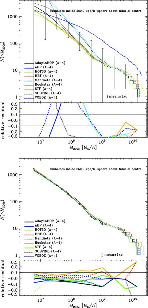
Highlighting the relevance of a common unbinding procedure: we show the same subhalo mass function as in Fig. 2, computed from raw particle lists returned by each code without unbinding (top panel) and with a common post-processing routine that also features a common unbinding procedure (bottom panel). The pair of solid lines in each of the residual plots simply indicates the 10 per cent error bars.
To quantify the influence of unbinding even more, we performed yet another test: we requested participating halo finders to provide the escape velocity profile for a given pre-selected (massive) subhalo originally found across all analyses. The results are presented in the left-hand panel of Fig. 14, where we plot the calculated escape velocity |$v_{\rm esc}=\sqrt{2|\phi |}$| at each particle position, normalized by the average over the four partaking codes. First, one can see that different codes do in fact use different methods to calculate the gravitational potential and hence escape velocities. This is particularly the case for ahf, which uses a spherical approximation when calculating the potential ϕ, whereas the other three codes base their ϕ value on a tree construction of the particles. The spikes (dips) in the profile are sub-substructure objects that are not resolved by the (non-realistic) spherical method applied in ahf. The right-hand panel shows escape velocity profiles after unbinding. The differences have marginally increased for the tree-based potential calculation, reflecting again the particulars of the individual unbinding procedures, such as what velocity is used to determine whether a particle is (un)bound. The few per cent uncertainty in the escape velocity of the individual particles eventually leads to a 0.5 per cent error in the different masses after unbinding here. Consequently, unbinding is unlikely to be a primary source of the scatter observed (see also Table 4).
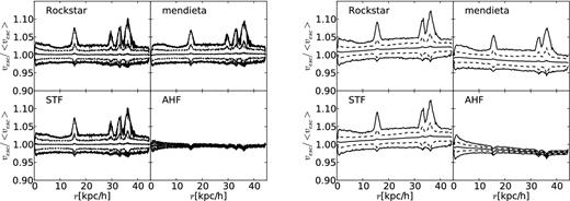
Escape velocity profile for a sample (massive) subhalo as determined by a sample of the halo finders prior to their unbinding procedure (left-hand panel) and after individual unbinding (right-hand panel). The lines indicate the mean (solid), mean ±1σ (dashed) and minimum as well as maximum value (solid) in the respective bin for each finder normalized by the binned means of all finders.
Before we continue, we should emphasize that the term ‘unbinding’ is a little misleading. First, these structures do not exist in isolation but are treated as such when determining the binding energy. A particle near the edge might be considered bound if an object is treated in isolation but could be stripped by tidal forces. Secondly, a reference frame must be chosen to determine the kinetic energy of a particle. Some codes may choose to use an object's bulk velocity, others may use the velocity of the density peak, and other may use the velocity of the particle residing at the minimum of the gravitational potential. All of these are valid choices. Thirdly, all so-called unbinding procedures use the instantaneous energy of a particle. Though particles that are false positives with high relative velocities are unlikely to remain with a subhalo, particles that are deemed to be marginally unbound might only be tidally stripped on time-scales approaching a dynamical time. Only particles that leave the phase-space volume of a subhalo on time-scales much shorter than a dynamical time can truly be said to be unbound. However, such a criterion is rarely considered when determining the ‘bound’ mass of a subhalo.
Despite these complications, we have to acknowledge that even with a common unbinding procedure there still remains a significant degree of scatter. This is not surprising given the large differences in the set of collected particles (i.e. upper panel of Fig. 13). We conclude that errors in the subhalo mass of the order of 10 per cent result from the different initial particle collection scheme intrinsic to each method.
5.2 Potential improvements: facilitating merger trees
As already touched upon in Section 2.6, it is often the case that we not only have the end-state of a particular simulation but also the evolutionary history at a series of earlier times. We can then make use of this additional information to calculate the temporal evolution of haloes. It has been shown that software tracking haloes across snapshots can actually improve the results and reliability of halo finders (Springel et al. 2001b; Gill et al. 2004a; Tormen et al. 2004; Tweed et al. 2009; Behroozi et al. 2013a; Benson et al. 2012; Han et al. 2012). This is achieved by explicitly ensuring dynamical consistency of halo properties across timesteps. Note that a lot of these papers primarily deal with subhaloes and following them after infall into the host. But the publicly available tool presented by, for instance, Behroozi et al. (2013a) is applicable to both distinct haloes and subhaloes. It follows a preliminary merger tree but simultaneously integrates the movement of haloes backwards in time: knowing the positions, velocities and mass profiles of haloes at one timestep, one may use the laws of gravity and inertia to predict their properties at adjacent timesteps. This allows the removal of spuriously defined objects or for the insertion of objects not properly identified by the halo finder in the first place. The method employed by Behroozi et al. (2013a) improves the completeness of the halo catalogues in general, particularly at earlier redshifts, even though the results obviously depend on the completeness of the catalogue used as the initial input (generally the z = 0 snapshot analysis). For more elaborate details, we refer the interested reader to the aforementioned paper.
Such merger trees are now routinely used as inputs to semi-analytic models of galaxy formation to provide the backbone within which galaxy formation takes place (e.g. Cole et al. 2000; Benson et al. 2002; Bower et al. 2006; Croton et al. 2006; De Lucia et al. 2006; Bertone, De Lucia & Thomas 2007; Font et al. 2008). Therefore, Benson et al. (2012) have studied the convergence in the stellar and total baryonic masses of galaxies, distribution of merger times, stellar mass functions and star formation rates in the GALACTICUS model of galaxy formation (Benson 2012) as a function of the number of snapshots used to represent dark matter halo merger trees. They found that at least 128 snapshots are required in between redshifts z = 20 and z = 0 to achieve convergence to within 5 per cent for galaxy masses, highlighting again the importance of ‘sufficient’ temporal information for the post-processing of the halo catalogues.
Further, the utilization of DM halo merger trees entails another ‘feature’ for workers in the field of semi-analytical galaxy formation, the so-called orphan galaxies (Gao et al. 2004a): it can and does happen that a DM subhalo dissolves due to tidal forces (and lack of numerical resolution) while orbiting in its host halo (e.g. Gill et al. 2004b for a study of these disrupted subhaloes). However, a galaxy having formed prior to this disruption and residing in it should survive longer than this subhalo. Therefore, it became standard practice to keep the galaxy alive even though its subhalo has disappeared, calling it ‘orphan’ galaxy (Springel et al. 2001b; Gao et al. 2004a; Guo et al. 2010; Frenk & White 2012). This is another example of the benefits of using merger trees once the simulation of the halo finder does not provide sufficient information anymore. But we also caution the reader that the utilization of these orphan galaxies is certainly resolution dependent and should be done with care.
But in any case, such merger tree-based comparisons and improvements, respectively, are beyond the scope of the present work, but will certainly form part of the next halo finder workshop scheduled for 2014.
5.3 Summary
Primarily studying subhaloes in the Aquarius simulation, we have been able to associate some of the scatter between the halo finders with inconsistent property definitions and differences in the unbinding routines. However, the most significant part of the scatter seems to stem from the differences in the initial particle collection. Given the present situation, the best halo finders can do for precision cosmology is to provide error bars of 10 per cent on halo mass and Vmax functions of which the prime contribution comes from the initial particle collection and (to a smaller degree) subtleties in the way the unbinding is performed. Note that these two parts are intrinsic to the method of the halo finder. While one might still aim at outsourcing the unbinding, the actual collection of particles is the halo finder stripped down to its bare minimum. Making any changes here is equal to simply using another halo-finding technique.
We nevertheless need to remind the reader that the situation is a bit different for field haloes and subhaloes. For the latter, edges and detection thresholds are defined so differently among the finders that a 10 per cent mass difference after common unbinding is not inexplicable. For the former, the reasons for discrepancies are substantially reduced to issues of definition (and possibly bugs). In that regard, we can only reiterate that the end user of any halo catalogues needs to make sure to understand the mode of operation of the halo finder upon which the catalogue is based. But the good news here is that for basically all properties studied here, the error decreases with increasing number of particles in the object.
But we also need to bear in mind that there is a subtle difference between disparities in general distribution functions and variations of properties of individual objects. The aforementioned error of approximately 10 per cent may in part be driven by the fact that halo finders return different numbers of objects above a certain threshold (be that mass, Vmax, etc.), but we have shown that this effect is virtually negligible at all but the smallest masses (see the top panel of Fig. 11). This error is mostly due to the scatter in the mass assigned to each individual halo, but it is exacerbated by the steepness of the cumulative mass function. Our one-to-one comparison of halo masses (Fig. 4) finds that this scatter is substantially smaller, of the order of 3 per cent only.
There are clear indications that a more sophisticated construction of merger trees might reduce incompleteness (Behroozi et al. 2013a; Han et al. 2012), albeit that any possible biases in the initial halo catalogue upon which the revised trees will be based will remain. But the question still is, whether or not (and how) this will affect the end user of halo finders and the scientific applications across fields that require halo catalogues as an input. We shall discuss these implications in the following section.
6 ASTROPHYSICAL APPLICATIONS
The applications of (sub)halo catalogues of numerical simulations spread over various fields in astrophysics. These range from facilitating the interpretation of numerical simulations over constituting input to semi-analytic models to comparison and analysis of observational data. In this section, we comment on the different applications and the influence/relevance of the halo-finding uncertainties on the results in other fields.
6.1 Galaxy formation, semi-analytics and merger trees
We start with one of the biggest topics, i.e. the formation of galaxies within a cosmological context. There are presently two routes to this: one is to directly simulate cosmological volumes including all the relevant baryonic physics (see Scannapieco et al. 2012 for a recent comparison of various baryonic physics and methods), another is to defer to DM-only simulations and apply semi-analytical recipes to them (Cole et al. 2000; Benson et al. 2002; Bower et al. 2006; Croton et al. 2006; De Lucia et al. 2006; Bertone et al. 2007; Font et al. 2008). And the latter is in fact one of the major areas that require well-understood and carefully constructed halo catalogues.
6.1.1 Semi-analytical galaxy formation
Modern semi-analytical codes (Croton et al. 2006; Monaco, Fontanot & Taffoni 2007; Somerville et al. 2008; Henriques et al. 2009; Benson 2012) usually take as input halo merger trees derived from large numerical simulations rather than purely analytical forms such as Press & Schechter (1974) or extended Press–Schechter (Bond et al. 1991). Stable semi-analytic models require stable and physically realistic merger trees: haloes should not dramatically change in mass, size or jump in physical location from one step to the next. As we have seen above, all of these changes can result from a poorly constrained halo finder, with halo size being particularly ill-determined. If care is not taken with the choice of the halo centre, this can move dramatically from one step to the next, particularly during a large merger event. This dynamical process also leads to large-scale bridging between structures during the initial particle collection phase. This can lead to substantial changes in an object mass in a very short time-scale. Such changes are unphysical. Great care also needs to be taken to construct a clean halo catalogue from which to build the trees. The primary concern here is that only gravitationally bound structures are used; otherwise, particularly in regions adjacent to large objects where the background density is already enhanced, spurious groupings can be claimed. Thus, we recommend that only halo-finding algorithms with a well-tested unbinding stage should be used to create catalogues that are intended to form the basis of a semi-analytic model.
Subhalo tracking is also sometimes incorporated into semi-analytic models. We caution that care should be taken with this approach as some algorithms (e.g. subfind) are very conservative in their allocation of mass to substructures. In this case, the subhalo mass can drop dramatically as the structure moves closer to the centre of a host, occasionally vanishing entirely only for it to be partially recovered again afterwards (see, for instance, figs 10–12 of Knebe et al. 2011a or figs 4 and 5 of Muldrew et al. 2011). While all tested finders do a good job of actually locating substructures, even close to the very centre of the host halo, the recovered subhalo mass as a function of the distance to the host halo centre is a function of the particular halo finder we are using (Knebe et al. 2011a; Muldrew et al. 2011).
This effect certainly influences the so-called orphan galaxies (cf. Section 5.2), that is galaxies that are no longer associated with a DM subhalo. How these galaxies are treated varies from model to model and also depends on the resolution of the underlying simulation. The most common approach is to associate the galaxy with the most bound DM particle at the snapshot just before the subhalo has vanished from the halo catalogue. Subsequently, either this particle is tracked or an orbit is estimated based on the properties of this particle and the galaxy is allowed to survive for a merging time computed using the Chandrasekar formula (e.g. Gao et al. 2004a; Guo et al. 2011). None of the current semi-analytical codes account for the possibility that the subhalo will ‘reappear’ at a later time. However, some codes producing merger trees do attempt to correct for this artificial subhalo removal (Behroozi et al. 2013a; Han et al. 2012). The effect this correction will have on the galaxy population produced by semi-analytic models will certainly be one of the hot topics discussed at future workshops.
A related issue is that of major merger events. As soon as two nearly equal mass haloes approach each other and their radii start to overlap, how will halo finders deal with this? Some codes (e.g. ahf) have the intrinsic problem that one of them will be tagged ‘host’ and the other ‘subhalo’ at some stage of the merger; this will then evidently lead to a misassignment of mass. For a more elaborate study and discussion of this effect, we refer the reader to Behroozi et al. (in preparation).
Another important input to semi-analytical models is the spin parameter of DM haloes as the size of the galactic disc residing within them is often derived from this parameter, via i.e. conservation of angular momentum leading to the formation of a rotationally supported disc (e.g. Mo, Mao & White 1998). Some models assume a simple relation between a disc size and the spin parameter and use a fiducial value for the spin parameter, often derived from simulations (Lu et al. 2011). Others use the current angular momentum or spin parameter of the host halo to determine the angular momentum of the disc (e.g. Guo et al. 2011; Benson 2012) and these codes require this information to be present in the halo merger tree. However, the spin is the least faithfully recovered quantity amongst different halo finders (e.g. Section 4) as it is the most sensitive to the unbinding procedure. In fact, Onions et al. (2013) showed that the spin parameter can be used as a metric to determine how well a (sub)halo finder prunes its particle collection of high-velocity interlopers. The impact of an unstable or poorly measured spin parameter is likely small given the uncertainty in the baryonic physics used in semi-analytical modelling to convert a halo spin to the spin of a gas and stellar disc. However, given its use as a metric for assessing the quality of a halo catalogue and its use as a diagnostic for identifying unrelaxed (read merging) haloes (e.g. Klypin, Trujillo-Gomez & Primack 2011), it warrants further investigation before its default inclusion in halo merger tree construction.
One quantity commonly derived with semi-analytical modelling is the luminosity of the galaxy residing within the DM (sub)halo identified by the object finder. And typically observational luminosity functions are better constrained than mass functions that consist of derived quantities. However, comparisons with luminosity functions from numerical simulations are not only challenging because of the differences between various (sub)halo finders: currently, the variety of subgrid models in hydrodynamical simulations of galaxy formation introduces significantly larger uncertainties (Scannapieco et al. 2012), and the same is true for semi-analytical modelling (e.g. Snaith et al. 2011). This shows that with the current state of (sub)halo finders, luminosity functions from numerical simulations can be used to investigate the physical effects of different subgrid models without concern with respect to any specific halo finder used.
Finally, aside from variations introduced by using different halo finders, Avila-Reese et al. (2003) investigate the effects of non-Gaussian initial conditions on (sub)structure in cold dark matter (CDM). They found that the spin parameter distribution depends on the amount of non-Gaussianity in the initial conditions, though at 100 particles their minimum halo mass is significantly below what is required for reliable spin measurements (Bett et al. 2007; Onions et al. 2013).
6.1.2 Galaxy formation
Simulating the evolution of the visible Universe is much more complex than just following its dark components, because it requires understanding the many astrophysical processes which drive the evolution of the baryonic component under the gravitational influence of the DM. But nevertheless, this is the same problem semi-analytical modellers are facing, with the only difference here that the dynamics of the baryonic/collisional component is followed by means of integrating the corresponding equations of hydrodynamics. This entails that one specific model for subgrid physics like star formation and stellar feedback requires one full simulation to be run. The difference to semi-analytics is on the one hand the presence of gas and stars in the simulation and on the other hand the intrinsic handling of merger trees. While the latter alleviates part of the aforementioned problems with the construction of merger trees, one nevertheless needs to follow the formation and evolution of galaxies throughout the simulation: some of the hottest topics in the field nowadays have to do with the morphological evolution of galaxies and the properties of the stellar populations building up the galaxies. In these scenarios, the role of mergers (Toomre 1977; White & Rees 1978) and its connection to the cosmic web (Aragón-Calvo et al. 2007; Hahn et al. 2007; Falck et al. 2012; Libeskind et al. 2012) seem to be crucial. These are topics where hydrodynamic simulations produce the most important advances in order to compute the required merger rates, fraction of masses in mergers and stellar populations brought by merger. It is therefore fundamental to have a well-defined way to identify host haloes and subhaloes – and to construct reliable merger trees for them – as well as cosmic web classifiers (Aragón-Calvo et al. 2007; Hahn et al. 2007; Hoffman et al. 2012), something which is beyond the aim of this work though. The identification of objects (haloes and galaxies) in such hydrodynamical simulations poses further challenges to halo-finding techniques. Though we find excellent agreement between different finders regarding the DM and stellar mass associated with a galaxy, we find significant differences in the gas content, highlighting the need for a well-defined treatment of gas (cf. Section 4.3 and Knebe et al. 2013).
6.2 Large-scale structure
Precision cosmology is often synonymous with large-scale structure (LSS). The growth rate of LSS is directly sensitive to the expansion rate of the Universe, and hence is an excellent probe of cosmological parameters. The question is whether the required precision in theoretically derived quantities is attainable. For instance, the theoretical DM halo mass function must be known to an accuracy of ≲1 per cent to constrain the time evolution of dark energy models with surveys such as Dark Energy Survey (DES; Wu, Zentner & Wechsler 2010). Reed et al. (2012) showed that this type of accuracy is achievable if difficult for pure DM-only simulations, but they only considered the fof halo finder. However, the mass function depends on how haloes are identified (e.g. Lacey & Cole 1994; Cole & Lacey 1996; Tinker et al. 2008; Lukić et al. 2009; More et al. 2011; Watson et al. 2013). Moreover, there is no guarantee that differences between halo finders remain fixed at higher redshifts – in our comparisons, we only considered redshift z = 0. As a consequence, deviations from a universal behaviour will probably depend on the applied halo finder (e.g. Warren et al. 2006; Tinker et al. 2008; Courtin et al. 2011; Watson et al. 2013).
Present and future LSS surveys of the Universe [just to name a few, Baryon Oscillation Spectroscopic Survey (BOSS), Physics of the Accelerating Universe (PAU), WiggleZ, eBOSS, BigBOSS, Dark Energy Spectrometer (DESpec), Panoramic Survey Telescope and Rapid Response System (PanSTARRS), DES, Hyper Suprime Cam (HSC), Euclid, Wide-Field Infrared Survey Telescope (WFIRST), etc.] will aim to constrain the cosmological model and the true nature of dark energy with unprecedented accuracy. This very high required accuracy for surveys is primarily driven by the number density of clusters. Cluster mass DM haloes represent rare objects that lie on the exponential tail of the halo mass function. As they arise from extremely rare density fluctuations, not only are they probes of cosmological parameters such as Ωm, they are sensitive to any non-Gaussianities present in the primordial density field (e.g. Matarrese, Verde & Jimenez 2000; Pillepich, Porciani & Hahn 2010; Marian et al. 2011). Accurately recovering cluster properties may present a special challenge to certain object finders since many clusters are unrelaxed or in the process of merging. For instance, it has been shown that fof groups will ‘merge’ whereas the equivalent haloes are found by other algorithms such as SO (e.g. Klypin et al. 2011; Behroozi et al. 2013d). Care must also be taken when unbinding candidate clusters since merging objects will produce large velocity offsets, which subsequently will result in particles being considered unbound to either of the two merging halo cores while still possibly being bound to the merging system as a whole.
In order for the aforementioned surveys to be used for precision constraints on the cosmological parameters, the two-point galaxy correlation function (or alternatively the power spectrum) needs to be determined to unprecedented accuracy (e.g. Smith et al. 2012). This also entails an unparalleled understanding of the galaxy bias (e.g. Nuza et al. 2013), non-linear effects (e.g. Chuang & Wang 2012) and any non-Gaussianities present in the primordial density field (e.g. Matarrese & Verde 2008; Jeong & Komatsu 2009; Pillepich et al. 2010). Using the correlation function for these studies hinges on accurately determining the spatial distribution of haloes and subhaloes and understanding how galaxies are hosted in these DM potential wells. The spatial distribution of subhaloes of different masses is particularly sensitive to the subhalo finder in question and will leave its imprint in the clustering properties (Zentner et al. 2005a; Tinker et al. 2010; Watson, Berlind & Zentner 2011). For instance, an analysis of the MultiDark simulation7 with rockstar, ahf and Bound Density Maxima (bdm) shows that missing subhaloes close to the centre of the host will lead to a dramatic decrease of the two-point correlation function on small scales (Knebe et al., in preparation). Unfortunately, this phenomenon has not arisen in any of the previous comparison projects as it requires a comparison of (sub)halo finders in LSS simulations with sufficient resolution to resolve subhaloes. Therefore, it is important to know the limitations of the halo finder applied to such large-scale simulations.
LSS measurements and statistics also offer many avenues for investigating deviations from the standard ΛCDM cosmology. From the theoretical point of view, studying LSS in simulations with differing DM models, dark energy types or modified gravity (MG) theories (cf. also Section 6.7 below), we conclude from the results presented here and in previous comparisons that it is important to always use the same halo finder. Care should be taken when choosing that finder as some may behave poorly in certain situations. For instance, if a particular cosmological simulation results in a very high merger rate and many filamentary structures, one might expect the mass function produced by fof to be artificially biased to high masses due to the presence of filaments connecting haloes (see related discussion on halo mergers in Klypin et al. 2011; Behroozi et al. 2013d). Furthermore, one should in general be careful when studying questions such as the universality of the mass function or trying to reproduce simulation results with excursion set theory (Zentner 2007). In both cases, the halo finder should be specified and the main parameters given to the end user who develops the theory.
From the observational point of view, all of these issues boil down to the fact that end users should have a clear understanding of the main characteristics of the halo finder used in the N-body simulation – and its limitations. The onus is on developers of halo finders to make the object selection criteria clear (and to clearly define the code's deficiencies) preferably even allowing observational astronomers to apply the halo finder to their data. For that reason, for instance, Tinker et al. (2008) have argued in favour of using SO halo catalogues (or other like algorithms which use density to define halo edges) over fof halo catalogues, since defining haloes using isodensity contours offers a more direct comparison to X-ray observations of clusters. However, since this is not always possible and nevertheless also involves systematics, it is important to know that (halo finder) errors will propagate to uncertainties in estimates of cosmological parameters, for example the dark energy equation of state. We close by remarking that it is not only the halo-finding community that is under pressure to supply high-precision results: Smith et al. (2012) have recently shown that rigorous convergence testing of N-body codes themselves is also needed to meet the future challenges of precision cosmology.
6.3 Near-field cosmology
Ever since the overmerging problem in simulations of cosmic structure formation had been overcome (Klypin et al. 1999a), the observed/simulated MW satellite mass function has been used as a test for our standard cosmology, ΛCDM. It failed and immediately led to the so-called missing satellite problem (Klypin et al. 1999b; Moore et al. 1999), i.e. an overprediction of subhaloes as compared to observations. Further, the possibility of numerically modelling and studying the dynamics of halo substructure has spawned a new ‘industry’ of (computational) near-field cosmology, a term coined by Freeman & Bland-Hawthorn (2002). Since then a multitude of papers emerged all dealing with the analysis of subhaloes and their orbits within DM host haloes (e.g. Stoehr et al. 2002; De Lucia et al. 2004; Diemand, Moore & Stadel 2004; Gao et al. 2004b; Gill et al. 2004b; Kravtsov, Gnedin & Klypin 2004 for the first such studies).
We have seen that the theoretical subhalo mass function suffers from variations of ∼10 per cent arising from using different subhalo finders (cf. Fig. 2). Observationally, its uncertainties are currently dominated by incompleteness effects at the low-mass end (e.g. Simon & Geha 2007; Walsh, Willman & Jerjen 2009). In any case, these uncertainties are unlikely to account for the disparity first pointed out by Klypin et al. (1999b) and Moore et al. (1999) and still not fully explained. The disagreement between the theoretical and observed satellite mass functions has driven a large number of studies attempting to reduce this disparity using baryonic physics (e.g. Nickerson et al. 2011), e.g. invoking stellar feedback (e.g. Mac Low & Ferrara 1999), reionization (e.g. Bullock, Kravtsov & Weinberg 2000; Benson et al. 2002) and ram pressure stripping (e.g. Mayer et al. 2006), or by invoking different DM models (e.g. Colín, Avila-Reese & Valenzuela 2000; Bode, Ostriker & Turok 2001; Knebe et al. 2002, 2008b; Macciò & Fontanot 2010; Lovell et al. 2012) which have stronger effects on the abundance of subhaloes than the scatter introduced by using different halo finders.
However, the cumulative mass (or luminosity) function is not the sole place where tensions exist between theory and observations. The properties of the most massive subhaloes extracted from numerical simulations of MW-like haloes are at odds with those observed (e.g. Boylan-Kolchin, Bullock & Kaplinghat 2011, 2012; di Cintio et al. 2011; Di Cintio et al. 2012; Vera-Ciro et al. 2013). Constraining the masses of individual MW satellites is observationally challenging due to the large uncertainties in the 3D velocity dispersion and the low number of member stars for the ultra-faint dwarf galaxies (errors of the order of 50 per cent; Simon & Geha 2007). Still, upcoming surveys like Gaia8 are expected to improve both the completeness and the accuracy of the mass determination of MW satellites. Using Jeans modelling with various anisotropy parameters, Wolf et al. (2010) have shown that the mass within the 3D deprojected half-light radius M1/2 is an accurate mass estimator for dispersion-supported systems. However, they still quote uncertainties of 10–20 per cent, well above the scatter in individual subhaloes from numerical simulations seen in this study and hence also here code scatter is not the dominant problem.
The orbits of satellites and their alignment with the surrounding environment also offer an avenue for (computational) near-field cosmology (e.g. Libeskind et al. 2005, 2010, 2012; Zentner et al. 2005b; Knebe et al. 2010, 2011b; Deason et al. 2011; Lovell et al. 2011). However, knowing the accurate 6D position and velocity of a (MW) satellite is crucial for any kind of orbit determination (Lux, Read & Lake 2010) with the exception of known tidal streams (e.g. Law & Majewski 2010). The positions and bulk velocities of subhaloes are well constrained, with accuracies of ≲1 per cent. This is significantly better than the current observational constraints for both the satellites within the MW and Andromeda (e.g. Lux, Read & Lake 2010; Watkins, Evans & van de Ven 2013) which are needed to test the significance of the recently proposed thin plane of corotating subhaloes in Andromeda (Ibata et al. 2013) and the previously reported disc of satellites in the MW (Kroupa, Theis & Boily 2005; Metz, Kroupa & Libeskind 2008; Metz, Kroupa & Jerjen 2009). Additionally, determining the centre of a galaxy and how that corresponds to the host halo's centre are not so clear cut observationally. Different observational methods will give different results, with these differences being more pronounced for irregular galaxies, such as the Large Magellanic Cloud and Large Magellanic Cloud. For galaxies close to the detection limit, false/non-detection of member stars adds to the uncertainties in the position of the centre. For example, the centring of the ultra-faint MW dwarf galaxies (Simon & Geha 2007) that contain ∼100 stars is accurate to a few arcseconds. This is better for the smaller dwarf galaxies that contain more stars, e.g. ultra-compact dwarfs.
In any case, given the observational challenge to determine positions, velocities and mass (even for future missions such as Gaia) as well as the complexity of the (baryonic) physics involved in properly modelling satellite galaxies, the differences found across subhalo finders are the smallest source of uncertainty.
6.4 Streams
Haloes contain not only bound subhaloes but a wealth of substructure such as tidal debris from disrupted subhaloes. Streams and other unbound structures may constitute an important component of the make-up of a halo (e.g. Carollo et al. 2007; Helmi 2008). Observationally, the past years have seen the discovery of tremendous amounts of such structures, primarily in the stellar component: the Orphan stream (Belokurov et al. 2007b; Sales et al. 2008; Newberg et al. 2010), the Monoceros stream (Newberg et al. 2002; Ibata et al. 2003; Yanny et al. 2003), the Sagittarius stream (Ibata et al. 2001), moving groups (e.g. Hercules Corona Borealis; Harrigan et al. 2010), the Hercules–Aquila cloud (Belokurov et al. 2007a), the Cetus polar stream (Newberg, Yanny & Willett 2009), the Virgo stellar stream (Newberg et al. 2002; Martínez-Delgado et al. 2007), the Virgo overdensity (Martínez-Delgado et al. 2007; Jurić et al. 2008) and the Pisces overdensity (Sesar et al. 2007; Watkins et al. 2009). All these observational works raise the question of whether or not we can also find these structures in cosmological simulations.
Unfortunately, typical (sub)halo finders cannot be used to detect streams in galaxy formation simulations as most are configuration/density-based finders. Such codes effectively collect particles by searching for clustering in configuration space and remove false positives using an unbinding procedure, converting them to pseudo-phase-space finders. As streams will not appear as an overdensity in configuration space, these finders simply cannot identify them, despite their pseudo-phase-space nature.
In order to detect streams, previous methods have focused on tracking the particles of an accreted halo in time. However, requiring temporal information severely limits the search for streams and such techniques cannot be directly applied to observational data sets, which only provide an instantaneous snapshot of ‘particle’ (star) positions. Moreover, particles originating from the same progenitor need not be dynamically related to one another, especially if the progenitor has completed many orbits in an evolving potential. Tracking necessitates the application of a dynamically motivated criterion on the particles as opposed to an energy-based one.
However, there are several promising avenues for detecting streams without requiring temporal information (Sharma & Steinmetz 2006; Diemand et al. 2008; Zemp et al. 2009; Ascasibar 2010; Elahi et al. 2011), and we recently studied the performance of several substructure – where substructure refers to both subhaloes and streams – detectors in a separate paper (Elahi et al. 2013). By including velocity-space information in the initial particle collection, an object finder could in principle detect streams. The complication lies in the fact that due to their unbound nature, one cannot use unbinding to remove false positives. Naturally, due to the more complex phase-space volumes occupied by these structures, these methods may be worse than currently used particle tagging methods for identifying streams in cosmological simulations (e.g. Warnick, Knebe & Power 2008; Cooper et al. 2010; Helmi et al. 2011; Rashkov et al. 2012). The advantage of these methods is that they do not require numerous snapshots, and could potentially be transferred to stream detection in real data sets, e.g. from SDSS9 or the upcoming Gaia mission. The comparison of various snapshot-based stream detectors to a full tracking code revealed that basic properties of the total substructure distribution (mass, velocity dispersion, position) are recovered with a scatter of ∼20 per cent, and tidal debris with purities of ∼50 per cent – where purity is defined as the fraction of particles in debris originating from a distinct progenitor halo (Elahi et al. 2013).
The wealth of extra information provided by identifying the tidal features associated with a subhalo and tidal debris has a number of applications. For instance, the orientation and shape of a subhalo's tidal features could be incorporated into semi-analytic models of galaxy formation to determine the morphology of the satellite galaxy. The velocity distribution of tidal debris may have significant ramifications for direct DM detectors (e.g. Fairbairn & Schwetz 2009; Kuhlen et al. 2010; Kuhlen, Lisanti & Spergel 2012, and see Section 6.6) We conclude that tidal debris fields and streams are an extremely important field of research in the near-future when observations will provide a means to fully facilitate them. Substructure finding is moving in the right direction with the first indications of successfully utilizing stream properties as a possible discriminator between cosmological models, casting light on the nature of DM. And for the first comparison of codes capable of detecting tidal debris fields, we refer the reader to Elahi et al. (2013) – a comparison project emerging from the ‘Subhaloes going Notts’ workshop.
6.5 Gravitational lensing
Gravitational lensing is the astrophysical phenomenon whereby the propagation of light is affected by the distribution of mass in the Universe. It therefore provides a unique and direct probe of the matter distribution in and about cosmic structures such as DM haloes. Gravitational lensing actually comes in three flavours, i.e. strong, weak and microlensing. Strong lensing leads to multiple images of background sources whereas for weak lensing the field of the deflector is only strong enough to produce generic distortions detectable in a statistical sense. For historical reasons, strong lensing events leading to very small angular separations between the multiple images (as produced by stars, for instance) are referred to as microlensing and are not of immediate relevance for halo finding. The former two nevertheless are and hence shall be discussed further here.
6.5.1 Strong lensing
In the strong lensing regime, one can use the particulars of the multiply imaged background sources to infer the mass distribution of the lens. But this (iterative) process requires reliable models for these mass distributions which come primarily from simulations of cosmic structure formation. And these in turn made use of one or other halo finder to find the DM haloes in the first place. But it is apparent from our own and other studies that halo density profiles and the concentration–mass relation are subject to biases introduced by the applied halo finder (e.g. Cole & Lacey 1996; Lukić et al. 2009; Bhattacharya et al. 2011; More et al. 2011; Falck et al. 2012). Further, more sophisticated models have to drop the assumption of spherical symmetry and make use of the triaxial shape of the DM (e.g. Jing & Suto 2002; Gavazzi 2005; Oguri et al. 2005; Limousin et al. 2012; Sereno & Zitrin 2012) distribution. While there is no doubt that simulated DM (sub)haloes have triaxial shapes (e.g. Warren et al. 1992; Allgood et al. 2006; Knebe et al. 2008a; Vera-Ciro et al. 2011), we have just seen that the scatter in the actual value of, for instance, the halo sphericity is at best as small as 5 per cent (cf. Fig. 6 and Table 4). And baryonic processes – routinely simulated these days too (cf. Section 2.7) – and the precise way how to measure shapes (cf. Zemp et al. 2011) will certainly also influence the applicability of halo catalogues to strong lensing studies.
While major improvements in the observations and numerical simulations have not yet significantly alleviated the aforementioned satellite crisis (cf. Section 6.3), new techniques – involving gravitational lensing – have been proposed for the indirect and direct detection of subhaloes, primarily studying flux ratio anomalies introduced by the presence of substructure (e.g. Mao & Schneider 1998; Metcalf & Madau 2001; Dalal & Kochanek 2002; Koopmans 2005). However, the modelling of these substructures for gravitational lensing heavily depends on whether the simulation includes baryonic effects or not (Macciò et al. 2006; Xu et al. 2009) and certainly on the capabilities of the applied halo finder: will the finder be able to properly find all substructures? And this not only refers to bound subhaloes but also more diffuse streams that still might have a surviving core capable of strong lensing. Maybe the reported underprediction of subhaloes in galaxy clusters in ΛCDM simulations (Macciò et al. 2006; Xu et al. 2009) is still related to halo finder issues.
6.5.2 Weak lensing
Weak gravitational lensing has become one of the key probes of the cosmological model, dark energy and DM, providing insight into both the cosmic expansion history and LSS growth history (Kaiser & Squires 1993; Wilson, Cole & Frenk 1996b; Bartelmann & Schneider 2001; Schneider 2006). Early work on measuring halo mass distributions using weak galaxy–galaxy lensing was performed by Kaiser & Squires (1993), Wilson et al. (1996b), Wilson, Cole & Frenk (1996a), Schneider & Bartelmann (1997) and Schneider & Rix (1997). Following these, Natarajan & Refregier (2000) proposed a technique for using weak gravitational lensing to measure the ellipticity of haloes. Recently, a lot of effort has gone into the application of measuring the shear of the matter distribution by means of statistical distortions of the background images of galaxies (Mellier 1999; Refregier 2003; Schneider 2006; Munshi et al. 2008). Examining the substructure content of galaxy clusters, Natarajan, De Lucia & Springel (2007) find good agreement between the distribution of substructure properties retrieved using their weak lensing analysis and those obtained from the Millennium Simulation. And weak lensing is also being used to infer halo shapes both observationally (Natarajan & Refregier 2000; Hoekstra, Yee & Gladders 2004; Mandelbaum et al. 2006; van Uitert et al. 2012) and in simulations (Bett 2012).
All this indicates that the same limitations coming from halo finders that apply to strong lensing will also affect the applications of weak lensing. In addition, the large-scale distribution of haloes will be relevant for the determination of cosmological parameters and hence problems in that area (cf. Section 6.2) naturally enter here, too.
6.6 DM detection
DM detection relies on two distinct avenues. Indirect searches are attempting to observe the possible secondary particles that originate from either the decay or the self-annihilation of DM particles. Direct detection experiments rely on identifying the nuclear recoil signature of a DM particle colliding with a target atom in the detector volume. Each of these methods is sensitive to the DM substructures present in DM haloes, though in different fashions. As the emission from DM decay or self-annihilation scales with the density and the square of the density, respectively, subhaloes can enhance the signal relative to that predicted for a smooth DM halo (e.g. Stoehr et al. 2003; Diemand et al. 2006; Elahi, Widrow & Thacker 2009; Maciejewski et al. 2011; Blanchet & Lavalle 2012; Gao et al. 2012). But the measured contribution of resolved substructure is affected by both the numerical resolution of the underlying simulation and the capability to correctly identify substructure. Direct detection is extremely sensitive to the local velocity distribution of DM; thus, the presence of both bound subhaloes and unbound tidal streams can significantly distort the signals observed by these detectors. Consequently, for a theoretical modelling of the expected signal, an accurate determination of the full substructure distribution function, from bound subhaloes to tidal debris, and how substructure alters the density profile and velocity distribution of a halo are very important.
While we have seen here and in previous works (Onions et al. 2012, 2013; Knebe et al. 2013) how different finders perform with respect to the identification of (sub)haloes, a comparison of the radial profile of the respective (sub)haloes would be required to shed light into the subject of DM detection: while different finders might in fact find the same objects with comparable masses, are the associated particles distributed in the same way? While one naively might answer ‘yes’ to this question, it should not be taken for granted. It all comes down again to the particle collection method and unbinding procedure. For instance, different ways of calculating the reference escape velocity as a function radius during the unbinding might lead to preferential removal/keeping of particles in certain regions like the centre or the outskirts and vice versa.
However, we are not arguing against the established notion that DM haloes follow a universal density profile (first reported by Navarro, Frenk & White 1995; Navarro et al. 1996, 1997). But even this universality has been questioned with the first indications of scatter in the profiles between haloes by Jing & Suto (2000) and Bullock et al. (2001a). Presently, the question of the precise value of the logarithmic central slope is still debated – a question related to the ‘cusp–core crisis of ΛCDM’, i.e. the discrepancy between cuspy profiles as predicted by simulations and cored profiles as derived observationally (see de Blok 2010 for a recent review). All we can do at the moment is to alert the reader to the fact that any possible dependence of the radial halo profile (and in particular the much sought-after central slope) on the applied halo finder has not been tested yet. As putative as this might be, it cannot be ruled out at this stage.
Further, the inclusion of baryons in simulations as well as during the halo-finding process will certainly alter the (central) density profile (e.g. Blumenthal et al. 1986; Tissera & Dominguez-Tenreiro 1998; Romano-Díaz et al. 2010; di Cintio et al. 2011; Zemp et al. 2012). But the uncertainties in the modelling of baryonic processes will likely leave us with a larger scatter than finder-to-finder variations and hence should be of greater concern in the end.
6.7 MG simulations
Though possibly less developed than ΛCDM simulations, there now exist several suites of N-body simulations that solve the gravitational evolution of particles according to a particular model that modifies general relativity (GR) as an alternative to dark energy (e.g. Schmidt et al. 2009; Zhao, Li & Koyama 2011a,b; Li et al. 2012) or assume some other form of modifications to gravity and/or the expansion of the Universe (e.g. Knebe & Gibson 2004; Llinares, Knebe & Zhao 2008; Hellwing et al. 2011; Li & Barrow 2011; Baldi 2012b; Carlesi et al. 2012). Currently, these studies primarily focus on the (sub)halo mass function, particularly the high-mass end, using the frequency of massive bound objects as discriminators for these models (e.g. Carlesi et al. 2011; Hoyle, Jimenez & Verde 2011; LoVerde & Smith 2011; Baldi 2012a).
However, along with the production simulation code the halo-finding algorithm also requires adjustment in compliance with the adopted non-standard model: the calculation of many halo properties (for example, virial radius, rotation curve, and thus Vmax, spin and concentration) assumes GR and so must be modified for MG simulations according to the specific model. This is obviously best left to the users and not the code providers to derive, but it is important that enough GR-independent (i.e. dynamical) parameters are included in halo catalogues to allow for calibration. This also means that results for MG simulations depend strongly on the unbinding procedure, which itself depends on environment. For example, in most MG models, gravity is very different for field haloes and haloes in low-density environments, so the unbinding procedures in the above codes would be invalid, although, as noted in Section 4.1, the unbinding procedure has little impact on the mass of field haloes. In clusters, GR is recovered in most models, so in principle the unbinding would be the same. Regardless of the details, the unbinding procedure in MG models must be addressed as we saw in Section 5.1.3 that the absence of unbinding leads to large scatter in the subhalo mass functions and without it, a number of physical parameters, such as spin, are poorly recovered.
6.8 Summary
Fortunately, we find that most applications of (sub)halo catalogues are not affected by the uncertainties discussed here. However, future goals of improved precision will demand higher accuracy in the determination of (sub)halo properties (see discussion in Section 5). It should be emphasized that the potential errors introduced by halo finders, as well as the interplay with observable quantities, come with the proviso that the baryonic physics and the biases and changes it introduces are well understood. This is by no means the case, but given that baryons are unlikely to drastically alter the performance of current halo finders or alter their systematic biases, we argue that testing and improving these object finders using pure DM simulations is sufficient for the time being.
7 SUMMARY AND CONCLUSIONS
With the ever increasing size and complexity of fully self-consistent simulations of cosmic structure formation, the demands upon object finders for these simulations have simultaneously grown. These codes not only need to locate haloes residing in the cosmic web, they are also often required to (correctly) identify substructure living in the inhomogeneous background of their host haloes. The last decade, and in particular the last couple of years, has seen an immense boost in the number of techniques and codes specifically developed for these tasks. But while a lot of effort has been put into validating the results coming from different simulation codes (e.g. Frenk et al. 1999; Knebe et al. 2000; O'Shea et al. 2005; Agertz et al. 2007; Heitmann et al. 2008; Tasker et al. 2008), until recently it was unclear how different structure finders compare. To this extent, we initiated the Halo Finder Comparison Project that gathered together all experts in the field and has so far led to a series of comparison papers (Knebe et al. 2011a, 2013; Onions et al. 2012, 2013, Elahi et al. 2013), emerging out of two workshops.10
In this overview paper, we summarize the results of both workshops [partially published in the two previous comparison papers: Knebe et al. (2011a) and Onions et al. (2012)] and take the analysis one step further. We aimed at familiarizing the reader with the general concepts commonly applied for halo finding clearly separating methods from definitions: the method is intrinsic to the code whereas the definition of a given halo property should be independent of the applied finder. While both – method and definition – should be physically motivated, the latter certainly is less technical and should be made abundantly clear to any end user of halo finders. For instance, the same matter distribution describing a DM halo could be assigned different masses if the definition for the edge (and hence mass) is not identical. Or put differently, even if two finders consider the same particles belonging to an object, they may still write different masses to their halo catalogue depending on the assumed values for Δref and/or ρref of equation (2), or they may even apply another mass/edge definition.
Any further differences between finders now originate from various error sources, primarily the following two:
codes recover different values for the same property (even when using the same definition), and
codes find different (numbers of) objects.
While all previous comparison projects mainly dealt with distribution functions of properties, we were so far unable to disentangle the relative strength of these two sources. Here (i.e. in Sections 4.2.1 through 4.2.5) we now focused on the former by restricting the analysis to only those objects that had been found by all finders. We further utilized a common post-processing pipeline that only deals with particle ID lists as returned by each code and calculates all halo properties in the same manner to avoid contamination from different definitions. Our results are best summarized in Table 4 indicating that for the most basic properties (i.e. position, velocity, Vmax, and possibly mass) and structures that are found by all participating finders, the agreement across codes is at the 1 per cent level, sufficient for the so-called era of ‘precision cosmology’ (Smoot 2003; Coles 2005; Primack 2005, 2007). Note that these errors have been derived as lower limits for subhalo catalogues based upon a common subset of objects and post-processing pipeline avoiding scatter from various distributions. On the other hand, finding distinct haloes rather than substructure is less challenging and the errors can be expected to be of this order.
More involved halo properties such as the spin parameter suffer from a larger scatter (see also Onions et al. 2013). However, we also need to acknowledge that the general (sub)halo mass and Vmax functions including all objects identified by each finder suffer from a larger scatter than given in Table 4. This is accounted for (though not explained) by different numbers of objects: while our common set consists of some 800 haloes, Table 3 clearly shows that there exist objects of the same order not found by all the other codes. These ‘excess’ objects then lead to an upward boost in the (cumulative) distribution functions. We have shown (Fig. 8) that the majority of these missing objects are small, containing less than a few hundred particles in general. Further, they occur at all radii and are not predominantly near the centre of the halo. We therefore suggest that, if a well-matched, high-purity catalogue is required for the scientific study in question, a higher particle limit than 20 is required. Adopting 300 particles – the limit usually suggested for obtaining stable halo properties such as the spin parameter – would be a good idea.
We further investigated the possible origin of the differences in halo properties when using different finders by trying to decode the influence of varying methodologies in Section 5. We found that both the collection of particles and the particulars of the unbinding procedure have an impact. In particular, some codes return unbound particles to the pool of all particles to be considered bound to any other object whereas other codes completely remove unbound particles from the set. However, the characteristics of how to obtain the potential entering the formula for the escape velocity during the unbinding appear to have only marginal effects.
But this also brings us back to (some of) the points raised in Section 2.5 and discussed during the last ‘Subhaloes going Notts’ workshop: what is the proper definition for the mass of a halo? Practically all codes prune their initial particle collection by some sort of unbinding procedure. But for subhaloes, for instance, ‘boundness’ may not be that well defined, and remember that all codes extract the subhalo particles and remove unbound particles as if the object were in isolation. But what is the right way to treat subhaloes then and remove particles that do not belong to it? One of the points in Section 2.5 was to define objects in general (and not only subhaloes) dynamically, i.e. only those particles that stay with the halo over (at least) a dynamical time should be considered ‘bound’. These thoughts naturally lead to potential refinements of halo-finding techniques.
Possible improvements have also been briefly touched upon in this paper pointing towards halo tracking methods: most workers in the field and end users of halo catalogues, respectively, are not only interested in single temporal snapshots of a simulation but also like to trace objects backwards (or forward) in time. And it has recently been shown that this approach can be used to actually ‘correct’ halo catalogues (Behroozi et al. 2013a). Further, one of the halo finders presented here is in fact based upon this approach (hbt; Han et al. 2012). We reiterate that basically all the results presented here and elsewhere are based upon a single snapshot analysed at redshift z = 0. We leave comparisons at higher redshift where, for instance, mergers play a major role, to a future study/workshop.
We closed the paper with a discussion of the relevance of halo finding for various astrophysical applications such as galaxy formation (either semi-analytical modelling or direct simulation), the interpretation of LSS surveys, near-field cosmology, gravitational lensing, DM detection, (stellar) streams and MG models. While the requirements are quite diverse, we nevertheless conjecture that intrinsic uncertainties in the respective application might be larger than variations introduced by using different halo finders. For example, the adoption of different subgrid physics to model galaxy formation will certainly lead to more pronounced variations in the final results than changing the halo finder for a given model. Nevertheless, we are not claiming that the observed finder-to-finder scatter should be neglected: only with credible and reliable halo catalogues can we adequately (and scientifically) address the open questions. And there appears to remain some work to be done to fully align the outcomes of the different halo finders.
We conclude that while the agreement across different halo-finding techniques is converging towards the requirements for precision cosmology, there is still room for improvement. It remains unclear where part of the observed scatter stems from and why all finders do not find the same objects. We aim to address these issues at the next halo finder comparison workshop, which is due to take place in 2014.
This paper was initiated at the Subhaloes going Notts workshop in Dovedale, UK, which was funded by the European Commission's Framework Programme 7, through the Marie Curie Initial Training Network CosmoComp (PITN-GA-2009-238356). It also uses data and results from the first halo finder comparison workshop ‘Haloes going MAD’ in Madrid, Spain, which was funded by the ASTROSIM network of the European Science Foundation (Science Meeting 2910).
AK is supported by the Spanish Ministerio de Ciencia e Innovación (MICINN) in Spain through the Ramón y Cajal programme as well as the grants AYA 2009-13875-C03-02, AYA2009-12792-C03-03, CSD2009-00064 and CAM S2009/ESP-1496 (from the ASTROMADRID network), and the Ministerio de Econom'a y Competitividad (MINECO) through grant AYA2012-31101. He further thanks Calexico for tres avisos.
HL acknowledges a fellowship from the European Commissions Framework Programme 7, through the Marie Curie Initial Training Network CosmoComp (PITN-GA-2009-238356).
YA receives financial support from project AYA2010-21887-C04-03 from the MICINN (Spain), as well as the Ramón y Cajal programme (RyC-2011-09461), now managed by the MINECO (fiercely cutting back on the Spanish scientific infrastructure).
PB received support from NASA HST Theory Grant HST-AR-12159.01-A and was additionally supported by the US Department of Energy under contract number DE-AC02-76SF00515.
JC is supported by a contract from MICINN/MINECO (Spain) through the grant AYA2009-12792-C03-03 from the PNAyA.
RDT is supported by the MICINN (Spain) through the grant AYA2009-12792-C03-03 from the PNAyA, as well as by the regional Madrid V PRICIT programme through the ASTROMADRID network (CAM S2009/ESP-1496) and the ‘Supercomputación y e-Ciencia’ Consolider-Ingenio CSD2007-0050 project. She also thanks the computer resources provided by BSC/RES (Spain) and the Centro de Computación Cientifíca (UAM, Spain).
BF acknowledges support from the Gordon and Betty Moore Foundation and the STFC grants ST/H002774/1 and ST/K0090X/1.
JH acknowledges a fellowship from the European Commissions Framework Programme 7, through the Marie Curie Initial Training Network CosmoComp (PITN- GA-2009-238356), too.
SIM acknowledges the support of the STFC Studentship Enhancement Programme (STEP).
SP also acknowledges a fellowship from the European Commission's Framework Programme 7, through the Marie Curie Initial Training Network CosmoComp (PITN-GA-2009-238356) as well as from the PRIN-INAF09 project ‘Towards an Italian Network for Computational Cosmology’. SP and VQ thank partial financial support from Spanish MINECO (grant AYA2010-21322-C03-01).
MZ is supported by a 985 grant from Peking University and the International Young Scientist grant 11250110052 by the National Science Foundation of China.
We thank the anonymous referee for constructive comments that helped to improve the paper.
This research has made use of NASA's Astrophysics Data System (ADS) and the arXiv preprint server.
This is strictly speaking only true for astrophysics as the fof method is widely used in molecular dynamics since the 1960s to find bound clusters (e.g. liquid droplets in a gas). In that field, it is well known as the ‘Stillinger method’ (Stillinger 1963).
Note that the ‘Subhaloes going Notts’ paper had been published prior to the workshop.
Defined by using Δref = 200 and ρref = ρcrit for equation (2).
We encourage the interested reader to confirm this by using the online mass function calculator http://hmf.icrar.org where every analytical mass function from the literature can be calculated and plotted against each other (see also Murray, Power & Robotham 2013).
We are applying the unbinding routine of ahf whose mode of operation is described in the Appendix of Knollmann & Knebe (2009).
‘Haloes going MAD’ (http://popia.ft.uam.es/HaloesGoingMAD) and ‘Subhaloes going Notts’ (http://popia.ft.uam.es/SubhaloesGoingNotts).
ahf is freely available from http://www.popia.ft.uam.es/AHF
It should be noted that hbt had access to the full snapshot data for Aquarius A.
rockstar is freely available from http://code.google.com/p/rockstar
The OpenMP parallelized version of skid can be freely downloaded from https://hpcforge.org/projects/skid
Those interested in obtaining a copy of the code should contact the author at pelahi@physics.usyd.edu.au. Current acceptable input formats for simulation files are tipsy and gadget-2.
REFERENCES
APPENDIX A: CODE PERFORMANCE
One question that gets repeatedly asked is the relative speed of the different codes. Table A1 gives the time taken in seconds to analyse the Aquarius A-5 and A-4 data sets at redshift z = 0 on the same dedicated compute server. All codes used one thread and the same compiler. These numbers should be taken with a large pinch of salt. For instance, hbt, a halo tracking finder, needs to analyse multiple outputs to produce results (even though only the time for the z = 0 analysis is reported here) and voboz timings are dependent on the size of the surrounding region chosen. This included the entire simulation in the A-5 case, but subregions were analysed in other cases. mendieta also returned timing information, but only after the workshop (i.e. not run on the same machine as the other codes) stating that A-5 (A-4) took 328 (25 844) s on a Xeon E5520 CPU using only one core. Aquarius A-4 contains roughly eight times more particles than Aquarius A-5, and all the codes returning data appear to scale relatively well. The take home message is simple: for a wide variety of theoretical approaches, it is possible to extract a good subhalo catalogue from the Aquarius A-5 data set in a few minutes, whereas for the A-4 data set this process takes of the order of an hour even on a single processor.
Timing results (in seconds) for analysing both Aquarius A-5 and A-4 at redshift z = 0 on a dedicated compute server (all using one thread and the same compiler).
| Data | adaptahop | ahf | grasshopper | hbt | rockstar | stf | subfind | voboz |
|---|---|---|---|---|---|---|---|---|
| A-5 | 170 | 42 | 108 | – | 24 | 52 | 209 | 3533 |
| A-4 | 1966 | 359 | 997 | 2940 | 227 | 503 | 2238 | 7469 |
| Data | adaptahop | ahf | grasshopper | hbt | rockstar | stf | subfind | voboz |
|---|---|---|---|---|---|---|---|---|
| A-5 | 170 | 42 | 108 | – | 24 | 52 | 209 | 3533 |
| A-4 | 1966 | 359 | 997 | 2940 | 227 | 503 | 2238 | 7469 |
APPENDIX B: CROSS-CORRELATIONS
B1 Procedure to obtain the common set
For each of the nine considered finders for this exercise, a list containing the matches to each of the remaining eight finders has been generated. We then cross-reference these lists restricting the analysis only to the set of objects found by every halo finder, i.e. a table has been created listing only those objects for each finder that form part of the common set.
B2 Alternative merit functions
The merit function deployed in this paper is based upon the MergerTree tool from the ahf halo finder distribution (Knollmann & Knebe 2009) and has been previously used successfully (Klimentowski et al. 2010; Libeskind et al. 2010). To verify the suitability of this choice, we present a brief comparison of alternative merit functions. These are detailed in Table B1 and their success at maximizing the set of counterparts is summarized in Table B2. Note that for this exercise, we worked with the Aquarius A-5 data set and hence the lower numbers than those given in Table 3. We can see that our standard merit function Mi and the somewhat simpler |$M^a_i$| have exactly the same performance; indeed, their global set of common objects identified is identical. This is due to the fact that the host halo is not included in the cross-correlation: the normalization to |$N_{A_1}N_{B_i}$| in Mi is being used to avoid matching subhaloes to their host in the case of inclusive particle ID lists. Other more complicated metrics only degrade performance. We note that the common set of objects identified by |$M^q_i$| and |$M^r_i$| are proper subsets of the global set of common objects identified by Mi. And please note that the rather low number for the common set is determined by hot3d that only found a total of 58 subhaloes (cf. table 1 in Onions et al. 2012).
Counterpart merit functions. Note that some are combination of others and hence we show in bold face those entering the actual comparison presented in Table B2.
| Merit function | Formula | Description |
|---|---|---|
| Mi | |$\frac{N_{A_1 B_i}^2}{N_{A_1}N_{B_i}}$| | Normalized shared particles |
| |${\bf M^a_i}$| | |$N_{A_1 B_i}$| | Shared particles |
| |${\bf M^c_i}$| | |$r=\sqrt{(X_{A_1}-X_{B_i})^2+(Y_{A_1}-Y_{B_i})^2+(Z_{A_1}-Z_{B_i})^2}$| | r is radial distance from A1 to Bi |
| |$M^b_i(P)$| | |$P_{A_1 B_i}=|P_{A_1}-P_{B_i}|$| | Property P difference |
| |$M^v_i(P)$| | |$\bar{P}_{A_1 B_i}=\frac{P_{A_1}-P_{B_i}}{2}$| | Property P average |
| |$M^w_i(P)$| | |$\sigma _{P_{A_1 Bi}}=\frac{(P_{A_1}-\bar{P}_{A_1 Bi})^2+(P_{B_i}-\bar{P}_{A_1 Bi})^2}{2}$| | Property P standard deviation |
| |$M^h_i$| | |$\frac{P_{A_1}+P_{B_i}}{2}$| | Average property P value |
| |$M^o_i(P)$| | |$\frac{{M^h_i}^2}{P_{A_1B_i}}$| | Normalized property P value average |
| |$M^p_i(P)$| | |$\log {\frac{1}{M^b_i(P)}}$| | Downweighted property P comparison |
| |${\bf M^q_i}$| | |$\log {\frac{1}{{M^c_i}^2}}$| | Downweighted radius r2 comparison |
| |${\bf M^d_i}$| | |$M_i+ M^c_i$| | – |
| |${M^e_i}$| | |$M_i+ M^b_i(v_{{\rm max}})$| | – |
| |${\bf M^r_i}$| | |$M^q_i+M^p_i(v_{{\rm max}})$| | – |
| |${\bf M^s_i}$| | |$M^q_i+\sum _{p\in \lbrace v_{{\rm max},{\rm mass}}\rbrace } M^p_i(p)$| | – |
| |${\bf M^t_i}$| | |$\sum _{p\in \lbrace v_{{\rm max},{\rm mass},n_{{\rm vpart}}}\rbrace } M^p_i(p)$| | – |
| |${\bf M^u_i}$| | |$\sum _{p\in \lbrace v_{{\rm max},{\rm mass},n_{{\rm vpart},b,c}}\rbrace } M^p_i(p)$| | – |
| |${\bf M^g_i}$| | |$M_i+ M^c_i + \sum _{p\in \lbrace v_{{\rm max},b,c}\rbrace } M^b_i(p)$| | – |
| |${\bf M^f_i}$| | |$M_i+ M^c_i+ M^b_i(v_{{\rm max}})$| | – |
Number of haloes in the common set and found in excess of it for the Aquarius A-5 data set.
| Metric | Common objects | Excess objects | ||||||||
|---|---|---|---|---|---|---|---|---|---|---|
| ahf | hot3d | hot6d | hbt | hsf | rockstar | stf | subfind | voboz | ||
| Mi | 39 | 191 | 19 | 97 | 189 | 192 | 233 | 106 | 175 | 218 |
| |$M^a_i$| | 39 | 191 | 19 | 97 | 189 | 192 | 233 | 106 | 175 | 218 |
| |$M^q_i$| | 18 | 212 | 40 | 118 | 210 | 213 | 254 | 187 | 196 | 239 |
| |$M^r_i$| | 18 | 212 | 40 | 118 | 210 | 213 | 254 | 187 | 196 | 239 |
| |$M^s_i$| | 19 | 211 | 39 | 117 | 209 | 212 | 253 | 186 | 195 | 238 |
| |$M^t_i$| | 18 | 212 | 40 | 118 | 210 | 213 | 254 | 187 | 196 | 239 |
| |$M^u_i$| | 18 | 212 | 40 | 118 | 210 | 213 | 254 | 187 | 196 | 239 |
| |$M_i^d$| | 1 | 229 | 57 | 135 | 227 | 230 | 271 | 204 | 213 | 256 |
| |$M_i^g$| | 1 | 229 | 57 | 135 | 227 | 230 | 271 | 204 | 213 | 256 |
| |$M_i^f$| | 1 | 229 | 57 | 135 | 227 | 230 | 271 | 204 | 213 | 256 |
| |$M_i^c$| | 1 | 229 | 57 | 135 | 227 | 230 | 271 | 204 | 213 | 256 |
APPENDIX C: CODE DESCRIPTIONS
While the information presented here can be found in various other publications, we nevertheless considered it helpful to compile it in one single place here. We are giving here a very brief and hopefully concise description of all those halo finders that participated in any of the comparison projects ‘Haloes going MAD’ (Knebe et al. 2011a), ‘Subhaloes going Notts’ (Onions et al. 2012) and ‘Galaxies going MAD’ (Knebe et al. 2013). And to facilitate the understanding of the mode of operation of each of the codes, we present a brief summary in Table C1, too.
Brief summary of the codes listing the dimensionality of the (primary) metric to find objects, the assumed geometry, whether the code features an unbinding procedure and can sufficiently handle subhalo detection.
| Code | Metric | Geometry | Unbinding | Subhaloes |
|---|---|---|---|---|
| 6dfof | 6D | Arbitrary | No | Yes |
| adaptahop | 3D | Spherical | No | Yes |
| ahf | 3D | Spherical | Yes | Yes |
| asohf | 3D | Spherical | Yes | Yes |
| bdm | 3D | Spherical | Yes | Yes |
| fof | 3D | Arbitrary | No | Limited |
| grasshopper | 3D | Spherical | Yes | Yes |
| hbt | 3D+time | Arbitrary | Yes | Yes |
| hot | 3D/6D | Arbitrary | No | Yes |
| hsf | 6D | Arbitrary | Yes | Yes |
| jump-d | 3D | Spherical | No | Yes |
| lanl | 3D | Spherical | No | No |
| mendieta | 3D | Arbitrary | Yes | Yes |
| ntropyfof | 3D | Arbitrary | No | No |
| origami | 3D | Arbitrary | Yes | No |
| pfof | 3D | Arbitrary | No | No |
| pso | 3D | Spherical | No | No |
| rockstar | 6D | Arbitrary | Yes | Yes |
| skid | 3D | Spherical | Yes | Yes |
| stf | 6D | Arbitrary | Yes | Yes |
| subfind | 3D | Arbitrary | Yes | Yes |
| voboz | 3D | Arbitrary | Yes | Yes |
C1 6dfof
The centre position and velocity of a halo are then determined from the linked particles of that halo. For the centre position of a halo, one can choose between the following three types: (1) the centre of mass of its linked particles, (2) the position of the particle with the largest absolute value of the potential among its linked particles or (3) the position of the particle which has the largest local mass density among its linked particles. For the analysis presented here, we chose type (3) as our halo centre position definition. The centre velocity of a halo is calculated as the centre-of-mass velocity of its linked particles. Since in 6dfof only the particles with a high phase-space density in the very centre of each halo (or subhalo) are linked together, it explains the somewhat different halo velocities (compared to the other halo finders) and slightly offset centres in the cases where only a few particles were linked.
Other properties of interest (e.g. mass, size or maximum of the circular velocity curve) and the hierarchy level of the individual haloes are then determined by a separate profiling routine in a post-processing step. For example, a characteristic size and mass scale definition (e.g. r200c and M200c) for field haloes based on traditional SO criteria can be specified by the user. For subhaloes, a truncation scale can be estimated as the location where the mass density profile reaches a user-specified slope. During the profiling step, no unbinding procedure is performed. Hence, the profiling step does not base its (sub)halo properties upon particle lists but rather on spherical density profiles. Therefore, 6dfof directly returned halo properties instead of the (requested) particle ID lists.
C2 adaptahop
The code adaptahop is described in appendix A of Aubert et al. (2004). The first step is to compute a smoothed particle hydrodynamics (SPH) density for each particle from the 20 closest neighbours. Isolated haloes are then described as groups of particles above a density threshold ρt, where this parameter is set to 80, which closely matches results of an fof group finder with parameter b = 0.2. To identify subhaloes within those groups, local density maxima and saddle points are detected. Then, by increasing the density threshold, it is a simple matter to decompose haloes into nodes that are either density maxima or groups of particles whose density is between two values of saddle points. A node structure tree is then created to detail the whole structure of the halo itself. Each leaf of this tree is a local density maximum and can be interpreted as a subhalo. However, further post-processing is needed to define the halo structure tree, describing the host halo itself, its subhaloes and subhaloes within subhaloes. This part of the code is detailed in Tweed et al. (2009); the halo structure tree is constructed so that the halo itself contains the most massive local maximum (most massive submaxima method: MSM). This method gives the best result for isolated snapshots, as used in this paper.
In more detail, adaptahop needs a set of seven parameters. The first parameter is the number of neighbours nnei used with a kD-tree scheme in order to estimate the SPH density. Among these nnei neighbours, the nhop closest are used to sweep through the density field and detect both density maxima and saddle points. As previously mentioned, the parameter ρt sets the halo boundary. The decomposition of the halo itself into leaves that are to be redefined as subhaloes has to fulfil certain criteria set by the remaining four parameters. The most relevant is the statistical-significance threshold, set via the parameter fudge, defined via |$(\langle \rho \rangle - \rho _{\rm t})/\rho _{\rm t} > {\rm fudge}/\sqrt{N}$|, where N is the number of particles in the leaves. The minimal mass of a halo is limited by the parameter nmembers, the minimum number of particles in a halo. Any potential subhalo has also to respect two conditions with respect to the density profile and the minimal radius, through the parameters α and fϵ. These two values ensure that a subhalo has a maximal density ρmax such as ρmax > α〈ρ〉 and a radius greater than fϵ times the mean interparticle distance. We used the following set of parameters (nnei = nhop = 20, ρt = 80, fudge = 4, α = 1, fϵ = 0.05, nmembers = 20). It is important to understand that all nodes are treated as leaves and must comply with aforementioned criteria before being further decomposed into separate structures. As for defining haloes and subhaloes themselves, this is done by grouping linked lists of particles corresponding to different nodes and leaves from the node structure tree. Further, the halo and subhalo centres are defined as the position of the particle with the highest density, and the velocity is the centre-of-mass velocity. The halo edge corresponds to the ρt density threshold, whereas the saddle points define the subhalo edge.
Please note that adaptahop is a mere topological code that does not feature an unbinding procedure. For substructures (whose boundaries are chosen from the saddle point value), this may impact on the estimate of the mass as well as lead to contamination by host particles.
C3 ahf
The MPI+OpenMP parallelized halo finder ahf11 (Knollmann & Knebe 2009) is an improvement of the mhf halo finder (Gill et al. 2004a), which employs a recursively refined grid to locate local overdensities in the density field. The identified density peaks are then treated as centres of prospective haloes. The resulting grid hierarchy is further utilized to generate a halo tree readily containing the information which halo is a (prospective) host and subhalo, respectively. We therefore like to stress that our halo-finding algorithm is fully recursive, automatically identifying haloes, subhaloes, sub-subhaloes, etc. Halo properties are calculated based on the list of particles asserted to be gravitationally bound to the respective density peak. To generate this list of particles, we employ an iterative procedure starting from an initial guess of particles. This initial guess is based again upon the adaptive grid hierarchy: for field haloes, we start with considering all particles out to the isodensity contour encompassing the overdensity defined by the virial criterion based upon the spherical top-hat collapse model; for subhaloes we gather particles up to the grid level shared with another prospective (sub)halo in the halo tree which corresponds to the upturn point of the density profile due to the embedding within a (background) host. This tentative particle list is then used in an iterative procedure to remove unbound particles, not changing the halo centre though. In each step of the iteration, all particles with a velocity exceeding the local escape velocity, as given by the potential based on the particle list at the start of the iteration, are removed. The process is repeated until no particles are removed anymore. At the end of this procedure, we are left with bona fide haloes defined by their bound particles and we can calculate their integral and profiled quantities.
The only parameter to be tuned is the refinement criterion used to generate the grid hierarchy (usually set to three to four particles per cell) that serves as the basis for the halo tree and also sets the accuracy with which the centres are being determined. The virial overdensity criterion applied to find the (field) halo edges is determined from the cosmological model of the data though it can readily be tailored to specific needs; for the analysis presented here, we used 200 × ρcrit. For more details on the mode of operation and actual functionality, we refer the reader to the two code description papers by Gill et al. (2004a) and Knollmann & Knebe (2009), respectively.
C4 asohf
The asohf finder (Planelles & Quilis 2010) is based on the SO approach. Although it was originally created to be coupled to an Eulerian cosmological code, in its actual version, it is a stand-alone halo finder capable of analysing the outputs from cosmological simulations including different components (i.e. DM, gas and stars). The algorithm takes advantage of an Adaptive Mesh Refinement (AMR) scheme to create a hierarchy of nested grids placed at different levels of refinement. All the grids at a certain level, named patches, share the same numerical resolution. The higher the level of refinement, the better is the numerical resolution, as the size of the numerical cells gets smaller. The refining criteria are open and can be chosen depending on the application. For a general purpose, asohf refines when the number of particles per cell exceeds a user-defined parameter. Once the refinement levels are set up, the algorithm applies the SO method independently at each of those levels.
The parameters needed by the code are the following: (i) the cosmological parameters when analysing cosmological simulations (given by the simulation itself), (ii) the size of the coarse cells (determined by the ratio between the box size and the number of cells in the coarse level of refinement), the maximum number of refinement levels (Nlevels) and the maximum number of patches (Npatch) for all levels in order to build up the AMR hierarchy of nested grids (these parameters, which only represent maximum values in order to avoid memory problems, are usually taken as Nlevels = 10-20 and Npatch = 105-106), (iii) the number of particles per cell in order to choose the cells to be refined (usually set to three to four particles per cell) and (iv) the minimum number of particles in a halo (usually set to 10–20).
After this first step, the code naturally produces a tentative list of haloes of different sizes and masses. Moreover, a complete description of the substructure (haloes within haloes) is obtained by applying the same procedure on the different levels of refinement. A second step, not using the cells but the particles within each halo, makes a more accurate study of each of the previously identified haloes. These prospective haloes (subhaloes) may include particles which are not physically bound. In order to remove unbound particles, the local escape velocity is obtained at the position of each particle. To compute this velocity, we integrate the Poisson equation assuming spherical symmetry. If the velocity of a particle is higher than the escape velocity, the particle is assumed to be unbound and is therefore removed from the halo (subhalo) being considered. Following this procedure, unbound particles are removed iteratively along a list of radially ordered particles until no more of them need to be removed. In the case that the number of remaining particles is less than a given threshold, the halo is dropped from the list.
After this cleaning procedure, all the relevant quantities for the haloes (subhaloes) as well as their evolutionary merger trees are computed. The lists of (bound) particles are used to calculate canonical properties of haloes (subhaloes) such as the position of the halo centre, which is given by the centre of mass of all the bound particles, the bulk velocity and the size of the haloes, given by the distance of the farthest bound particle to the centre.
The ability of the asohf method to find haloes and their substructures is limited by the requirement that appropriate refinements of the computational grid exist with enough resolution to spot the structure being considered. In comparison to algorithms based on linking strategies, asohf does not require a linking length to be defined, although at a given level of refinement the size of the cell can be considered as the linking length of this particular resolution.
The version of the code used in this comparison is serial, although there is already a first parallel version based on OpenMP.
C5 bdm
The bdm halo finder originally described in Klypin & Holtzman (1997) uses a spherical 3D overdensity algorithm to identify haloes and subhaloes. It starts by finding the local density at each individual particle position. This density is defined using a top-hat filter with a constant number of particles Nfilter, which typically is Nfilter = 20. The code finds all maxima of density, and for each maximum it finds a sphere containing a given overdensity mass |$M_\Delta =(4\pi /3)\Delta \rho _{\rm cr}R^3_\Delta$|, where ρcr is the critical density and Δ is the specified overdensity.
For the identification of distinct haloes, the code uses the density maxima as halo centres; amongst overlapping sphere the code finds the one that has the deepest gravitational potential. Haloes are ranked by their (preliminary) size, and their final radius and mass are derived by a procedure that guarantees smooth transition of properties of small haloes when they fall into a larger (host) halo becoming subhaloes: this procedure either assigns |$R_\Delta$| or Rdist as the radius for a currently infalling halo depending on the environmental conditions, where Rdist measures the distance of the infalling halo to the surface of the soon-to-be host halo.
The identification of subhaloes is a more complicated procedure: centres of subhaloes are certainly density maxima, but not all density maxima are centres of subhaloes. bdm eliminates all density maxima from the list of subhalo candidates which have less than Nfilter self-bound particles. For the remaining set of prospective subhaloes, the radii are determined as the minimum of the following three distances: (a) the distance to the nearest barrier point [i.e. centres of previously defined (sub)haloes], (b) the distance to its most remote bound particle and (c) the truncation radius (i.e. the radius at which the average density of bound particles has an inflection point). This evaluation involves an iterative procedure for removing unbound particles and starts with the largest density maximum.
The unbinding procedure requires the evaluation of the gravitational potential which is found by first finding the mass in spherical shells and then by integration of the mass profile. The binning is done in log radius with a very small bin size of Δlog (R) = 0.005.
The bulk velocity of either a distinct halo or a subhalo is defined as the average velocity of the 30 most bound particles of that halo or by all particles, if the number of particles is less than 30. The number 30 is a compromise between the desire to use only the central (sub)halo region for the bulk velocity and the noise level.
The code uses a domain decomposition for MPI parallelization and OpenMP for the parallelization inside each domain.
C6 fof
In order to analyse large cosmological simulations with up to 20483 particles, we have developed a new MPI version of the hierarchical fof algorithm with low-memory requests. It allows us to construct very fast clusters of particles at any overdensity (represented by the linking length) and to deduce the progenitor–descendant relationship for clusters in any two different timesteps. The particles in a simulation can consist of different species (DM, gas, stars) of different masses. We consider them as an undirected graph with positive weights, namely the lengths of the segments of this graph. For simplicity, we assume that all weights are different. Then one can show that a unique minimum spanning tree (MST) of the point distribution exists, namely the shortest graph which connects all points. If subgraphs cover the graph, then the MST of the graph belongs to the union of MSTs of the subgraphs. Thus, subgraphs can be constructed in parallel. Moreover, the geometrical features of the clusters, namely the fact that they occupy mainly almost non-overlapping volumes, allow the construction of fast parallel algorithms. If the MST has been constructed, all possible clusters at all linking lengths can be easily determined. To represent the output data, we apply topological sorting to the set of clusters which results in a cluster-ordered sequence. Every cluster at any linking length is a segment of this sequence. It contains the distances between adjacent clusters. Note that for the given MST, there exist many cluster-ordered sequences which differ in the order of the clusters but yield the same set of clusters at a desired linking length. If the set of particle clusters has been constructed, further properties (centre of mass, velocity, shape, angular momentum, orientation, etc.) can be directly calculated. Since this concept is by construction aspherical, a circular velocity (as used to characterize objects found with SO algorithms) cannot be determined here. The progenitor–descendant relationship is calculated for the complete set of particles by comparison of the cluster-ordered sequences at two different output times.
The hierarchical fof algorithm identifies objects at different overdensities depending on the chosen linking length (More et al. 2011). In order to avoid artificial misidentifications of subhaloes on high overdensities, one can add an additional criterion. Here we have chosen the requirement that the spin parameter of the subhalo should be smaller than 1. All subhaloes have been identified at 512 times the virial overdensity. Thus, only the highest density peak has been taken into account for the mass determination and the size of the object, which are therefore underestimated. The velocity of the density peak is estimated correctly but without removing unbound particles.
C7 grasshopper
grasshopper (Stadel, in preparation) is based on a reworking of the Spline Kernel Interpolative Denmax (skid) group finder (Stadel 2001, see Section C19 below). It finds density peaks and subsequently determines all associated bound particles thereby identifying haloes. Particles are slowly slid along the local density gradient until they pool at a maximum, each pool corresponding to each initial group. This first phase of grasshopper can be computationally very expensive for large simulations, but is also quite robust. Each pool is then unbound by iteratively evaluating the binding energy of every particle in their original positions and then removing the most non-bound particle until only bound particles remain. This removes all particles that are not part of substructure either because they are part of larger scale structure or because they are part of the background. The halo's position and velocity are given by the position and velocity of its centre of mass. For more details, please refer to the skid description below in Section C19.
C8 hbt
hbt (Han et al. 2012) is a tracing algorithm12 working in the time domain of each subhalo's evolution. Haloes are identified with an fof algorithm, with the standard linking length of 0.2 times the average interparticle separation, and halo merger trees are constructed. hbt then traverses the halo merger trees from the earliest to the latest time and identifies a self-bound remnant for every halo at every snapshot after infall. We apply an iterative unbinding procedure to derive self-bound remnants. Specifically, at each unbinding step, for each particle that is not yet removed, we calculate its potential energy using all the remaining particles with a tree code, and its kinetic energy with respect to the average velocity of a minimum potential core, including contribution from the Hubble flow with respect to the centre of mass of the core. The core consists of approximately 25 per cent of the remaining particles with the lowest potential energy, and it is used to define the halo's centre (of mass) and bulk velocity. Particles with positive total energy are then removed and the iteration continues. We stop the iteration until the relative change in the remaining mass between two iterations is smaller than 0.5 per cent, or when the remaining mass falls below a lower mass limit of 20 particles. To ensure that subhaloes are robustly traced over long periods, unbound particles from a subhalo at redshift z1 are allowed to rebind to its descendent at a lower redshift z2, as long as the descendent mass at z2 is above 25 per cent the progenitor mass at z1. We also record the merging hierarchy of progenitor haloes, to efficiently allow satellite–satellite mergers or satellite accretion.
C9 hot
This algorithm, still under development, computes the Hierarchical Overdensity Tree (hot) of a point distribution in an arbitrary multidimensional space. hot is introduced as an alternative to the minimal spanning tree for spaces where a metric is not well defined, like the phase space of particle positions and velocities. Rather than assuming an Euclidean metric, distance estimates are based on the Field Estimator for Arbitrary Spaces (fiestas; Ascasibar & Binney 2005; Ascasibar 2010), where the data space is tessellated one dimension at a time, until it is divided into a set of hypercubical cells containing exactly one particle. In the hot+fiestas scheme, objects correspond to the peaks of the density field, and their boundaries are set by the isodensity contours at the saddle points. At each saddle point, the object containing less particles is attached to the most massive one, which may then be incorporated into even more massive objects in the hierarchy. This idea can be implemented by computing the MST of the data distribution, defining the distance between two neighbouring particles as the minimum density along an edge connecting them (i.e. the smallest of the two densities or the density of the saddle point when it exists). Once the distances are defined, hot+fiestas computes the MST of the data distribution by means of Kruskal's algorithm (Kruskal 1956). The output of the algorithm consists of the tree structure, given by the parent of each data point in hot, and a catalogue containing an estimate of the centroid (given by the density-weighted centre of mass) as well as the number of particles in the object (both including and excluding substructures). In order to discard spurious density fluctuations, a minimum number of points and density contrast are required for an object to be output to the catalogue. Currently, these parameters are set to N > 20 particles and a contrast threshold ρpeak/ρbackground > 5. Although these values seem to yield reasonable results, more experimentation is clearly needed.
Exactly the same algorithm has been applied to the particle positions only (hot3d) and the full set of phase-space coordinates (hot6d). In order to optimize the method for the specific problem of halo finding, a post-processing routine, akin to a ‘hard’ expectation maximization, has been developed, where Rmax and Vmax are computed for every object in the catalogue, and objects with more than 10 particles within Rmax are labelled as (sub)halo candidates. Then, particles are assigned to the candidate that contributes most to the phase-space density at their location, approximating each candidate by a Hernquist (1990) sphere. The final catalogue consists of all objects that contain more than five particles within Rmax and an associated density above 100 times the critical value.
C10 hsf
The Hierarchical Structure Finder (hsf; Maciejewski et al. 2009) identifies objects as connected self-bound particle sets above some density threshold. This method consists of two steps. Each particle is first linked to a local DM phase-space density maximum by following the gradient of a particle-based estimate of the underlying DM phase-space density field. The particle set attached to a given maximum defines a candidate structure. In a second step, particles which are gravitationally unbound to the structure are discarded until a fully self-bound final object is obtained.
In the initial step, the phase-space density and phase-space gradients are estimated by using a six-dimensional SPH smoothing kernel with a local adaptive metric as implemented in the enbid code (Sharma & Steinmetz 2006). For the SPH kernel, we use Nsph between 20 and 64 neighbours, whereas for the gradient estimate we use Nngb = 20 neighbours.
Once phase-space densities have been calculated, we sort the particles according to their density in descending order. Then we start to grow structures from high to low phase-space densities. While walking down in density, we mark for each particle the two closest (according to the local phase-space metric) neighbours with higher phase-space density, if such particles exist. In this way, we grow disjoint structures until we encounter a saddle point, which can be identified by observing the two marked particles and seeing if they belong to different structures. A saddle point occurs at the border of two structures. According to each structure mass, all the particles below this saddle point can be attached to only one of the structures if it is significantly more massive than the other one, or redistributed between both structures if they have comparable masses. This is controlled by a simple but robust cut or growth criterion depending on a connectivity parameter α which is ranging from 0.2 up to 1.0. In addition, we test on each saddle point if structures are statistically significant when compared to Poisson noise (controlled by a β parameter). At the end of this process, we obtain a hierarchical tree of structures.
In the last step, we check each structure against an unbinding criterion. Once we have marked its more massive partner for each structure, we sort them recursively such that the larger partners (parents) are always after the smaller ones (children). Then we unbind structure after structure from children to parents and add unbound particles to the larger partner. If the structure has less than Ncut = 20 particles after the unbinding process, then we mark it as not bound and attach all its particles to its more massive partner. The most bound particle of each halo/subhalo defines its position centre.
Although hsf can be used on the entire volume, to speed up the process of identification of the structures in the cosmological simulation volume, we first apply the fof method to disjoint the particles into smaller fof groups.
C11 jump-d
jump-d is a galaxy finder and not a subhalo finder and hence is treated differently than the other finders in this work. It aims at finding and measuring central and satellite galaxies within given host haloes, i.e. baryonic substructure objects within a sphere of given radius Rlim about the centre of the host. To this extent, the stellar and gas mass profiles are searched for jumps (and hence the name) in the three-dimensional cumulative mass profiles from the host halo centre out to the limiting radius Rlim (i.e. usually the host halo's virial radius). The jump detection criterion is based on the detection of changes in the first and second derivatives of the respective mass profiles in the r, θ and ϕ variables at the substructure locations corresponding to the jumps they cause. For the stellar object, the jump in the stellar mass profile is used as a first satellite detection (i.e. location and velocity), which is later on refined by searching for maxima in six-dimensional phase space within an allowance region about that first centre, returning the object stellar sizes rstar as well. The jumps in the gas profile are then matched to the stellar objects, and gas particles inside a spherical region defined by the radial extent of the gas jump (rgas) are then associated with the stellar object. Note that for the detection of the jumps, only cold gas is considered.
Please note that the approach of jump-d is substantially different from halo finders in general. The code only locates a baryonic object (‘galaxy’) without considering the DM. To this extent, jump-d cannot be subjected to the common post-processing pipeline when it comes to subhaloes as that pipeline heavily relies on the embedding of satellite galaxies within DM subhaloes.
C12 lanl
The lanl halo finder is developed to provide on-the-fly halo analysis for simulations utilizing hundreds of billions of particles, and is integrated into the HACC code (Habib et al. 2009, 2012), although it can also be used as a stand-alone halo finder. Its core is a fast kD-tree fof halo finder which uses 3D (block), structured decomposition to minimize the surface-to-volume ratio of the domain assigned to each process. As it is aimed at LSS simulations (100+ Mpc h−1 on the side), where the size of any single halo is much smaller than the size of the whole box, it uses the concept of ‘ghost zones’ such that each process gets all the particles inside its domain as well as those particles which are around the domain within a given distance (the overload size, a code parameter chosen to be larger than the size of the biggest halo we expect in the simulation). After each process runs its serial version of an fof finder, MPI-based ‘halo stitching’ is performed to ensure that every halo is accounted for, and accounted for only once.
If desired, ‘SO’ halo properties can be found using the fof haloes as a proxy. Those SO haloes are centred at the particle with the lowest gravitational potential, while the edge is at RΔ – the radius enclosing an overdensity of Δ. It is well known that percolation-based fof haloes suffer from the overbridging problem; therefore, if we want to ensure completeness of our SO sample we should run fof with a smaller linking length than usual in order to capture all density peaks, but still avoid overbridging at the scale of interest (which depends on our choice of Δ). Overlapping SO haloes are permitted, but the centre of one halo may not reside inside another SO halo (that would be considered as a substructure, rather than a ‘main’ halo). The physical code parameters are the linking length for the fof haloes and the overdensity parameter Δ for SO haloes, which have been chosen as 0.2 and 200 for the present study, respectively. Technical parameters are the overload size and the minimum number of particles in a halo.
The lanl halo finder is included in the standard distributions of the PARAVIEW13 package, enabling researchers to combine analysis and visualization of their simulations.
C13 mendieta
The mendieta subhaloes finder is based on the FoF algorithm which is successively applied using a shorter linking length with the aim of finding the substructures. The mendieta algorithm involves 1 + Ns steps, the first of which consists in the identification of DM haloes by applying the FoF algorithm with a linking length LFoF, whereas the remaining Ns steps are used to find the corresponding substructures. The two free parameters are the initial linking length LFoF and the number of steps Ns. In each of Ns steps, the linking length is reduced by a factor 1/(1 + Ns). The standard choice for the LFoF parameter is 0.2 times the mean interparticle separation, whereas for the Ns parameter a value of 9 is the recommended option. It is worth mentioning that the value of Ns fixes the hierarchy of substructures that can be found.
In order to explain the algorithm, let A be the set of (sub)haloes identified in the step i − 1. The first part of the ith step consists in applying an FoF identification with a linking length equal to i/(1 + Ns). As result, in general a (sub)halo of A is decomposed into two or more fragments: a main substructure, a set of smaller substructures and a set of unlinked particles. Once the identification has been carried out, an unbinding procedure is applied over each (sub)halo of A. With this purpose, all unlinked particles are associated with the main substructure. For each small substructure, all unbounded particles are identified as those with positive total energy (potential and kinetic energy). The potential energy of one particle is computed by considering the gravitational interaction of the particle itself with the rest of the substructure particles added to its own potential energy. The kinetic energy is calculated with respect to the velocity of the centre of mass of the substructure summed to the Hubble flow. The latter operation is performed assuming that the centre of the (sub)halo is located at the position of the most bounded particle (that one with more negative potential energy). These particles are removed from their host substructure and assigned to the main one. The last part of this step consists in applying the same unbinding algorithm to the main substructure. In this case, all unbounded particles are marked as free particles and linked with no substructure.
The standard output of the total procedure consists of a DM halo catalogue (i.e. the standard FoF haloes) and a subhalo catalogue each of which is associated with the corresponding host halo. mendieta is described more fully in Sgró et al. (2010).
C14 ntropyfof
The Ntropy parallel programming framework is derived from N-body codes to help address a broad range of astrophysical problems.14 This includes an implementation of a simple but efficient fof halo finder, ntropyfof, which is more fully described in Gardner et al. (2007a) and Gardner, Connolly & McBride (2007b). Ntropy provides a ‘distributed shared memory’ implementation of a kD-tree, where the application developer can reference tree nodes as if they exist in a global address space, even though they are physically distributed across many compute nodes. Ntropy uses the kD-tree data structures to speed up the fof distance searches. It also employs an implementation of the Shiloach & Vishkin (1982) parallel connectivity algorithm to link together the haloes that span separate processor domains. The advantage of this method is that no single computer node requires knowledge of all of the groups in the simulation volume, meaning that ntropyfof is scalable to petascale platforms and can handle large data input. This algorithm was used in the mock halo test cases to stitch together particle groups found across many threads into the one main fof halo. As fof is a deterministic algorithm, ntropyfof takes a single physical linking length to group particles into fof haloes without performing any particle unbinding or subhalo identification. The halo centres for the analysis presented here use centre-of-mass estimates based on the fof particle list, obtained by using a linking length of 0.2. Ntropy achieves parallelization by calling ‘machine-dependent library’ that consists of high-level operations such as ‘acquire_treenode’ or ‘acquire_particle.’ This library is rewritten for a variety of models (MPI, POSIX Threads, Cray SHMEM, etc.), allowing the framework to extract the best performance from any parallel architecture on which it is run.
C15 origami
origami (Falck et al. 2012) uses a natural, parameter-free definition of the boundary between haloes and the non-halo environment around them: halo particles are particles that have experienced shell crossing. This dynamical definition does not make use of the density field, in which the boundary can be quite ambiguous. In one dimension, shell crossings can be detected by looking for pairs of particles whose positions are out of order compared with their initial positions. In 3D, then, a halo particle is defined as a particle that has undergone shell crossings along three orthogonal axes. Similarly, this would be two axes for a filament, one for a wall and zero for a void. There is a huge number of possible sets of orthogonal axes in the initial grid to use to test for shell crossing, but we only used four simple ones, which typically suffice to catch all the shell crossings. We used the Cartesian x, y and z axes, as well as the three sets of axes consisting of one Cartesian axis and two (45°) diagonal axes in the plane perpendicular to it.
Once halo particles have been tagged, there are many possible ways of grouping them into haloes. For this paper, we grouped them on a Voronoi tessellation of final-condition particle positions. This gives a natural density estimate (e.g. Schaap & van de Weygaert 2000, VTFE, Voronoi Tessellation Field Estimator) and set of neighbours for each particle. Haloes are sets of halo particles connected to each other on the Voronoi tessellation. To prevent haloes from being unduly linked, we additionally require that a halo contain at most one halo ‘core’, defined as a set of particles connected on the tessellation that all exceed a VTFE density threshold. This density threshold is the only parameter in our algorithm, since the initial tagging of halo particles is parameter free; for this study, we set it to 200 times the mean density. We partition connected groups of halo particles with multiple cores into haloes as follows: each core iteratively collects particles in concentric rings of Voronoi neighbours until all halo particles are associated. The tagging procedure establishes halo boundaries, so no unbinding procedure is necessary. Also, we note that currently, the algorithm does not identify subhaloes. We remove haloes with fewer than 20 particles from the origami halo catalogue, and the halo centre reported is the position of the halo's highest density particle.
C16 pfof
Parallel fof (pfof) is a MPI-based parallel fof halo finder which is used within the DEUS Consortium15 at Laboratory Universe and Theories. It has been parallelized by Roy and was used for several studies involving large N-body simulations such as Courtin et al. (2011) and Rasera et al. (2010). The principle is as follows: first, particles are distributed in cubic subvolumes of the simulation and each processor deals with one ‘cube’, and runs fof locally. Then, if a structure is located close to the edge of a cube, pfof checks if there are particles belonging to the same halo in the neighbouring cube. This process is done iteratively until all haloes extending across multiple cubes have been merged. Finally, particles are sorted on a per halo basis, and the code writes two kinds of output: particles sorted per region and particles sorted per halo. This makes any post-processing straightforward because each halo or region can be analysed individually on a single CPU server. pfof was successfully used on 32 768 cores for more than one hundred snapshots with 81923 particles each (DEUS Full Universe Run; Alimi et al. 2012). In this paper, the serial version was used for mock haloes and small cosmological simulations, and the parallel version for larger runs. The linking length was set to b = 0.2 (however see Courtin et al. 2011 for a discussion on the halo definition), and the minimum halo mass to 100 particles. And the halo centres reported here are the centre of mass of the respective particle distribution.
C17 pso
The parallel spherical overdensity (pso) halo finder is a fast, highly scalable MPI-parallelized tool directly integrated into the flash simulation code that is designed to provide on-the-fly halo finding for use in subgrid modelling, merger tree analysis and adaptive refinement schemes (Sutter & Ricker 2010). The pso algorithm identifies haloes by growing SO spheres. There are four adjustable parameters, controlling the desired overdensity criteria for centre detection and halo size, the minimum allowed halo size and the resolution of the halo radii relative to the grid resolution. For this work the overdensity thresholds were both chosen to be 200 × ρcrit, the minimum halo size to be the spacing of the grid, and the radius resolution to be half of the grid spacing. The grid spacing was chosen to be of order the force resolution of the simulation.
The algorithm discovers halo centres by mapping DM particles on to the simulation mesh and selecting cell centres where the cell density is greater than the given overdensity criterion. The algorithm then determines the halo edge using the SO radius by collecting particles using the flash AMR tree hierarchy. The algorithm determines the halo centre, bulk velocity, mass and velocity dispersion from all enclosed particles without additional post-processing. pso is provided as both an Application Programming Interface for use in-code and as a stand-alone halo finder.
C18 rockstar
rockstar is a massively parallel code (hybrid OpenMP/MPI style); it can already run on up to 105 CPUs and on the very largest simulations (>1010 particles). Additionally, it is very efficient, requiring only 56 bytes of memory per particle and 4–8 (total) CPU hours per billion particles in a simulation snapshot.
C19 skid
skid,17 first mentioned in Governato et al. (1997) and extensively described in Stadel (2001), finds density peaks within N-body simulations and subsequently determines all associated bound particles thereby identifying haloes. It is important to stress that skid will only find the smallest scale haloes within a hierarchy of haloes as is generally seen in cosmological structure formation simulations. Unlike original denmax (Bertschinger & Gelb 1991; Gelb 1992) which used a fixed grid-based density estimator, skid uses SPH kernel averaged densities which are much better suited to the Lagrangian nature of N-body simulations and allow the method to locally adapt to the large dynamic range found in cosmological simulations.
Particles are slowly slid (each step moving the particles by a distance of the order of the softening length in the simulation) along the local density gradient until they pool at a maximum, each pool corresponding to each initial group. This first phase of skid can be computationally very expensive for large simulations, but is also quite robust. Each pool is then ‘unbound’ by iteratively evaluating the binding energy of every particle in their original positions and then removing the most non-bound particle until only bound particles remain. This removes all particles that are not part of substructure either because they are part of larger scale structure or because they are part of the background.
The halo's position is given by the coordinates of the density maximum and its velocity by the centre-of-mass velocity of the particles belonging to it.
skid can also identify structure composed of gas and stars in hydrodynamical simulations using the DM only for its gravitational binding effect. The ‘Haloes going MAD’ meeting has motivated development of an improved version of the algorithm (now called grasshopper, see Section C7) capable of also running on parallel computers.
C20 stf
C21 subfind
subfind (Springel et al. 2001b) identifies gravitationally bound, locally overdense regions within an input parent halo, traditionally provided by an fof group finder, although other group finders could be used in principle as well. The densities are estimated based on the initial set of all particles via adaptive kernel interpolation based on a number Ndens of smoothing neighbours. For each particle, the nearest Nngb neighbours are then considered for identifying local overdensities through a topological approach that searches for saddle points in the isodensity contours within the global field of the halo. This is done in a top-down fashion, starting from the particle with the highest associated density and adding particles with progressively lower densities in turn. If a particle has only denser neighbours in a single structure, it is added to this region. If it is isolated it grows a new density peak, and if it has denser neighbours from two different structures, an isodensity contour that traverses a saddle point is identified. In the latter case, the two involved structures are joined and registered as candidate subhaloes if they contain at least Nngb particles. These candidates, selected according to the spatial distribution of particles only, are later processed for gravitational self-boundness. Particles with positive total energy are iteratively dismissed until only bound particles remain. The gravitational potential is computed with a tree algorithm, such that large haloes can be processed efficiently. If the remaining bound number of particles is at least Nngb, the candidate is ultimately recorded as a subhalo. The set of initial substructure candidates forms a nested hierarchy that is processed from inside out, allowing the detection of substructures within substructures. However, a given particle may only become a member of one substructure, i.e. subfind decomposes the initial group into a set of disjoint self-bound structures. Particles not bound to any genuine substructure are assigned to the ‘background halo’. This component is also checked for self-boundness, so that some particles that are not bound to any of the structures may remain. For all substructures as well as the main halo, the particle with the minimum gravitational potential is adopted as the (sub)halo centre. For the main halo, subfind additionally calculates an SO virial mass around this centre, taking into account all particles in the simulation (i.e. not just those in the fof group that is analysed). The values adopted for the studies presented here were Ndens = Nngb = 32 (and a linking length of 0.17 times the interparticle separation) for the comparison of field haloes and Ndens = Nngb = 20 (and a linking length of 0.2) for the subhalo analysis. There exist both serial and MPI-parallelized versions of subfind, which implement the same underlying algorithms. For more details, we refer the reader to Springel et al. (2001b).
C22 voboz
Conceptually, a voboz (Neyrinck et al. 2005) halo or subhalo is a density peak surrounded by gravitationally bound particles that are down steepest density gradients from the peak. A statistical significance is measured for each (sub)halo, based on the probability that Poisson noise would produce it.
The only physical parameter in voboz is the density threshold characterizing the edge of (parent) haloes (set to 200 times the mean density here), which typically only affects their measured masses. To return a definite halo catalogue, we also impose a statistical-significance threshold (set to 4σ here), although depending on the goal of a study, this may not be necessary.
Density peaks are found using a Voronoi tessellation (parallelizable by splitting up the volume), which gives an adaptive, parameter-free estimate of each particle's density and set of neighbours (e.g. Schaap & van de Weygaert 2000). Each particle is joined to the peak particle (whose position is returned as the halo centre) that lies up the steepest density gradient from that particle. A halo associated with a high-density peak will also contain smaller density peaks. The significance of a halo is judged according to the ratio of its central density to a saddle point joining the halo to a halo with a higher central density, comparing to a Poisson point process. Pre-unbinding (sub)halo boundaries are defined along these density ridges.
Unbinding evaporates many spurious haloes, and often brings other halo boundaries inwards a bit, reducing the dependence on the outer density contrast. Particles not gravitationally bound to each halo are removed iteratively, by comparing their potential energies (measured as sums over all other particles) to kinetic energies with respect to the velocity centroid of the halo's core (i.e. the particles that directly jump up density gradients to the peak). The unbinding is parallelized using OpenMP.
