


Abstract
Several independent measurements have confirmed the existence of fluctuations (δFobs ∼ 0.1 nW m−2 sr−1 at 3.6 μm) up to degree angular scales in the source-subtracted near-infrared background (NIRB), but their origin is unknown. By combining high-resolution cosmological N-body/hydrodynamical simulations with an analytical model, and by matching galaxy luminosity functions (LFs) and the constraints on reionization simultaneously, we predict the NIRB absolute flux and fluctuation amplitude produced by high-redshift (z > 5) galaxies (some of which harbour Population III stars, shown to provide a negligible contribution). This strategy also allows us to make an empirical determination of the evolution of the ionizing photon escape fraction: we find fesc = 1 at z ≥ 11, decreasing to ∼0.05 at z = 5. In the wavelength range 1.0–4.5 μm, the predicted cumulative flux is F = 0.2–0.04 nW m−2 sr−1. However, we find that the radiation from high-redshift galaxies (including those undetected by current surveys) is insufficient to explain the amplitude of the observed fluctuations: at l = 2000, the fluctuation level attributable to z > 5 galaxies is δF = 0.01–0.002 nW m−2 sr−1, with a wavelength-independent relative amplitude δF/F = 4 per cent. The source of the missing power remains unknown. This might indicate that an unknown component/foreground, with a clustering signal very similar to that of high-redshift galaxies, dominates the source-subtracted NIRB fluctuation signal.
INTRODUCTION
Observations of high-redshift galaxies are essential for an understanding of cosmic reionization. Although current surveys have reached redshifts of ∼8–10 (Bouwens et al. 2010, 2011a,b), it is generally believed that the sources detected so far, usually rare and bright galaxies, are not the dominant contributors to reionization (Choudhury & Ferrara 2007; Lorenzoni et al. 2011; Jaacks et al. 2012; Finkelstein et al. 2012). Instead, reionization is probably powered by the large number of galaxies that are still below the detection limit.
Even without being able to detect these faint galaxies individually, their cumulative radiation may still tell us much about their properties. Indeed, the bulk of their emission, mostly in the band between the Lyman limit and visible light, is redshifted into the near-infrared (NIR) at the present time. Therefore, the near-infrared background (NIRB), which is obtained after removing the contributions from the Solar system, the Milky Way and low-redshift galaxies, could provide a wealth of information on high-redshift galaxies, for example on their integrated emissivity and large-scale clustering properties.
The measurement of the NIRB has a history dating back more than two decades (see the review by Kashlinsky 2005). Early measurements gave a NIRB flux ≳ 10 nW m− 2 sr− 1 (Dwek & Arendt 1998; Gorjian, Wright & Chary 2000; Matsumoto et al. 2000; Cambrésy et al. 2001; Matsumoto et al. 2005). These works showed that a non-zero residual remains after the foreground and the emission from known galaxies are removed (Totani et al. 2001; Matsumoto et al. 2005). Salvaterra & Ferrara (2003) and Santos, Bromm & Kamionkowski (2002) suggested that Population III stars could possibly be the sources of such a leftover signal. If true, this residual would be an exquisite tool with which to study Population III stars. Not long afterwards, however, Madau & Silk (2005) and Salvaterra & Ferrara (2006) found that this scenario needs a very high star formation efficiency and may overpredict the number of the high-redshift dropout galaxies.1 To solve this problem, we need either an alternative theoretical explanation (which has proved hard to find), or a more accurate determination of the residual flux, or both.
Owing to the difficulties in foreground subtraction (Dwek, Arendt & Krennrich 2005), in recent observational works more attention has been paid to the angular fluctuations. In such observations, the influence of strong but smooth foregrounds, such as the zodiacal light, is reduced, and one can also infer the large-scale clustering properties of the unknown sources (Kashlinsky et al. 2002, 2004; Magliocchetti, Salvaterra & Ferrara 2003; Cooray et al. 2004; Matsumoto et al. 2005; Salvaterra et al. 2006). Recent measurements (Kashlinsky et al. 2005, 2007a, 2012; Matsumoto et al. 2005, 2011; Thompson et al. 2007a,b; Cooray et al. 2012b) have obtained angular power spectra of the source-subtracted NIRB (i.e. all resolved galaxies have been removed) at wavelengths from 1.1 to 8 μm. These angular power spectrum measurements show that the sources have a large clustering signal up to degree scales.
The source-subtracted NIRB fluctuations are found to be much higher than the theoretically predicted contribution from low-redshift, faint galaxies. Although Kashlinsky et al. (2005), Kashlinsky et al. (2007b), Matsumoto et al. (2011) and Kashlinsky et al. (2012) favoured a scenario in which the observed fluctuations come from Population III stars, Cooray et al. (2012a) showed that, to be consistent with the electron scattering optical depth measured by WMAP (Komatsu et al. 2011), the contribution from high-redshift galaxies (including Population III stars) must be smaller by at least an order of magnitude than what is observed. Instead, Cooray et al. (2012b) suggested recently that a large fraction of the observed NIRB fluctuations comes from the diffuse light of intra-halo stars at intermediate redshifts (z ∼ 1 to 4). While an intriguing idea, this explanation relies on the poorly known fraction and spectral energy distribution of intra-halo stars. It also predicts, contrary to the faint, distant galaxies hypothesis, that fluctuations induced by the much closer intra-halo stars should extend into the optical bands, while in these bands the light from first generation galaxies is blanketed by intervening intergalactic neutral hydrogen. Numerical simulations by Fernandez et al. (2010, 2012) stressed the importance of non-linear effects in theoretical calculations as a possible way to reconcile the theory with data.
There were also proposals that the source of these fluctuations is lower-redshift galaxies (Thompson et al. 2007b; Cooray et al. 2007; Chary, Cooray & Sullivan 2008), but this possibility has since become less attractive. Indeed, Helgason, Ricotti & Kashlinsky (2012) recently reconstructed the emissivity history from the luminosity functions (LFs) of observed galaxies, and found that the fluctuations from the known galaxy population below the detection limit are unable to account for the observed clustering signal on subdegree angular scales.
To make further progress, it is essential to make more accurate predictions of the NIRB contributed by Population III stars and the galaxies before reionization, using models that are consistent with all current observational constraints, including both the high-redshift LFs and reionization.
In this paper, we attempt to develop the most detailed theoretical NIRB model to date, with predictions on both the absolute flux and the angular power spectrum contributed by high-redshift galaxies. To do this, we used a simulation with a detailed treatment of the relevant physics of star/galaxy formation, including gas dynamics, radiative cooling, supernova explosions, photoionization and heating, and especially a detailed treatment of chemical feedback (Tornatore et al. 2007a; Tornatore, Ferrara & Schneider 2007b). The LFs of high-redshift galaxies in the simulation match observations remarkably well: this is the starting point of our NIRB model.
The layout of the paper is as follows. In Section 2 we introduce the simulation, and describe the steps to calculate the NIRB absolute flux and the angular power spectrum. In Section 3 we present our results and compare them with observations. Conclusions are presented in Section 4. In Appendix A we compare the various approximate solutions for the analytical calculation of the emissivity. Throughout this paper, we use the same cosmological parameters as in Salvaterra, Ferrara & Dayal (2011): Ωm = 0.26, |$\Omega _\Lambda$| = 0.74, h = 0.73, Ωb = 0.041, n = 1 and σ8 = 0.8. The transfer function is from Eisenstein & Hu (1998). Magnitudes are given in the AB system.
METHOD
The absolute flux
We calculate the emissivity (see also the Appendix for further discussions on subtleties related to the various approximations used in the literature) from the results of the simulation presented in Salvaterra et al. (2011), which includes a detailed treatment of chemical enrichment developed by Tornatore et al. (2007a). In our model, both Population II and Population III stars are assumed to follow the Salpeter initial mass function (IMF) (Salpeter 1955); for Population II stars the mass range is 0.1–100 M⊙, while for Population III stars the mass range is set to be 100–500 M⊙. Some recent works indicate that Population III stars may not be as massive as was predicted previously, but may be limited to ≲ 50 M⊙ (Hosokawa et al. 2011). Our choice then corresponds to an upper limit to the contribution of these sources. Using this simulation, Salvaterra et al. (2011) generated the LFs of galaxies down to a magnitude far below the current observational limits at high redshifts. In the redshift range 5 < z < 10, the simulated LFs match the observed ones almost perfectly in the overlapping luminosity range.
For each galaxy, the radiation comes from two distinct mechanisms: the stellar emission and the nebular emission. The former comes directly from the surface of stars, while the latter is generated by the ionized nebulae around stars and depends on the fraction of ionizing photons that cannot escape into the intergalactic medium (IGM), namely 1 − fesc, where fesc is the escape fraction. Ionizing photons escaping from galaxies would ionize the IGM; such ionized gas could also produce the nebular emission. However, owing to the very low recombination rate, as shown in for example Nakamoto, Umemura & Susa (2001) and Cooray et al. (2012a), its emissivity is much weaker than the radiation from galaxies, so we ignore this contribution in this paper. The IGM contribution to the NIRB fluctuations is also negligible (Fernandez et al. 2010).
We then compare the above quantity with the number of ionizing photons per baryon in collapsed objects, Nion, that is required by interpreting the observations as in Mitra, Choudhury & Ferrara (2012) (the ‘mean’ value) to obtain the escape fraction, namely |$f_{\rm esc} = {\rm min}(\frac{CN_{\rm ion}}{f_\star N_\gamma },1.0)$|, where C is the clumping factor. Throughout this paper we assume C = 1 to obtain the minimum fesc and therefore the maximum contribution of the nebular emission to the NIRB. We note that the clumping factor could be higher than 1 even at high redshifts (Pawlik, Schaye & van Scherpenzeel 2009; Shull et al. 2012). For example, Shull et al. (2012) give C ≈ 3 (1.7) at z = 5 (9) from numerical simulations. Our nebular emission is therefore reduced by about 10 per cent to 60 per cent from z = 5 to z = 9 if this clumping factor is adopted. However, for Population II stars, which are the dominant contributors to the NIRB, the nebular emission is much smaller than the stellar emission. So the final reduction in the NIRB would be much smaller. Furthermore, we will show later that the flux from high-redshift galaxies and Population III stars is unable to explain the observed fluctuation level, so that a reduction in the NIRB flux would in any case strengthen this conclusion. We plot the derived fesc as a function of redshift in Fig. 1. There is a clear trend of an increasing escape fraction towards higher redshifts; it reaches 1 at z ∼ 11. At z = 5, the final redshift of the simulation, fesc ∼ 0.05. Although required by reionization data, an increasing trend of fesc(z) has not yet been fully understood theoretically in spite of a number of, often conflicting, studies on this problem.
Escape fraction evolution from joint luminosity function–reionization constraints.
Based on observations, Inoue, Iwata & Deharveng (2006) concluded that fesc > 0.1 when z > 4. By combining the observations of Lyman α absorption and the UV LF, and also using N-body simulations and semi-analytical prescriptions to model the ionizing background, Srbinovsky & Wyithe (2010) found that for galaxies at z ∼ 5.5–6, if the minimum mass of star-forming galaxies corresponds to the hydrogen cooling threshold, fesc ∼ 0.05 − 0.1. Wyithe et al. (2010) used the star formation rate derived from gamma-ray-burst observations to conclude that in the redshift range 4–8.5, fesc ∼ 0.05. Wise & Cen (2009), using radiation hydrodynamical simulations, found that at redshift 8 for galaxies with Mvir < 107.5 M⊙, fesc ∼ 0.05 − 0.1, while for more massive galaxies fesc ∼ 0.4, if a normal IMF is adopted. Also via simulations, Razoumov & Sommer-Larsen (2010) found that fesc ∼ 0.8 when z = 10. The escape fraction derived by us is broadly consistent with these values. The important difference, however, is that our derivation of fesc matches both the LF and the reionization history simultaneously; that is, it is a more phenomenological derivation, so that we can get around the detailed physical mechanisms of the escape fraction. In contrast to our approach, Mitra, Ferrara & Choudhury (2013) computed the LFs of high-redshift galaxies by means of semi-analytical models and derived the star formation efficiency f⋆ required to match the observed ones. They found fesc ∼ 0.07 at z = 6 and fesc ∼ 0.16 at z = 7, which are consistent with our fesc ∼ 0.06 (0.18) at those two redshifts. At higher redshifts, however, their escape fraction is somewhat lower than ours.
As a final remark, we emphasize that when computing the escape fraction, we do not make a distinction between Population III and Population II stars. In the calculation of f⋆Nγ ionizing photons from both populations are accounted for, and fesc can be regarded as a kind of ‘effective’ escape fraction averaged over the galaxy population. In principle, fesc for Population III stars should be higher owing to their harder spectrum. However, as we will see in Section 3, Population III stars only contribute a negligible flux to the present-day NIRB; a more detailed modelling is thus not necessary.
With the luminosity for each galaxy given as above, we can then obtain the emissivity according to equation (2). As an example, we plot νϵ(ν, z) at redshifts 12.0, 9.0 and 6.0 in Fig. 2. At high redshifts, the escape fraction ∼1.0, yielding a very weak Lyα line, as such emission is produced by recombinations of the ionized nebulae around stars. At lower redshifts, the escape fraction drops, while more ionizing photons are absorbed by the material around the stars, producing more Lyα emission, which is more clearly seen in the spectrum.
The emissivity of simulated galaxies at redshift 12.0 (dash–dotted line), 9.0 (dashed) and 6.0 (solid).
The part of the spectrum with energy below 10.2 eV is of the most interest to us; here the spectrum becomes increasingly flatter at later times. For example, at z = 12, the slope of νϵ(ν, z) ∝ νβ with β ∼ 2, while at z = 5, β ∼ 1.2. This is clearly the result of an aging effect enhancing the rest-frame optical/IR band flux with respect to the UV one. Because the NIRB from z > 5 galaxies is dominated by the lower-redshift galaxies (5 < z < 8), we do not expect to have a very steep NIRB spectrum, as we will see in the results presented in Section 3.
NIRB fluctuations
In observations, the detected sources are generally removed down to a certain limiting magnitude, mlim; the residue is the source-subtracted NIRB fluctuations. To simulate this, we remove bright galaxies in the simulation box and at the bright-end. In theoretical calculations, this limiting magnitude is determined by letting the predicted shot-noise level match the values found in the measurements.
NIRB flux from high-redshift galaxies, |$\nu _0I_{\nu _0}$|, as a function of wavelength in the observer frame. (Top) Contributions from Population II (dashed line) and Population III (dash–dotted) stars, and their sum. Because the contribution from Population III stars is very small, the solid line and the dashed line are almost identical. (Bottom) Contributions from sources in various redshift ranges: z > 5 (solid line), z > 8 (dashed) and z > 12 (dash–dotted).
RESULTS
We start by presenting the contribution of high-redshift galaxies to the absolute flux of the NIRB observed at z = 0 in the (observer-frame) wavelength range 0.3–10 μm. Fig. 3 (top panel) shows the predicted cumulative flux when all sources with z > 5 are included; also shown separately are the contributions from Population II and Population III stars. The flux peak value is 0.2 nW m−2 sr−1 at λ0 = 0.9 μm, and decreases to 0.04 nW m−2 sr−1 at λ0 = 4.5 μm. The small bump on the left side of the peak is due to intergalactic Lyα absorption by intervening neutral hydrogen.
We find that in our case, the contribution of Population III stars is almost negligible (it never exceeds 1 per cent). This is not surprising, as in the simulation the Population III star formation rate is about three orders of magnitude lower than that of Population II stars at z = 10; the ratio is even smaller below this redshift (Tornatore et al. 2007b). Stated differently, haloes with the highest Population III stellar fraction are usually smaller and less luminous, and their contribution to the total luminosity is very low (Salvaterra et al. 2011). This means that it is very difficult to find Population III signatures by means of NIRB observations.
In the bottom panel of Fig. 3, we plot the contributions from the sources above redshift 5.0, 8.0 and 12.0. From the figure, it is clear that the contributions from the sources at 5 < z < 8 dominate, providing about 90 per cent of the flux from all sources with z > 5. Most of these sources are low-luminosity galaxies, which cannot be detected individually in current surveys, and they are believed to be the major contributors to reionization. In principle, then, the NIRB could be a perfect tool with which to study reionization sources without detecting them individually.
One way to approach the high-redshift components is to remove bright sources in the field of view. We plot the flux before and after the removal of bright galaxies in Fig. 4 at wavelengths from 1.25 to 4.5 μm, corresponding to the J through to M bands. The crosses refer to flux from all galaxies with z > 5 in our work, while the solid line corresponds to the flux from all galaxies at all redshifts in the ‘default’ model of Helgason et al. (2012). After removal of galaxies brighter than mlim = 28, the flux from z > 5 galaxies in our work is shown by diamonds, while the flux from the remaining galaxies in Helgason et al. (2012) is shown by the dashed line. The flux from all galaxies (solid line) is about 1–2 orders of magnitude larger than that from galaxies with z > 5 (crosses) in our work. Hence, without bright galaxy removal, z < 5 galaxies largely dominate the NIRB flux. However, if we remove the galaxies down to mlim = 28, the flux from the remaining galaxies at all redshifts in Helgason et al. (2012) (dashed line) is comparable to that from the remaining galaxies with z > 5 in our work. Even considering the uncertainties at the faint-end of LFs (the shaded regions), in the source-subtracted flux, galaxies at z > 5 still contribute at least ∼20–30 per cent of the flux from galaxies at all redshifts and fainter than m = 28. So at least in principle we can access the signal of reionization sources by subtracting the bright galaxies from the NIRB.
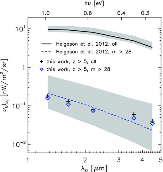
NIRB flux in the 1.25–4.5 μm wavelength range. The solid line is the flux from all galaxies from the ‘default’ model in Helgason et al. (2012), while the dashed line is the remaining flux after removal of all sources brighter than mlim = 28. The grey regions refer to the flux range between the ‘HFE’ and ‘LFE’ models in Helgason et al. (2012). As a comparison, we plot the flux from all galaxies with z > 5 in our work (crosses), and the flux after removal of sources down to mlim = 28 (diamonds). Before any galaxy removal, the flux from galaxies with z > 5 is only a few per cent of the overall flux in Helgason et al. (2012); that is, the low-redshift galaxies dominate. However, after removal of galaxies with mlim < 28, the flux from the remaining galaxies at all redshifts in Helgason et al. (2012) is comparable with that from the remaining galaxies with z > 5 in our work.
Before moving to fluctuations, we emphasize that the expected contribution of high-redshift galaxies (including Population III stars) to the NIRB flux is very small compared with the residual flux in the measurement of Matsumoto et al. (2005). These sources fall short of accounting for such a residual (∼60–6 nW m−2 sr−1 in the wavelength range 1.4–4 μm). It should be recalled that the flux measured by Matsumoto et al. is likely to be still dominated by incomplete zodiacal light subtraction, as discussed by Thompson et al. (2007a), who concluded that no residual flux is present. Considering the difficulties in modelling the zodiacal light accurately, the residual flux measurements are currently not very useful for constraining models. Therefore, we will base all the conclusions in the present paper on the analysis of fluctuations only (see below).
The fluctuations of the NIRB after subtracting galaxies down to the detection limits of observations, |$\sqrt{l(l+1)C_l/(2\pi )}$|, at λ0 = 1.6, 2.4, 3.6 and 4.5 μm are shown by the thick solid line in each panel of Fig. 5. The contribution from z > 5 faint galaxies, which is studied in this work, and the contribution from z < 5 galaxies, which is calculated by following the reconstruction of Helgason et al. (2012), are shown by the dashed line and the dash–dotted line respectively. Unless the limiting magnitude is very faint so that the relative fraction of the contribution of high-redshift galaxies is larger as in the upper left panel, the contribution of z > 5 galaxies is negligible compared with the z < 5 galaxies; that is, the total amplitude (solid line) coincides with that of z < 5 galaxies (dash–dotted line). To account for the uncertainties of the faint-end of LFs, Helgason et al. (2012) considered two models of the faint-end of LFs (adopted for low-redshift faint galaxies here), which are likely to bracket the real case. Considering this, we show the range of the total power spectrum by the shaded regions. We also plot observations at the corresponding wavelength in each panel, as filled circles with error bars, which are from Thompson et al. (2007a) (1.6 μm), Matsumoto et al. (2011) (2.4 μm) and Cooray et al. (2012b) (3.6 and 4.5 μm). The measurements of Cooray et al. (2012b) agree well with the observations of Kashlinsky et al. (2012) at the same wavelength, but extend to larger angular scales. In the theoretical predictions, we remove the bright sources by selecting a limiting magnitude at each wavelength to obtain the shot-noise level of the remaining fainter galaxies (including both low-redshift and high-redshift ones, but the latter is almost negligible) that matches each measurement, namely mlim = 26.7, 23.2, 23.9 and 23.8 respectively. The first two values are the same as in Helgason et al. (2012).
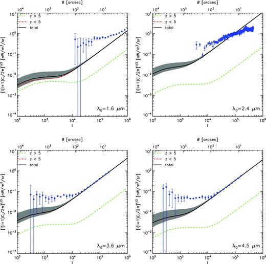
Angular power spectrum of NIRB fluctuations at various (observer-frame) wavelengths, as labelled in each panel; both the galaxy clustering and the shot noise are included. The dashed lines represent the contribution from the high-redshift galaxies studied in this work, while the dash–dotted lines represent the contribution from the low-redshift galaxies reconstructed by Helgason et al. (2012) (their ‘default’ model). The solid lines are the sum of these. Note that in all panels except the upper left one, where the limiting magnitude is very faint, the dash–dotted line and the solid line are almost identical. The shaded regions are the ranges of the total power spectrum when considering various faint-ends of the LFs, which are likely to bracket the real case (the ‘HFE’ and ‘LFE’ models in Helgason et al. 2012). We also plot the observations at wavelengths 1.6 (Thompson et al. 2007a), 2.4 (Matsumoto et al. 2011), 3.6 and 4.5 μm (Cooray et al. 2012b, which agree well with other recent measurements, i.e. Kashlinsky et al. 2012, but extend to larger angular scales) by filled circles with error bars. In all our theoretical predictions, we have removed the bright sources to reach the shot-noise level that matches each measurement – see text.
At small scales where the shot noise dominates, the model predictions should match the observations, as shown in the 3.6- and 4.5-μm panels. In the 2.4-μm panel, there is some discrepancy at small scales; this is because the suppression of the power by beam effects is not corrected in the observational data. Regarding the 1.6-μm case, a footnote in Helgason et al. (2012) notes that images at other wavelength are used to subtract bright sources, so there is spread on the limiting magnitudes.
From the figure, we also see that the contributions of the z > 5 galaxies (dashed lines) exceed the shot-noise level at large angular scales (l < 104). This means that the NIRB fluctuations do have the potential to provide information on the nature of the undetected reionization sources. However, the predicted amplitudes are only ∼(2–4) × 10−3 nW m−2 sr−1, which is even much smaller than the contribution from low-redshift faint galaxies, and both the high-redshift and low-redshift contributions are much smaller than the observed values, which are at the ∼0.1 nW m−2 sr−1 level. Even considering the uncertainties about the faint-end of LFs, the difference is still significant, again indicating the existence of one or more unknown component(s) that we are missing. Somewhat surprisingly but interestingly, the missing component has a clustering signal very similar to that of the high-redshift galaxies, and extends to degree angular scales. Obviously, this component/foreground must be identified before we can make further progress and use the NIRB to study reionization sources.
Next, we define the fluctuation amplitude |$\delta F = \sqrt{l(l+1)C_l/(2\pi )}$|, and plot its ratio to |$F = \nu _0I_{\nu _0}$| in Fig. 6. Such relative fluctuation is almost independent of λ0 (see also Fernandez et al. 2010). δF/F ∼ 4 per cent at l = 2000, with only a slight deviation of the 1.6-μm band, for which it is somewhat lower than in redder bands, as a consequence of a deeper (mlim ∼ 27) galaxy removal. Nicely, the relative fluctuation agrees with that found by Fernandez et al. (2010) and Cooray et al. (2012a). In addition, δF/F increases with zmin; that is, high-redshift sources have higher relative fluctuations. For example, δF/F = 7 per cent for zmin = 8.0, while it reaches 12 per cent if zmin = 12.0 is adopted. It reflects the more biased spatial distributions of higher-redshift sources. The relative fluctuation δF/F is only weakly dependent on the intrinsic properties of galaxies (Fernandez et al. 2010), but more so on the spatial clustering features. Thus, δF/F is a key indicator for identifying NIRB sources. In practice, however, it is hard to obtain an accurate absolute flux.
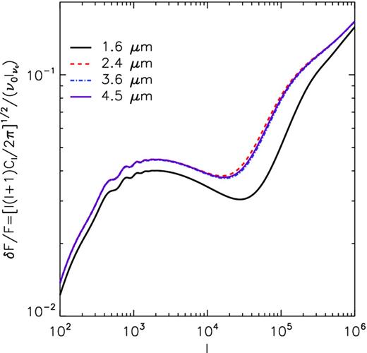
Ratio of δF/F as a function of l for four wavelengths.
The spectrum of the fluctuations, δF(λ0) from all galaxies with z > 5 at l = 2000, shown in Fig. 7, has a slope λp0, with p = −1.4 above 1 μm. Such a slope is essentially the same as that of the flux, reflecting the above-mentioned wavelength independence of δF/F.
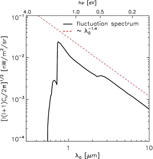
Spectrum of the NIRB (contributed by all z > 5 galaxies) fluctuations (solid line) at l = 2000; the dashed line shows a λ− 1.40 law.
CONCLUSIONS
By combining high-resolution cosmological N-body/ hydrodynamical simulations and an analytical model, we have predicted the contributions to the absolute flux and fluctuations of the NIRB by high-redshift (z > 5) galaxies, some of which harbour Population III stars. This is the most robust and detailed theoretical calculation undertaken so far, as we simultaneously match the LFs and reionization constraints. The simulations include the relevant physics of galaxy formation and a novel treatment of chemical feedback, by following the metallicity evolution and implementing the physics of the Population III/Population II transition based on a critical metallicity criterion. They reproduce the observed UV LFs over the redshift range 5 < z < 10, and extend the LFs to faint magnitudes far below the detection limit of current observations.
We directly calculate the stellar emissivity from the simulations. We use Starburst99 to generate metallicity- and age-dependent SED templates, and then calculate the luminosity for each galaxy according to its current star formation rate, stellar age and metallicity, instead of using a constant-metallicity and average main sequence spectrum template. Except for the mass range of the IMF, which is fixed in the simulation, there are no other free parameters in the calculation of the emissivity.
By comparing the number of ionizing photons produced per baryon in collapsed objects, f⋆Nγ, in the simulation and the ionizing photon rate, Nion ≈ fescf⋆Nγ, deduced from observationally constrained reionization models, we obtained the evolution history of the escape fraction of ionizing photons, fesc(z). We find fesc ∼ 1 at z > 11, decreasing to ∼0.05 at z = 5. This escape fraction is used to renormalize the nebular emission of Population III and Population II stars in the emissivity.
Population III stars are unlikely to be responsible for the observed NIRB residual, and their contribution is very small, making up <1 per cent of the total absolute flux in our calculation. This is the natural result of the much lower star formation rate of Population III stars compared with Population II stars in the simulation, as metals from even a single Population III star could enrich a large amount of the surrounding gas above the critical metallicity (Tornatore et al. 2007b). The formation of Population III stars is regulated by such a chemical feedback mechanism, which limits their contribution to the NIRB. However, a rapid Population III–Population II transition brings also a little advantage in terms of integrated emissivity, owing to the longer lifetime of Population II stars (Cooray et al. 2012a).
We predict that in the wavelength range 1.0–4.5 μm, the NIRB flux from z > 5 galaxies (and their Population III stars) is ∼0.2–0.04 nW m−2 sr−1, while the fluctuation strength is about δF = 0.01–0.002 nW m−2 sr−1 at l = 2000. If we remove galaxies down to mlim = 28, the above flux level is only slightly reduced; however, from comparison with Helgason et al. (2012), we find that the flux from z < 5 galaxies dramatically decreases and the remaining becomes comparable to the predicted signal of z > 5 galaxies. This implies that in principle it is possible to obtain the signal from reionization sources by subtracting galaxies down to a certain magnitude.
The relative fluctuation amplitude, δF/F, at l = 2000 is ∼4 per cent, almost independent of the wavelength. This ratio may be helpful in investigating the clustering features of the sources that contribute to the NIRB, as the intrinsic properties of galaxies almost cancel out. Despite the difficulties in measuring the absolute flux accurately, it could be treated as a quality indicator in the data reduction process: if a much higher/lower ratio is obtained from the data, this might suggest that a more careful analysis is required to extract the genuine contribution from reionization sources.
In spite of our model being consistent with the observed LFs and reionization data, thus offering a robust prediction of the NIRB contribution from high-redshift galaxies that probably reionized the Universe, a puzzling issue remains: the predicted fluctuations are considerably lower than the observed values, indicating that in addition to the contribution from the expected high-redshift galaxy population (and Population III stars), we should invoke some other – as yet unknown – missing component(s) or foreground(s) that dominates the currently observed source-subtracted NIRB. Moreover, the angular clustering of this missing component must be very similar to that of the high-redshift galaxies and extend to degree scales. Obviously, this component/foreground must be identified and removed before we are ready to exploit the NIRB to study reionization sources. On the other hand, sources located at 5 < z < 8 provide about 90 per cent of the flux from all sources with z > 5 in our simulation; most of them are faint galaxies currently undetected by deep surveys. Thus, if the above-mentioned additional spurious sources/foregrounds can be removed reliably, the NIRB will become the primary tool for investigating the properties of reionizing sources.
It is a pleasure to acknowledge intense discussions and data exchange with A. Cooray, K. Helgason, E. Komatsu, T. Matsumoto, R. Thompson, S. Kashlinsky, S. Mitra and T. Choudhury. AF thanks UT Austin for support and hospitality as a Centennial B. Tinsley Professor and for the stimulating atmosphere of the NIRB Workshop organized by the Texas Cosmology Center. BY and XC also acknowledge support from NSFC grant 11073024, MoST Project 863 grant 2012AA121701, and the Chinese Academy of Science Knowledge Innovation grant KJCX2-EW-W01.
A significant contribution from high-redshift mini-quasars powered by accretion onto intermediate-mass black holes with spectra similar to local ultra-luminous X-ray sources is disfavoured on the basis of the unresolved X-ray background intensity constraints (Salvaterra, Haardt & Ferrara 2005), unless these objects are highly absorbed by the surrounding gas.
The dust absorption in the host galaxy may lower its luminosity in the rest-frame UV band, and therefore reduce the contribution to the NIRB. However, as shown by Salvaterra et al. (2011), for the high-redshift dwarf galaxies considered by us here, this effect is negligible. The absorption is possibly important for very massive objects at the bright end of LFs, but their contribution to the emissivity is very small. The lack of significant dust absorption is further supported by the observed very blue UV-continuum slopes of high-redshift galaxies reported in Bouwens et al. (2009). Therefore, we ignore the effect of dust in the current calculations. Furthermore, we will show later that the high-redshift galaxies are inadequate for explaining the amplitude of the observed fluctuations; consideration of the dust absorption would only strengthen this point.
Note the different dimensions of qIIH and qIIIH: the former corresponds to per unit star formation rate, while the latter corresponds to per unit stellar mass.
REFERENCES
APPENDIX A: AN ANALYTICAL DERIVATION OF THE EMISSIVITY
In our work, the mass range of Population II stars is 0.1–100 M⊙, while the fitted formula of the main sequence age used in Fernandez & Komatsu (2006), Fernandez et al. (2010) and Cooray et al. (2012a) (taken from Schaerer 2002) is based on data of massive stars. To avoid introducing more uncertainties, in this comparison we adopt a mass range 1–100 M⊙ for Population II stars. We checked that for Population II stars with mass 1 M⊙, the fitted main sequence age still agrees with Girardi et al. (2000).
Because Population II stars are found to contribute much more than Population III stars to the NIRB (see Fig. 3), and stellar emission is the dominant component, we neglect here the nebular emission. Lν can then be represented by a blackbody spectrum, and we truncate it at hν = 13.6 eV (Fernandez & Komatsu 2006; Fernandez et al. 2010; Cooray et al. 2012a).
We plot the emissivity at z = 10 calculated by different methods in Fig. A1 for a star formation efficiency f⋆ = 0.01 and a minimum mass Mmin = 106 M⊙. It is not surprising that ‘Approximation 2’ overestimates the emissivity, as it assumes that none of the stars die. However, we find that for the stellar mass range 1–100 M⊙, ‘Approximation 1’ also overestimates the emissivity when hν < 8 eV, because of the contribution of low-mass stars whose lifetime is even longer than the age of the Universe at that redshift, so that τ(m) < tSF is not fulfilled. However, high-energy photons come mainly from massive stars, which satisfy τ(m) < tSF. So at high energies, ‘Approximation 1’ results agree well with the full analytical solution. The ‘Hybrid’ approximation is more accurate through the whole range of energy shown in Fig. A1, although the results still deviate from the full analytical solution.
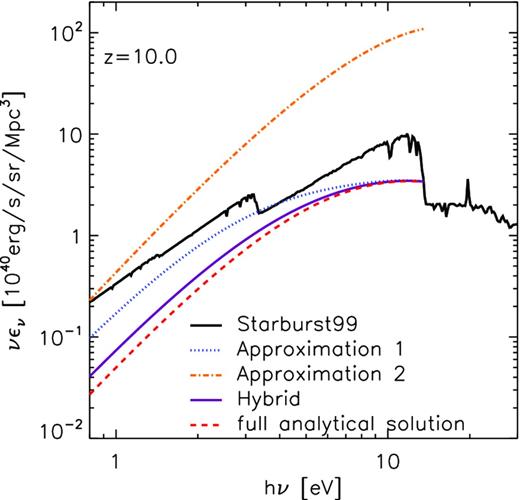
Emissivity of Population II stars at redshift 10.0. The solid line is the result obtained using the spectrum template from Starburst99 used here; the dotted line is for ‘Approximation 1’; the dash–dotted line refers to ‘Approximation 2’. The dash–dotted–dotted–dotted line corresponds to the ‘Hybrid’ approximation; finally the dashed line refers to the full analytical solution of equations (A1)–(A4) using fitting formulae (see text).
However, the emissivity calculated from the template of Starburst99 is still higher than the results obtained from the full analytical solution of equations (A1)–(A4) with fitting formulae. This is mainly due to the full stellar evolutionary tracks used by Starburst99, which extend beyond the zero-age main sequence (ZAMS) stage. For example, the luminosity of a 7 M⊙ star with metallicity 1/50 Z⊙ at the end of the main sequence is three times as large as the ZAMS luminosity; at the end of its evolution, the luminosity is ∼10 times higher than the ZAMS luminosity. The analogous value for a 100 M⊙ star of the same metallicity is about 2 times the ZAMS luminosity.
