


Abstract
Understanding the processes that can destroy H2 and H− species is quintessential in governing the formation of the first stars, black holes and galaxies. In this study, we compute the reaction rate coefficients for H2 photodissociation by Lyman–Werner photons (11.2–13.6 eV) and H− photodetachment by 0.76 eV photons emanating from self-consistent stellar populations that we model using publicly available stellar synthesis codes. So far, studies that include chemical networks for the formation of molecular hydrogen take these processes into account by assuming that the source spectra can be approximated by a power-law dependence or a blackbody spectrum at 104 or 105 K. We show that using spectra generated from realistic stellar population models can alter the reaction rates for photodissociation, kdi, and photodetachment, kde, significantly. In particular, kde can be up to ∼2–4 orders of magnitude lower in the case of realistic stellar spectra suggesting that previous calculations have overestimated the impact that radiation has on lowering H2 abundances. In contrast to burst modes of star formation, we find that models with continuous star formation predict increasing kde and kdi, which makes it necessary to include the star formation history of sources to derive self-consistent reaction rates, and that it is not enough to just calculate J21 for the background. For models with constant star formation rate, the change in shape of the spectral energy distribution leads to a non-negligible late-time contribution to kde and kdi, and we present self-consistently derived cosmological reaction rates based on star formation rates consistent with observations of the high-redshift Universe.
1 INTRODUCTION
The first generation of stars (Population III or Pop III) in the early universe are believed to form from cooling and subsequent collapse of primordial unenriched gas (e.g. Tegmark et al. 1997; Bromm, Coppi & Larson 1999). At temperature below ∼8000 K, primordial gas in the early Universe cools most efficiently via molecular hydrogen to temperatures of ≈ few 100 K at which point the Jeans mass can be exceeded and gravitational runaway collapse of gas can proceed (e.g. Omukai & Nishi 1998; Abel, Bryan & Norman 2002; Yoshida et al. 2003). This channel of cooling is of importance for the formation of the Pop III stars in mini-haloes at z ≥ 10, which kick-start the metal enrichment of the intergalactic medium and interstellar medium (e.g. Maio et al. 2011; Muratov et al. 2013), and subsequently lead to Population II (Pop II) star formation (SF). The complete suppression of H2 cooling has been argued to lead to the formation of black holes via the direct collapse of Jeans-unstable gas clouds of ∼105–6 M⊙ in atomic cooling haloes (e.g. Rees 1978; Omukai 2001; Begelman, Volonteri & Rees 2006; Spaans & Silk 2006; Shang, Bryan & Haiman 2010).
It is clear from above that the abundance of H2 molecules will significantly influence structure formation in the early Universe, and that accurate modelling of its formation and destruction is essential for theoretical studies that explore the same and significant work as has been done in modelling the formation of H2 molecules in a cosmological context (e.g. Stecher & Williams 1967; Allison & Dalgarno 1970; Dalgarno & Stephens 1970; de Jong 1972).
The reaction rate coefficients for the destruction of these two species have been derived in the literature by assuming that sources have spectra that can be approximated as power law or a blackbody type (e.g. Draine & Bertoldi 1996; Abel et al. 1997; Galli & Palla 1998a, 1998b; Omukai 2001). However, the spectral energy distribution (SED) of stars shows a strong time dependence in its normalization and shape at the relevant energies (e.g. Leitherer et al. 1999; Schaerer 2002). While the former is generally accounted for (e.g. Dijkstra et al. 2008; Agarwal et al. 2012; Latif et al. 2014; Visbal et al. 2014), the latter has been completely neglected so far. Previous estimates have been based on thermal spectra, mostly at a temperature of 104 K (T4) that is argued to mimic a Pop II-type stellar population, and at 105 K (T5) that mimics a Pop III-type population (Omukai 2001; Shang, Bryan & Haiman 2010; Wolcott-Green, Haiman & Bryan 2011). The aim of this paper is to derive reaction rate coefficients for the destruction of H2 and H−, based on stellar synthesis models representative of stellar populations in galaxies, and to investigate their impact on the formation and destruction of H2 molecules.
The paper is organized as follows. We will outline the methodology in Section 2, followed by the results that are presented in Section 3. Finally, the conclusions and a critical discussion of the implication of the work presented in this study are given in Section 4.
2 METHODOLOGY
The spectral parameter, β (α), introduces the sensitivity of the reaction rate on the SED of the source with respect to a source with a flat spectrum.
With above definitions, the time dependence of the reaction rates on the SED is split up into two components: one that is equal for both (J21) and just reflects the amount of UV photons depending on the age of the stellar population, and the other (α and β, respectively) that is sensitive to the change in the shape of the SED. The constants κde and κdi carry the units of s−1, and reflect the efficiency of the reactions.
2.1 H2
2.2 H−
Defining κde as the value of kde at J21 = 1, i.e. Ln = 1 × 10⁻²¹ erg s−1 cm−2 sr−1, constant for all frequencies and in time (Omukai 2001, appendix A), the integral in equation (13) can be solved to give κde = 1.1 × 10⁻¹⁰ s−1.
Using the above formulation, one obtains α ≈ 8 (2000) for a power-law-type (T4) spectrum, as shown by Omukai (2001).
Properties of the stellar populations analysed in this work and their corresponding references. The IMF slope is of the form ξ ∝ m−α, and the mass interval is listed in the form [Mmin, Mmax]. The total stellar mass is proportional to the stellar age in the case of a continuous SFR mode, and for the burst modes, the SFR is assumed to occur in bursts at each time interval.
| Reference | IMF | Slope | Mass interval | Mtot | SFR | Name | |
|---|---|---|---|---|---|---|---|
| (M⊙) | (M⊙) | (M⊙ yr−1) | |||||
| Pop III | ST99a | Salpeter | 2.35 | 50, 500 | 106 | Burst | ST99_III |
| Pop II | ST99b | Chabrier | 2.3,2.3 | [0.1, 1],[1, 100] | 106 | Burst | ST99_Cb |
| Pop II | ST99 | Salpeter | 2.35 | 1, 100 | ∝t | 1 | ST99_Sc |
| Pop II | ST99 | Salpeter | 2.35 | 1, 100 | 106 | Burst | ST99_Sb |
Note:aCode was modified to include the modified IMF (personal communication with Daniel Schaerer). bCode was modified to include the IMF and a lower metallicity limit.
Sample data table: |$\rm \rm log_{10}(\beta )$| for different Pop II-type models analysed in this work. Complete data table can be downloaded from the source.
| ST99_Cb | ST99_Sb | ST99_Sc | |||||||
|---|---|---|---|---|---|---|---|---|---|
| Age | Z = 0.0004 | 0.005 | 0.05 | Z = 0.001 | 0.008 | 0.04 | Z = 0.001 | 0.008 | 0.04 |
| (Myr) | β | β | β | β | β | β | β | β | β |
| 1.00 | 0.07 | 0.08 | 0.06 | 0.34 | 0.34 | 0.36 | 0.34 | 0.34 | 0.34 |
| 2.00 | 0.06 | 0.07 | 0.06 | 0.34 | 0.38 | 0.41 | 0.34 | 0.35 | 0.36 |
| … | |||||||||
| 800.00 | 4.01 | 2.66 | 2.07 | 3.90 | 1.85 | 1.95 | 0.65 | 0.61 | 0.56 |
| 900.00 | 4.04 | 2.40 | 2.18 | 3.90 | 1.80 | 2.77 | 0.65 | 0.61 | 0.56 |
Sample data table: |$\rm \rm log_{10}(\alpha )$| for different Pop II-type models analysed in this work. Complete data table can be downloaded from the source.
| ST99_Cb | ST99_Sb | ST99_Sc | |||||||
|---|---|---|---|---|---|---|---|---|---|
| Age | Z = 0.0004 | 0.005 | 0.05 | Z = 0.001 | 0.008 | 0.04 | Z = 0.001 | 0.008 | 0.04 |
| (Myr) | α | α | α | α | α | α | α | α | α |
| 1.00 | −0.19 | −0.23 | −0.31 | −0.12 | −0.13 | −0.10 | −0.11 | −0.13 | −0.12 |
| 2.00 | −0.20 | −0.26 | −0.26 | −0.13 | −0.12 | −0.03 | −0.12 | −0.13 | −0.10 |
| … | |||||||||
| 800.00 | 6.33 | 8.36 | 11.65 | 6.04 | 8.63 | 11.72 | 0.88 | 0.96 | 0.99 |
| 900.00 | 6.55 | 8.68 | 12.01 | 6.37 | 9.00 | 12.79 | 0.89 | 0.97 | 1.01 |
2.3 Stellar populations
We use the publicly available stellar synthesis code starburst99 (Leitherer et al. 1999), and Schaerer (2002) to model Pop II- and Pop III-type stellar populations with different star formation histories (SFHs). The properties of each of the models analysed in this study are listed in Table 1. In brief, we generate Pop II SEDs for either Salpeter or Chabrier initial mass functions (IMFs) using single-burst models that form 106 M⊙ instantaneously, or continuous SF models with 1 M⊙ yr−1. In addition, we model Pop III SEDs using a Salpeter IMF with a high-mass end of 500 M⊙.3
Sample data table: α and β for the Pop III-type model (ST99_III) analysed in this work. Complete data table can be downloaded from the source.
| Age | ||
|---|---|---|
| (Myr) | α | β |
| 1.00 | 1.71 | 0.97 |
| 1.05 | 1.68 | 0.97 |
| … | ||
| 3.50 | 0.91 | 1.07 |
| 3.55 | 0.93 | 1.16 |
| Age | ||
|---|---|---|
| (Myr) | α | β |
| 1.00 | 1.71 | 0.97 |
| 1.05 | 1.68 | 0.97 |
| … | ||
| 3.50 | 0.91 | 1.07 |
| 3.55 | 0.93 | 1.16 |
3 RESULTS
Here we present the results of our implementation. We find that the spectral parameters are extremely sensitive to the age of the stellar population that is producing the photons.4 We will also discuss in detail the impact that these spectral parameters have on the final reaction rates, and the interplay with J21.
3.1 Pop III
For our case with the Pop III-type population (ST99_III) where a single burst of star formation rate (SFR) is used, we find little variation in the value of the spectral parameters over the age of the stellar population considered, as seen in Figs 1 and 2. For our mass range of Pop III stars considered, 50–500 M⊙, the age of the population extends over ≈1–3.6 Myr only. Although the spectral parameters do not vary as dramatically as in the Pop II-type cases (see Figs 1 and 2), in the first 106 yr ST99_III produces higher values for kdi and kde than a comparable burst for Pop II stars as shown in Figs 3 and 4. This does not come as a surprise given that the number of massive stars is larger for our choice of Pop III IMF.
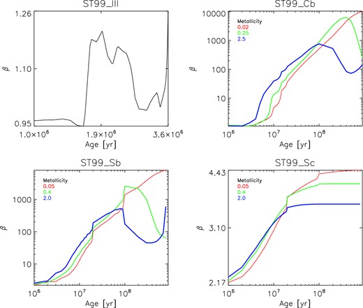
The β parameter for H2 dissociation from the different stellar populations analysed in this study. Note that the metallicities are quoted in solar units with Z⊙ = 0.02. In the bottom-right panel, a continuous SFR of 1 M⊙ yr−1 is employed, whereas in the rest of the panels a single burst of 106 M⊙ is used to model the SFR (see Table 1).
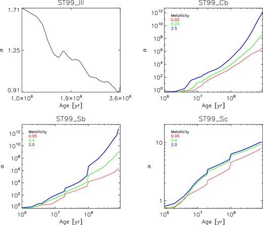
The α parameter for H− photodetachment from different stellar populations analysed in this study (see the caption for Fig. 1 for more details).
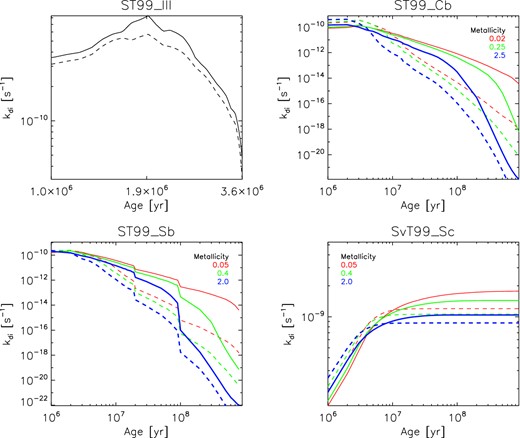
The reaction rate coefficient kdi for H2 photodissociation computed at a distance of 5 kpc (physical) from a given stellar population (see the caption for Fig. 1 for more details). The dashed lines are computed for β = 0.1 (top-left panel) and β = 3 (rest) corresponding to a T5 and T4 spectrum, respectively, with the same J21 for the stellar populations.
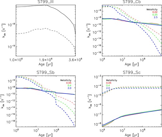
The reaction rate coefficient kde for H− photodetachment computed at a distance of 5 kpc (physical) from a given stellar population (see the caption for Fig. 1 for more details). The dashed lines are computed for α = 8 (top-left panel) and α = 2000 (rest) corresponding to a T5 and T4 spectrum, respectively, with the same J21 derived from the stellar populations.
3.2 Pop II
Models with bursts show a stronger dependence of the spectral parameters on the age of the population beyond a few Myr (see ST99_Cb and ST99_Sb in Fig. 1) than the ones with a continuous mode of SF. Initially, the corresponding bands evolve similar to the band at 13.6 eV. However, after a few million years the output at this wavelength drops more severely and we find a several-orders-of-magnitude increase in β and α. The time dependence of α is stronger than that of β because the change in the shape of the SED with respect to 13.6 eV is stronger at 0.76 eV than in the LW bands. While these changes are significant, one needs to calculate kde and kdi to gauge the impact on the reaction rates, as J21 is an equally strong function of time in the opposite direction to α and β, and could potentially compensate for any time evolution. In Figs 3 and 4, we show kde and kdi as a function of time for a source located 5 kpc (physical) away for different metallicities. This involves computing J21 for a given age and metallicity for the underlying stellar population, normalized to either 106 M⊙ or an SFR of |$1 \, \mathrm{M}_{{\odot }}\ \rm yr^{-1}$|. Dashed lines are for reaction rates computed using the spectral parameters for a T5 spectrum for the top-left panel, meant to mimic a Pop III-type population, and T4 for the rest of the panels, meant to represent Pop II stars, with the same J21 derived for the corresponding stellar models.
As expected, the impact of using SEDs from stellar population models is much stronger for the photodetachment than for photodissociation. This is because the temporal evolution of the SED is generally normalized to 13.6 eV which is in the LW band, thus making the effect less pronounced for kdi. For both the burst and continuous modes, within the first ∼ 10 Myr, kdi is only a factor of few higher in the T4 case, after which it falls ∼1–2 orders of magnitude below the realistic spectra. However, by that time the UV output in terms of J21 has dropped off significantly for the bursty models, suggesting that H2 photodissociation will be mostly affected in this case within the first 10 Myr. However, for continuously star-forming galaxies the maximal destruction of H2 occurs after ∼10 Myr, and the blackbody predictions are similar to that of the stellar SEDs. Galaxies with constant or even increasing SFHs as predicted by galaxy formation models (e.g. Finlator, Oppenheimer & Davé 2011; Khochfar & Silk 2011) will thus have H2 photodissociation occurring more efficiently as predicted by simple blackbody spectra.
The T5 spectrum is over an order of magnitude efficient in photodetaching H− as compared to the Pop III-type model analysed in this study. The T4 spectra, however, produce a kde that is more than three orders of magnitude higher than the burst modes, but only at stellar ages of <50 Myr, after which the T5 spectrum drops off steeply. This accentuates the role of older stellar populations if one considers bursty SF modes, as the drop in kde between 1 Myr and 1 Gyr for the burst modes analysed here is only about two orders of magnitude, but is over 13 orders of magnitude for the T4 spectrum. However, as compared to the case with a cosmic star formation rate (CSFR), the T4 spectrum results in a detachment rate that is ∼2–3 orders of magnitude higher for the entire age of the stellar population. The implications of this deviation of the detachment rates can be severe for processes like direct-collapse black hole (DCBH) formation, where kde plays a pivotal role in determining the critical level of LW specific intensity needed from Pop II stars to fully suppress H2 cooling.
3.3 Inexistence of a universal Jcrit
The collapse and thermodynamic fate of pristine gas are governed by the reactions discussed in this study [equations (11) and (15)], which are extremely sensitive to the age and SFH of the stellar population in galaxies producing the photons and the level of J21 as shown above. Thus, merely knowing the value of J21, which is calculated at 13.6 eV only, is not sufficient to predict if the gas is free of molecular hydrogen. Even for the case of suppression of Pop III SF by a global LW background (e.g. Glover & Brand 2001; Machacek, Bryan & Abel 2001; O'Shea & Norman 2008), the time dependence on the spectral parameters α and β must be accounted for.
We argue that the most drastic outcome of our work is the possibility of the absence of a universal Jcrit required for direct collapse. Previous studies have shown that the value of Jcrit is extremely sensitive to the rate of reactions (3) and (4) at number densities of <104 cm−3 (Omukai 2001; Shang et al. 2010; Wolcott-Green et al. 2011), where a T4- or T5-type irradiating source was assumed. However, a given value of J21 could be produced by stellar populations with various combinations of their properties such as age, metallicity, stellar mass and SFR. Depending on the combination of these variables, one could obtain a large range for the value of the spectral parameters (see Figs 1 and 2) and the corresponding value for the reaction rates for a fixedJ21. Based on this, we argue that the net formation rate of H2, kform (see equation 5), is a function of the stellar age, metallicity and SF mode. Thus, for a given value of kform (or kde and kdi), there is a degeneracy in the parameter space |$[(M_*, \dot{M_*}),\ \mathrm{Z}_{\odot },\ t]$| that determines the value of the reaction rates.
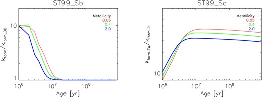
Ratio of kform derived in our work to that in the literature for a T4 spectrum, assuming that nH = 103 cm−3, and for the same value of J21 used in Figs 3 and 4. The ratio being larger than unity demonstrates that the spectra analysed in this work are less efficient in suppressing H2 formation, especially at low densities via the H− channel.
The deviation of the ratio from unity arises due to the dependence of kde on stellar age that we have demonstrated in this study, a variation that has been previously overlooked by assuming a constant value of the photodetachment rate (kde,BBT4) for T4-type spectra. We find that for a given value of J21, H2 forms more efficiently in the case of the spectra considered in this study, hinting at the need for a higher Jcrit.
3.4 Implementation
In the derivation of the spectral parameters and reaction rates, the definition of Ln and J21 must be consistent with each other in order to avoid spurious results, i.e. difference of over five orders of magnitude in the reaction rates. The difference can be attributed to the fact that Lν is not flat in the LW range for realistic spectra, such as the ones considered in this study. For instance, in our calculations, Ln is the spectrum normalized to its own value at 13.6 eV; thus, J21 is defined at 13.6 eV as well, and any other definition of J21 would lead to inconsistencies. Also, while using equations (11) and (15), the reader must renormalize J21 by a factor of |$\psi =\frac{M_*}{10^6\, \mathrm{M}_{{\odot }}}$| or |$\frac{\dot{M}_*}{1\, \mathrm{M}_{{\odot }}\,{\rm yr}^{-1}}$|, where M★ and |$\dot{M}_*$| denote the user-specified stellar mass and SFR for the underlying stellar population.
3.5 Cosmic values for kdi and kde
We compute the redshift evolution of the reaction rates, kde and kdi, using the approach outlined in this work (i.e. dependence on metallicity, stellar age, SF mode), and on the basis of the fiducial model of Agarwal et al. (2012), which reproduces the observed cosmic SFR in the high-redshift Universe. For their fiducial case and assuming that the Pop II stars in their work have Z = 0.05 Z⊙, we use their modelled SFHs of individual galaxies and the ST99_Sb case to compute the reaction rates.
The result of our computation for the global evolution of the reaction rates is plotted in Fig. 7. The reaction rates are highest at later times, due to the role that older stellar populations play in photodetachment and photodissociation. Given that the semi-analytical model of Agarwal et al. (2012) matches the observational constraints on the CSFR and stellar mass functions, the reaction rate curves represent the average cosmic value of the H− and H2 destruction in the presence of an LW background emanating from Pop II stars.
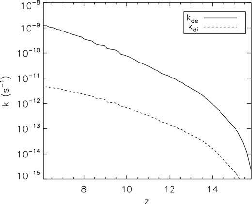
Cosmic averaged photodissociation and photodetachment rates computed as a function of redshift using the spectral parameters derived in this study, and Jbg,II derived on the basis of Agarwal et al. (2012).
4 CONCLUSION AND DISCUSSION
In this study, we have demonstrated that using stellar synthesis codes instead of the commonly assumed T5 or T4 thermal blackbody spectra to model the SEDs of Pop III and Pop II stellar populations can have a significant impact on the destruction of H2 and H−. We find that the spectral parameters β (α) can vary over 5 (12) orders of magnitude depending on the age of the stellar population. The reaction rates themselves however vary only over few orders of magnitude due to the interplay of the spectral parameters with J21 that goes into computing the rates.
It is clear that assuming that LW photons are being produced by only young stellar populations with ages 1–10 Myr can lead to an underestimation in the value of the reaction rates. For a given stellar mass, older stellar populations in a continuously star-forming galaxy are more efficient in both photodissociating H2 and photodetaching H− than stars that are assumed to be produced in instantaneous bursts. In the case of photodetachment of H−, the reaction rate increases with stellar age for the continuous mode, as compared to the bursty mode where it falls off steeply after 10 Myr. For photodetachment of H2 however, the reaction rate plateaus after 10 Myr for the continuous mode and, again, falls off steeply (more than 10 orders of magnitude) for the bursty mode. Thus, it becomes imperative to know the age, SFH and metallicity of the stellar population that is assumed to be the irradiating source, and knowing the value of J21 by itself is not enough.
Comparing the burst-mode models analysed here to blackbody curves, we find that photodissociation rate of H2, i.e. kdi, shows little difference at <10 Myr for Pop II stars. After 10 Myr however, the T4 photodissociation rate drops off rapidly and can be up to four to five orders of magnitude lower than the rate derived from stellar synthesis codes. However, the difference is minimal for the case with a continuous SF mode. For the photodetachment of H−, i.e. kde, the difference is quite large and pronounced. At <50 Myr, the photodetachment rates from the T4 spectra are three to four orders of magnitude higher than in the cases with a burst mode of SF, after which the trend reverses and they drop off steeply with respect to the stellar models. For the continuous mode of SF, the T4 photodetachment rate is three to four orders of magnitude higher than that derived from the stellar evolution model at any given age. This demonstrates that one must account for older stellar populations when studying processes that are affected by LW feedback. A recent study by Wolcott-Green & Haiman (2012) also suggests that smaller stars (few M⊙) tend to contribute significantly to H− photodetachment, and are thus critical to the LW feedback scenario governing Pop III SF in the early universe.
When studying the formation of the first stars and galaxies, where LW feedback is critical, reaction rates/rate coefficients derived here could serve as a more accurate prescription than what is available in the literature. We have derived cosmological average reaction rates, which can serve as self-consistent inputs in high-resolution zoom studies that do not follow the actual SFH in a large cosmological context.
The newly derived rate coefficients might alter the scenario of DCBH formation (e.g. Eisenstein & Loeb 1995; Oh & Haiman 2002; Bromm & Loeb 2003; Koushiappas, Bullock & Dekel 2004; Lodato & Natarajan 2006; Regan & Haehnelt 2009), where a critical level of LW specific intensity (Jcrit) is essential in suppressing H2 cooling. Previous studies have computed the critical level of LW intensity by assuming either a T4- or T5-type spectrum for the irradiating sources (Omukai 2001; Shang et al. 2010; Wolcott-Green et al. 2011); however, see also Latif et al. (2014) and Sugimura, Omukai & Inoue (2014) for more recent attempts. Repeating their analyses with the reaction rates presented in this study has the potential to significantly increase the value of Jcrit, thus presenting new challenges or avenues to the formation of quasars at z > 6.
BA would like to thank Kazu Omukai and Zoltan Haiman for discussions that sparked this project. The authors would like to thank Simon Glover and Andrew Davis for their inputs during the preparation of the manuscript. BA would also like to thank Jan-Pieter Paardekooper and Alessia Longobardi for useful discussions during the early stages of the manuscript. The authors also thank Jonathan Elliott and Laura Morselli for their comments on the draft.
Strictly speaking, LW radiation only corresponds to photons with energies between 11.2 and 13.6 eV. However, for the sake of convenience in the following, we will refer by LW radiation or radiation to photons responsible for photodetachment of H− as well.
The IMF of Pop III stars is heavily debated at this point going from flat to top-heavy (e.g. Hirano et al. 2014).
REFERENCES
SUPPORTING INFORMATION
Additional Supporting Information may be found in the online version of this article:
Table 2. Sample data table: |$\rm \rm log_{10}(\beta )$| for different Pop II-type models analysed in this work.
Table 3. Sample data table: |$\rm \rm log_{10}(\alpha )$| for different Pop II-type models analysed in this work.
Table 4. Sample data table: α and β for the Pop III-type model (ST99_III) analysed in this work.
Please note: Oxford University Press is not responsible for the content or functionality of any supporting materials supplied by the authors. Any queries (other than missing material) should be directed to the corresponding author for the paper.
