


Abstract
Cosmological shock waves play an important role in hierarchical structure formation by dissipating and thermalizing kinetic energy of gas flows, thereby heating the Universe. Furthermore, identifying shocks in hydrodynamical simulations and measuring their Mach number accurately are critical for calculating the production of non-thermal particle components through diffusive shock acceleration. However, shocks are often significantly broadened in numerical simulations, making it challenging to implement an accurate shock finder. We here introduce a refined methodology for detecting shocks in the moving-mesh code arepo, and show that results for shock statistics can be sensitive to implementation details. We put special emphasis on filtering against spurious shock detections due to tangential discontinuities and contacts. Both of them are omnipresent in cosmological simulations, for example in the form of shear-induced Kelvin–Helmholtz instabilities and cold fronts. As an initial application of our new implementation, we analyse shock statistics in non-radiative cosmological simulations of dark matter and baryons. We find that the bulk of energy dissipation at redshift zero occurs in shocks with Mach numbers around |$\mathcal {M}\approx 2.7$|. Furthermore, almost 40 per cent of the thermalization is contributed by shocks in the warm hot intergalactic medium, whereas ≈60 per cent occurs in clusters, groups, and smaller haloes. Compared to previous studies, these findings revise the characterization of the most important shocks towards higher Mach numbers and lower density structures. Our results also suggest that regions with densities above and below δb = 100 should be roughly equally important for the energetics of cosmic ray acceleration through large-scale structure shocks.
1 INTRODUCTION
The collapse of dark and baryonic matter during hierarchical large-scale structure formation releases gravitational energy and transforms it into kinetic energy. The bulk of the kinetic energy of the gas gets dissipated by cosmological shocks, heating the gas in virialized haloes (e.g. the intracluster medium, ICM) as well as in the warm-hot intergalactic medium (WHIM). Cosmological hydrodynamic shocks are collisionless; they are established due to plasma interactions by means of magnetic fields. They can themselves amplify magnetic fields and accelerate particles via diffusive shock acceleration (DSA; Axford, Leer & Skadron 1977; Krymskii 1977; Bell 1978a,b; Blandford & Ostriker 1978; Malkov & O'C Drury 2001) up to relativistic energies, producing cosmic rays.
Directly observing cosmological shocks is challenging, especially outside cluster cores where the X-ray emission is weak. An obvious approach is to look for jumps in the thermal gas quantities. In this way, and using exquisite X-ray data from the Chandra telescope, the first merger shocks have been confirmed in the bullet cluster (|$\mathcal {M}\approx 3$|; Markevitch et al. 2002; Markevitch 2006) and in the train-wreck cluster (|$\mathcal {M}\approx 2.1$|; Markevitch et al. 2005). Maps of the gas density and the temperature can be inferred from the luminosity and the spectrum of the X-ray radiation, respectively. Both are necessary in order to calculate a pressure map and confirm a shock. Furthermore, it is possible to directly measure a pressure jump by means of the thermal Sunyaev–Zel'dovich signal (Sunyaev & Zeldovich 1980). For example, steep pressure gradients have been detected inside R500 in the nearby Coma Cluster (Planck Collaboration X 2013). The location of the gradients coincides with temperature jumps, and two shocks with Mach numbers around |$\mathcal {M}\approx 2$| were reported in this way.
Shocks can also be observed indirectly at radio wavelengths. Diffusively shock-accelerated cosmic ray electrons in merger and accretion shocks produce synchrotron radiation, so-called radio gischt (Ensslin et al. 1998; Battaglia et al. 2009; Pinzke, Oh & Pfrommer 2013). This phenomenon has been observed in several clusters (see e.g. Clarke & Ensslin 2006; Bonafede et al. 2009; van Weeren et al. 2010; Brüggen et al. 2012, for a review of shocks in cluster outskirts and the associated features). Another radio source triggered by shocks is the radio phoenix (Enßlin & Gopal-Krishna 2001; Enßlin & Brüggen 2002). In this scenario, a shock overruns fossil radio plasma initially produced by an active galactic nucleus (AGN), compressing the plasma and reviving its radio emission. A radio phoenix can reveal large-scale accretion shocks and has been reported for the Perseus Cluster (Pfrommer & Jones 2011).
The motivation for observing shocks is manifold. First of all, supersonic flows and their associated shocks allow the study of thermalization patterns and energetics of phenomena at a broad range of spatial scales. This includes accretion shocks onto clusters, mergers of galaxies and galaxy clusters, winds and jets of AGN, as well as stellar winds and supernovae. Secondly, observations of supernova remnants provide evidence for the creation of non-thermal cosmic ray particles at these locations. Cosmic ray protons can collide with thermal protons of the interstellar medium producing pions, which subsequently decay and release γ-radiation. The pion decay and hence the acceleration of cosmic ray protons has been confirmed for several supernova remnants (e.g. Giuliani et al. 2011; Ackermann et al. 2013).
DSA and associated processes such as the modification of the shock structure due to cosmic ray back-reaction or magnetic field amplification have been investigated analytically (e.g. Drury 1983; Malkov 1997; Blasi 2002; Amato & Blasi 2006), as well as with numerical simulations (e.g. Ellison, Baring & Jones 1996; Vladimirov, Ellison & Bykov 2006; Kang & Jones 2007; Kang & Ryu 2013; Ferrand et al. 2014). Furthermore, DSA can be simulated bottom-up by resolving the microphysics with particle-in-cell (PIC) methods (e.g. Amano & Hoshino 2007, 2010; Riquelme & Spitkovsky 2011). Alternatively, less costly hybrid methods (e.g. Quest 1988; Caprioli & Spitkovsky 2014) can be used, where the ions are treated kinetically and the electrons are modelled as a fluid. While basic predictions of radio, X-ray, and γ-ray emission of DSA models can be confirmed by observations of supernova remnants (e.g. Reynolds 2008; Edmon et al. 2011), the detailed understanding of the non-linear acceleration mechanism requires further analytic and numerical work.
Additional insights will be provided by forthcoming observations with, for example, the Cherenkov Telescope Array (CTA; Actis et al. 2011) and the Square Kilometre Array (SKA). With the CTA it will be possible to study particle acceleration over larger energy ranges and with increased resolution compared to present observations. The SKA will presumably allow a detailed study of the magnetic field of galactic supernova remnants utilizing the effect of Faraday rotation. Furthermore, large-scale cosmological shocks are expected to be observed due to their synchrotron emission (Keshet, Waxman & Loeb 2004).
Cosmological shocks in numerical simulations of large-scale structure formation were analysed comprehensively in previous studies, for example in Quilis, Ibanez & Saez (1998), Miniati et al. (2000), Ryu et al. (2003), Pfrommer et al. (2006), Kang et al. (2007), Skillman et al. (2008), Vazza, Brunetti & Gheller (2009), Planelles & Quilis (2013), and Hong et al. (2014). The detected shocks can be divided into two distinct classes, external and internal shocks (Ryu et al. 2003). Strong external shocks form when previously cold and unshocked gas (T ≲ 104) accretes from voids onto the cosmic web. They have typically high Mach numbers up to |$\mathcal {M}\approx 100$|, but dissipate comparatively little energy due to the low pre-shock density and temperature. Internal shocks on the other hand occur if previously shocked and thus hotter gas inside non-linear structures gets shock-heated further. Because of the smaller temperature ratios compared to external shocks, the Mach numbers of internal shocks are typically smaller (|$\mathcal {M}\lesssim 10$|). The pre-shock density and temperature of internal shocks are however high. This allows them to account for the bulk of the energy dissipation, especially shocks with Mach numbers in the range |$2\lesssim \mathcal {M}\lesssim 4$| contribute strongly.
A detailed characterization of the prevalence and strength of shocks in numerical simulations requires the implementation of an accurate shock finder. The first approaches in grid-based cosmological codes simply used the jump conditions on a cell-by-cell basis to identify shocked cells (Quilis et al. 1998; Miniati et al. 2000). As a first improvement, Ryu et al. (2003) proposed a method in which the shock centres are identified in a two-step procedure. First, cells are considered to be in a shock zone if they simultaneously meet three different criteria meant to identify cells with some numerical shock dissipation. Within this zone, the shock centres were then determined by looking for the cells with the maximum compression. This more elaborate approach takes into account that the common numerical methods capture a shock discontinuity over a few cells, rather than exposing the full jump strength at a single cell interface.
In order to deal with three-dimensional simulations, Ryu et al. (2003) calculated three different Mach numbers (|$\mathcal {M}_x, \mathcal {M}_y, \mathcal {M}_z$|) for each cell in the shock centre by evaluating the temperature jump across the shock zone in each coordinate direction. The maximum occurring Mach number was then assigned to the shock cell. A refinement to this method is to calculate the Mach number via |$\mathcal {M}=(\mathcal {M}_x^2+\mathcal {M}_y^2+\mathcal {M}_z^2)^{1/2}$|, thus minimizing projection effects (Vazza et al. 2009). Furthermore, Vazza et al. (2009) showed that by using the velocity jump instead of the temperature jump slightly less scatter in the calculation was achieved with their code. The use of coordinate splitting can be avoided by characterizing the direction of shock propagation with the local temperature gradient (Skillman et al. 2008). In this way, a single Mach number can be calculated and the result of the shock finder becomes independent of the orientation between the shock and the underlying grid. The shock-finding implementation of Skillman et al. (2008) additionally filters tangential discontinuities and contacts by evaluating the pre- and post-shock temperature and density.
Quite different shock detection methodologies have been developed for Lagrangian smoothed particle hydrodynamics (SPH) codes. To this end, Keshet et al. (2003) measured the entropy increase of each particle between different snapshots, and Pfrommer et al. (2006) measured the entropy injection rate on a per-particle basis during the simulation. As the entropy production is directly sourced by the artificial viscosity used for shock capturing in SPH, this allows an estimate of the Mach number of a shock. In another SPH shock-finding method, Hoeft et al. (2008) proposed to use the local entropy gradient for determining associated pre- and post-shock regions, and then to calculate the Mach number across the associated jump.
In a recent code comparison project, Vazza et al. (2011) reported reasonable agreement of different codes with respect to energy dissipation and shock abundance as a function of Mach number. However, significant differences have also been detected. Especially the detailed comparison of grid-based shock finders with the SPH-based techniques revealed some apparent inconsistencies in the shock morphologies and in various features in the gas phase-space diagrams. These discrepancies in the results of the different shock finder implementations highlight the computational challenges involved in accurate numerical shock detection. As we will demonstrate in this work, a shock finder can be very sensitive to implementation details, and it is hence crucial to improve these methods further, for example by more carefully removing false positive shock detections associated with tangential and contact discontinuities.
This is the goal of this paper, which has the following structure. We describe and validate our new methodology for finding shocks in the moving-mesh code arepo in Sections 2 and 3, respectively. The shock finder is then applied to non-radiative simulations in Section 4, and differences to previous studies are discussed in Section 5. Finally, we summarize our results in Section 6.
2 METHODOLOGY
2.1 The moving-mesh code arepo
The non-radiative cosmological simulations analysed in this paper and the development of the shock detection method were carried out using the arepo code (Springel 2010). In this cosmological hydrodynamical code, the gas physics is calculated on a moving Voronoi mesh. The mesh generating points are advected with the local velocity of the fluid in order to achieve quasi-Lagrangian behaviour. For solving the Euler equations on the unstructured Voronoi grid, a finite volume method is used in the form of a second-order unsplit Godunov scheme with an exact Riemann solver. With this approach the accuracy of a grid code can be combined with features of Lagrangian codes such as Galilean invariance and approximately constant mass per resolution element. Gravity exerted by the gas and the dark matter is computed with a Tree-PM method (Xu 1995; Springel 2005) in which long-range gravitational forces are calculated with a particle-mesh scheme, whereas short-range interactions are calculated in real space using a hierarchical multipole expansion organized with an octree (Barnes & Hut 1986).
2.2 The Rankine–Hugoniot jump conditions
2.3 Shock-finding method for arepo
We base the implementation of our shock finder on a number of previous ideas (Ryu et al. 2003; Skillman et al. 2008; Hong et al. 2014), augmented with some improvements. First of all, a shock zone is identified by appropriate criteria which put special emphasis on filtering spurious shocks such as tangential discontinuities and contacts. We then tag cells with maximum compression along the shock direction and inside the shock zone as shock surface cells. The Mach number for these cells is calculated with the temperature jump across the shock zone. Finally, we take care of overlapping shock zones which can be present in the case of colliding shocks.
2.3.1 Shock direction
2.3.2 Shock zone
The second criterion is constructed such that spurious shock detections, potentially in a shear flow or a cold front, are filtered out. Constant pressure implies that the density is inversely proportional to temperature and therefore these variables increase in opposite directions. At the same time, criterion (ii) holds in shocked cells.
The third criterion is a numerical guard against detecting spurious weak shocks. The first part of this protection mechanism introduces a lower boundary for the temperature jump, as in Ryu et al. (2003). The second part demands a minimum pressure jump, which again discriminates against tangential discontinuities and contacts. Note that this part of criterion (iii) on its own may not be sufficient since gravitationally compressed cells are also able to fulfil it. Δlog T and Δlog p are calculated with the temperature and pressure of neighbouring cells along the shock direction. The logarithm is taken such that the calculation can be accomplished with a difference in order to avoid inaccurate divisions in low temperature and pressure regimes. In our analysis, the minimum Mach number is set to |$\mathcal {M}_{{\rm min}}=1.3$| as in Ryu et al. (2003). We want to remark that the third criterion also rules out shocks with a slightly higher Mach number, since it is a local lower limit and the shock is broadened over a few cells. Note that we show in Section 3.2 that already |$\mathcal {M}=1.5$| shocks are fully captured.
In the following, we refer to the cells directly outside the shock zone in the direction of the positive temperature gradient as post-shock region, while the corresponding cells in the direction of the negative temperature gradient are referred to as pre-shock region.
2.3.3 Shock surface
After the determination of the shock zone, which has a typical thickness of 3–4 cells, we proceed with the construction of a shock surface consisting of a single layer of cells. For this purpose, rays are sent from each cell of the shock zone in the direction of the post-shock region (along the temperature gradient). When the first cell outside of the shock zone is reached, the post-shock temperature is recorded and the ray direction is reversed in order to find the pre-shock region. Furthermore, each ray stores the velocity divergence of the cell from which it started. If a ray traverses a cell with a smaller divergence, the ray is discarded. For the rays reaching the pre-shock region, the Mach number is calculated via the temperature jump of equation (3) and assigned to the original cell of the ray. We call these cells with minimum velocity divergence (i.e. maximum compression) across the shock zone the shock surface cells. In this way, a Mach number is only calculated for cells in the shock surface. In the rare case that the direction of the temperature jump inferred from the pre- and post-shock temperatures is not consistent with the shock direction (given by the temperature gradient in the shocked cell), the detected feature is discarded.
In order to correctly treat overlapping shock zones of shocks propagating in opposite directions, we calculate in each step along a ray the scalar product of the shock direction of the original cell with the shock direction of the current cell. If the product is negative, the current temperature is recorded and the ray turns around or stops, depending on whether it was heading for the post- or pre-shock region, respectively. With this approach we ensure that even when the shock zones of two different shocks overlap we are usually able to distinguish them and calculate their correct Mach numbers.
For the sake of bookkeeping simplicity in the distributed memory parallelization of the algorithm, we send only one ray per shock zone cell combined with reverting its direction once, instead of simultaneously sending two separate rays in opposite directions. Since the shock surface is very close to the post-shock region (see Fig. 1), the maximum path a ray travels is only slightly larger than the thickness of the shock zone. Each ray starts at the centre of mass of a cell and thereafter propagates from cell interface to cell interface. The intersection between a ray and a Voronoi interface is calculated analytically. After all rays on the local mpi task are propagated for one cell, the rays leaving the local domain are communicated to the correct neighbouring task via a hypercube communication scheme.
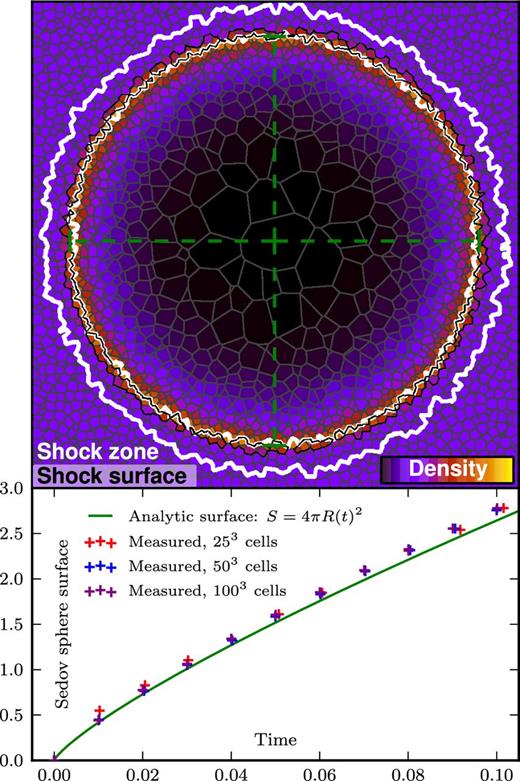
Top panel: cross-section of a three-dimensional Sedov blast wave simulation with 503 cells at t = 0.08 and energy E = 1. The colour map encodes the density field of the fluid, and the green dashed cross marks the analytically calculated extent of the Sedov blast wave at this time. The cells inside the white contours belong to the identified ‘shock zone’; they fulfil the three criteria described in Section 2.3.2. The black contours surround the cells that contain the reconstructed shock surface. These cells exhibit the minimum velocity divergence across the shock zone. Bottom panel: time evolution of the surface area of the spherical Sedov blast wave. We compare our approach to measure the shock surface in the test simulation (crosses) with the analytic evolution (solid line). For each cell in the shock surface, we assume an area contribution proportional to V2/3 with a pre-factor calibrated with shock tube simulations.
2.3.4 Mach number calculation
Given the pre- and post-shock values, the Mach number can in principle be calculated with any of the equations (1)–(4). Note however that the Mach number calculation with the entropy jump has to be accomplished with a numerical root finder, for example a Newton–Raphson method. In Section 3.2, we investigate the quality of the practical results achieved with each of these Mach number determination methods and conclude that the temperature jump is best suited for the computation of the Mach number in arepo, see also Fig. 2.
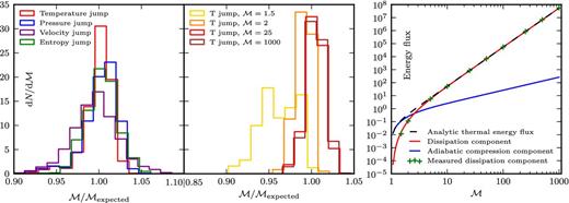
Left-hand panel: number of shock surface cells N per Mach number bin for 10 different shock tube tests (see Table 1) for different calculation methods of the Mach number. We obtain the best results for the temperature jump of equation (3). Middle panel: Mach number distributions of single shock tubes obtained with the temperature jump method. Low Mach numbers such as |$\mathcal {M}\simeq 1.5$| are slightly underestimated due to mild post-shock oscillations. This effect vanishes for Mach numbers |$\mathcal {M}\ge 2$|, where the correct value is found with an accuracy of 1 per cent. In both the left-hand and middle panels, each histogram is normalized such that the area under the curve is unity. Right-hand panel: thermal energy fluxes in shock tubes, separately for the adiabatic and dissipative components. We compare the measurement using the temperature jump with the analytic solution, finding excellent agreement.
2.4 Energy dissipation
Note that equations (8) and (9) describe the thermalization efficiency at shocks without considering cosmic rays. The possibility of cosmic ray acceleration and the corresponding efficiencies are addressed in Section 4.7.
3 VALIDATION
3.1 Sedov–Taylor blast wave
We test the determination of the shock surface with simulations of three-dimensional point explosions. We performed runs with 253, 503, and 1003 cells. In order to obtain an unstructured Voronoi mesh free of any preferred directions for the initial conditions, we distribute mesh-generating particles randomly in the unit box (x, y, z) ∈ [0, 1]3. The mesh is then relaxed via Lloyd's algorithm (Lloyd 1982) such that a glass-like configuration is obtained. We then set up the initial conditions as follows: the whole box is filled with uniform gas of density ρ1 = 1 and pressure p = 10−4, the initial velocities are zero, and the adiabatic index is set to γ = 5/3. The energy E = 1 is injected into a single central cell of the grid.
We show a cross-section of the 503 simulation at t = 0.08 in the top panel of Fig. 1. At the corners of the box the initial glass-like grid is still visible. Note however that the cross-section of a three-dimensional Voronoi grid is in general no longer a Voronoi tessellation itself. The colour of the cells represents the density field of the fluid. The cells inside the white contours constitute the identified shock zone. The shock surface consists of the cells inside the black contour lines and features a position that agrees well with the expected position (extent of the green cross).
Determining the correct shock surface area is important for calculating the energy dissipation accurately. We describe in Section 3.2 how we measure this area from the shock surface cells. In the bottom panel of Fig. 1 we compare the time evolution of the measured surface area of the Sedov shock sphere with the analytic solution, which is given by S(t) = 4πR2(t) (green line), where R(t) = β(Et2/ρ1)1/5 (Landau & Lifshitz 1966). The coefficient β can be calculated numerically. We obtain the value β = 1.152 for γ = 5/3 from the code provided in Kamm & Timmes (2007). Our measurement tracks the expected scaling well but shows a small systematic overestimation of ∼5 per cent. We suspect the primary cause of the offset does not lie in the shock surface estimation itself but rather appears because the simulated blast wave is slightly ahead of the analytic solution due to low resolution present at early times (Springel 2010) in this self-similar problem.
3.2 Shock tubes
We also checked the accuracy of the Mach number estimate for the identified shock surface by performing numerous shock tube tests (Sod 1978). In view of our target applications, we chose to adopt a three-dimensional box (x, y, z) ∈ [0, 100] × [0, 20] × [0, 20] in all the tests. Again, a hydrodynamic glass-like initial grid is used with 4 × 10⁴ cells. The gas has an adiabatic index of γ = 5/3, and the initial position of the discontinuity is prepared at x = 50. The variables of the right state (x > 50) are set to pr = 0.1, ρr = 0.125, and vr = 0. The density and the velocity of the left state (x < 50) are ρl = 1 and vl = 0, respectively. Furthermore, we assign a pressure pl to the left state such that the shock has a specific Mach number, see Table 1. The third column of the table shows the simulation time at which the shock reaches x = 75. We apply our shock finder to the corresponding output file. Note that the shock finder in this test, in contrast to the Sedov–Taylor blast wave, is also confronted with rarefaction waves and contact discontinuities, which obviously should not be mistaken as shock features by the shock finder.
Shock tube initial conditions. The pressure of the left state (pl) is varied such that the shock has a specific Mach number. The right-hand column indicates the time tend when the shock has traversed three quarters of the tube, at which point we measure its strength with our shock finder implementation.
| pl | |$\mathcal {M}$| | tend |
|---|---|---|
| 0.81445190 | 1.5 | 14.43 |
| 1.9083018 | 2.0 | 10.83 |
| 15.357679 | 5.0 | 4.330 |
| 63.498622 | 10.0 | 2.165 |
| 400.51500 | 25.0 | 0.8660 |
| 1604.1492 | 50.0 | 0.4330 |
| 6418.6865 | 100.0 | 0.2165 |
| 40 120.448 | 250.0 | 0.08660 |
| 160 483.88 | 500.0 | 0.04330 |
| 641 937.62 | 1000.0 | 0.02165 |
The left-hand panel of Fig. 2 shows the quality of the Mach number determination for all considered Mach number calculation methods according to equations (1)–(4), except for the density jump method which is omitted because it is not sensitive for high Mach numbers because ρ2/ρ1 → (γ + 1)/(γ − 1) for |$\mathcal {M}\rightarrow \infty$|. We note that in order to apply the velocity jump method, the velocities have to be transformed into the lab frame (Vazza et al. 2009).
The overall best results with arepo for the shock tube tests are obtained with the temperature jump method according to equation (3). It performs very well for Mach numbers |$\mathcal {M}\ge 2$|, as can be seen in the middle panel of Fig. 2. For small Mach numbers (|$\mathcal {M}<2$|), there are mild post-shock oscillations which cause the temperature jump method to underestimate the Mach number by a few per cent. This systematic offset is present for all jump methods, unless the entropy jump is used, which is not perturbed by these adiabatic oscillations.
For calculating the energy dissipation, the correct shock surface area has to be determined. The area contribution Si of a single cell to the whole shock surface is expected to scale with its volume according to |$V^{2/3}_i$|. Furthermore, Si also depends on the shape of the cell. Cells in a shock are compressed normal to the shock direction and the degree of the compression depends on the strength of the shock. We therefore make the ansatz |$S_i=\alpha F_i^\beta V^{2/3}_i$|, where Fi is the maximum face angle of the Voronoi cell, which characterizes the shape of the cell. The definition of this quantity has been introduced in Vogelsberger et al. (2012) in the context of a mesh regularization switch. We calibrate the constants α and β with a least-square fit using the 10 shock tube problems described above, where the total area of the shock surface is expected to be equal to the cross-section of the tube (S = 400). Our calibration yields α = 1.074 and β = 0.4378. By using these values, we obtain for the mean shock surface area of the tubes <S > = 396.35 ± 2.45, which is accurate to within 1 per cent. Note that in Fig. 1 we have demonstrated that also curved shock surfaces are measured to high accuracy.
With accurate Mach numbers combined with accurate shock surface areas in each shocked cell, we are able to calculate the dissipated energy on a cell-by-cell basis. We show this explicitly in the right-hand panel of Fig. 2. The shock finder measures the dissipative component of the thermal energy flux across a shock surface. The second component contributing to the total thermal energy flux is given by the adiabatic compression, which is present behind the shock. As can be seen from the figure, the adiabatic thermal energy flux is only relevant for small Mach numbers (|$\mathcal {M}\le 5$|).
4 SHOCKS IN NON-RADIATIVE SIMULATIONS
4.1 Simulation set-up
Besides full physics runs, the Illustris simulation suite (Genel et al. 2014; Vogelsberger et al. 2014a,b) contains also dark matter only as well as non-radiative runs. In this work we investigate shocks in the non-radiative runs, which include dark matter as well as gas, but no radiative cooling, star formation, and feedback. The cosmological parameters are consistent with the 9-year Wilkinson Microwave Anisotropy Probe (WMAP9) measurements (Hinshaw et al. 2013), and are given by Ωm = 0.2726, ΩΛ = 0.7274, Ωb = 0.0456, σ8 = 0.809, ns = 0.963, and H0 = 100 h km s−1 Mpc−1 with h = 0.704. Two simulations with a resolution of 2 × 4553 and 2 × 9103 were carried out in a periodic box having 75 h−1 Mpc on a side, where the factor of 2 indicates that the same number of gas and dark matter elements were used. The adiabatic index of the gas is set to γ = 5/3. In the following, we refer to these runs as Illustris-NR-3 and Illustris-NR-2, where the latter is the one with the higher resolution. The corresponding dark matter mass resolutions are 4.008 × 10⁸ and 5.010 × 10⁷ M⊙; the gas mass resolutions are kept fixed within a factor of 2 at 8.052 × 10⁷ and 1.007 × 10⁷ M⊙ (‘target gas mass’) by the quasi-Lagrangian nature as well as the refinement and derefinement scheme of arepo. For redshifts z > 1, the gravitational softening lengths of all mass components are equal and constant in comoving units, growing in physical units to 2840 and 1420 pc at z = 1 for the NR-3 and NR-2 run, respectively. For z ≤ 1, the softening lengths of the baryonic mass components are kept fixed at these values.
4.2 Shock finder assessment
The comparison with the shock finder measurement is shown in the top panel of Fig. 3. We find that our shock finder recovers the full amount of dissipated energy for low redshifts within 15 per cent accuracy. For very high redshifts, a progressively larger deviation occurs and our shock detection results do not account for all the dissipated energy any more. The origin of this difference lies in the topology of early shocks, which are not yet pronounced and resolved well at high redshift. Instead, they are rather scattered and occupy a large fraction of the simulation volume. As can be seen in the bottom panel of Fig. 3, the deviation kicks in at progressively higher redshift for higher resolution simulations. We hence conclude that our shock finder statistics has an effective redshift completeness limit which depends on the resolution. We can trust the shock detection results from z = 0 up to z ≈ 4.0 or z ≈ 5.0 for the Illustris-NR-3 or Illustris-NR-2 runs, respectively.
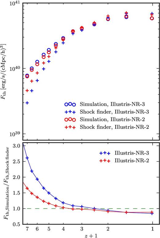
Comparison between the total energy dissipation rate found either with the shock finder, or inferred from two consecutive time-steps of a non-radiative simulation. The absolute values are shown in the top panel, the ratio is given in the bottom panel. We find fairly good agreement for low redshifts, indicating that our shock finder properly accounts for all significant shock dissipation in the simulation. However, at high redshift not all the shock dissipation is recovered by the shock finder, an effect that diminishes greatly with better numerical resolution.
4.3 Reionization modelling
The simulations Illustris-NR-3 and Illustris-NR-2 have no significant temperature floor and do not model cosmic reionization during their runtime. However, it is important to account for the nearly uniform heating of the ambient gas at the reionization redshift (z ≃ 6–7) in order to avoid overestimating the Mach numbers of shocks from voids onto filaments at late times. For this purpose, we use a temperature floor of 104 K for the shock finding carried out in post-processing, the same procedure as used by Ryu et al. (2003) and Skillman et al. (2008). We can justify the simplicity of this approach by the marginal contribution made by shocks with low pre-shock temperature and density (voids onto filaments) to the dissipated energy, which is the main quantity of interest in our analysis. Nevertheless, reionization in post-processing could of course be modelled in a more sophisticated way, for example by a fitting function in the density–temperature plane (Vazza et al. 2009).
4.4 General properties
In Fig. 4 we present the state of the Illustris-NR-2 simulation at redshift z = 0. The projections were created by means of point sampling, and the shown quantities are the mass-weighted temperature, the mean baryonic overdensity, the Mach number weighted with the dissipated energy, and the mean dissipated energy density. The latter two are displayed only for the top left-hand quarter of the former projections, which show a supercluster including the biggest halo of the simulation. This halo has a mass of M200, cr = 3.2 × 10¹⁴ M⊙, corresponding to a virial radius of r200, cr = 1.4 Mpc.
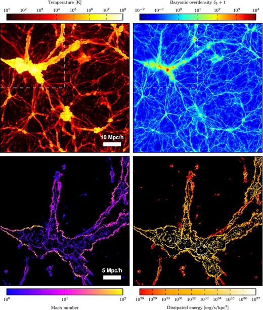
Top panels: projections of the mass-weighted temperature and mean baryonic overdensity of the Illustris-NR-2 run at redshift z = 0. The width and the height of the plots correspond to the full box size (75 h−1 Mpc). The projection in the z-direction has a depth of 150 kpc and is centred onto the biggest halo in the simulation. Bottom panels: Mach number field weighted with the energy dissipation and mean energy dissipation rate density for the top left-hand quarter of the box. Strong external shocks with Mach numbers up to |$\mathcal {M}\sim 100$| onto the supercluster are visible, as well as mostly weak shocks in the interior. However, most of the energy gets dissipated internally due to the higher pre-shock density and temperature. Note that we do not find many shocks inside the accretion shock onto the biggest halo, because here the gas motion is governed by subsonic turbulence, see also Fig. 7.
Note that due to the temperature floor applied in post-processing only the hottest filaments are detected by the shock finder and are hence present in the bottom panels. We can clearly observe the well-known fact (Ryu et al. 2003) that high Mach numbers (|$\mathcal {M}\sim 10\hbox{-}100$|) are generated at external shocks involving pristine pre-shock gas (Tpre ≲ 104 K), whereas gas previously processed by internal shocks (Tpre > 104 K) experiences typically lower Mach numbers (|$\mathcal {M}\lesssim 10$|). The density inside the supercluster exceeds the density of the voids by several orders of magnitude and thus the energy dissipation is most effective internally. The highest dissipation rate in this projection is present in the accretion shock onto the biggest cluster, whereas we do not detect many shocks inside the accretion shock.
4.5 Shock statistics
Fig. 5 quantifies the shock distribution and the associated energy dissipation in the Illustris-NR-2 run. In the left-hand panel, the differential shock surface area normalized by the simulation volume is plotted as a function of the Mach number. We find redshift independently that 50 per cent of the shocks have Mach numbers below |$\mathcal {M}=3$|, and 75 per cent below |$\mathcal {M}=6$|. Towards lower redshift the cumulative area of shocks increases, especially for strong shocks. At redshift z = 6, shocks with a Mach number smaller than |$\mathcal {M}=12$| account for 99 per cent of all the shocks, whereas at z = 0 all the shocks up to |$\mathcal {M}=35$| make up 99 per cent. At low redshift, the accretion from previously unshocked gas onto hot filaments and cluster outskirts provides Mach numbers up to |$\mathcal {M}\approx 100$|. At redshift z = 0, the total shock surface area reaches a value of S = 2.5 × 10⁻¹ Mpc2/Mpc3 (integral of the blue curve).
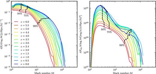
Left-hand panel: differential shock surface area as a function of Mach number for different redshifts. The black lines indicate the Mach numbers up to which a specific fraction of the total surface is included. Right-hand panel: distribution of the dissipated energy (generated thermal energy per time). We find that shocks with |$\mathcal {M}<6$| account for more than 75 per cent of all the shocks as well as 75 per cent of the total dissipated energy at all redshifts. Compared to former studies, the peak of our energy dissipation distribution at z = 0 is located at a considerable higher Mach number (|$\mathcal {M}\approx 2.7$| instead of |$\mathcal {M}\approx 2$|).
The right-hand panel of Fig. 5 shows the differential thermal energy flux as a function of the Mach number. The total dissipated energy increases with time up to z = 0.5 and drops thereafter slightly to a value of 2.3 × 1040 erg s−1 Mpc−3 (see also Fig. 3, but be aware of the factor h3). The increase in time is expected due to an increasing number of shocks and the ever higher pre-shock densities and temperatures found inside structures. At low redshifts, this effect saturates and, furthermore, dark energy slows structure growth and dilutes the pre-shock gas inside voids, which leads to a drop of the thermal energy flux for high Mach numbers. The latter observation has also been pointed out by Skillman et al. (2008).
We find that 50 per cent of the total energy dissipation occurs in shocks with |$\mathcal {M}<4$|, and 75 per cent in shocks with |$\mathcal {M}<6$|. Mach numbers above |$\mathcal {M}>40$| do not contribute significantly to the dissipation. We find that the energy dissipation peaks for z = 6 at |$\mathcal {M}\approx 2.3$| and shifts towards |$\mathcal {M}\approx 2.7$| for z = 0. This peak position at redshift zero differs considerably from the value |$\mathcal {M}\approx 2$| found by different previous studies (Ryu et al. 2003; Pfrommer et al. 2006; Skillman et al. 2008; Vazza et al. 2009, 2011). We believe that the origin of this discrepancy lies in the improved methodology we adopt, and we will elaborate more on this in Section 5.
Additional differences become apparent if we investigate the shock locations. In Fig. 6 we show the distribution of energy dissipation with respect to pre-shock densities (top panel) and pre-shock temperatures (bottom panel). Note however that this plot is not directly comparable to a similar investigation in Skillman et al. (2008) since their analysis is based on the inflowing kinetic energy. As expected, the relative contribution of shocks in the densest regions increases with time while shocks in low-density gas become less important. At redshift zero, 68 per cent of the energy dissipation is due to shocks with baryonic pre-shock overdensities 101 ≤ δb < 103. On the other hand, only 19 per cent of the dissipated energy heats cluster cores (δb ≥ 103).
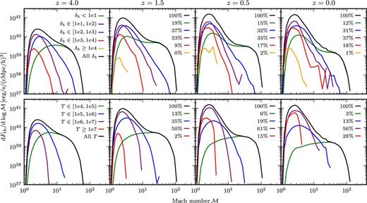
Contribution of different baryonic pre-shock overdensities (top panels) and pre-shock temperatures (bottom panels) to the overall energy dissipation in the Illustris-NR-2 run. We find that most of the energy dissipation at z = 0 is due to shocks with pre-shock overdensities in the range δb ∈ [101, 103). Furthermore, around 70 per cent of the total dissipation is contributed by pre-shock gas with temperatures T ∈ [105, 107), of which most is located in the WHIM.
The temperature contributions show the typical bimodal distribution consisting of external and internal shocks (Ryu et al. 2003). Previously unshocked cold gas accretes in strong external shocks but accounts only for a small amount of the dissipated energy. On the other hand, gas which gets shocked multiple times and is thus located inside structures produces low Mach number shocks with high energy dissipation. At redshift zero, gas with pre-shock temperatures 105 ≤ T < 107 accounts for 69 per cent of the energy dissipation. Moreover, in order to determine the contribution of the WHIM, we examine the density of the gas in this pre-shock temperature range and find that ≈54 per cent has a baryonic overdensity below δb = 100. A detailed breakup of the dissipation rates in different bins of pre-shock density and temperature is given in Table 2.
Contributions to the total energy dissipation for different pre-shock temperature and baryonic overdensity ranges at redshift z = 0. We find that ≈38 per cent of the energy gets dissipated by pre-shock gas of the WHIM (T ∈ [105, 107), δb < 102), and ≈57 per cent of the thermalization happens in clusters and groups (δb ≥ 102).
| Temperature range (in K) | ||||
|---|---|---|---|---|
| [104, 105) | [105, 106) | [106, 107) | [107, ∞) | |
| δb < 101 | 2 per cent | 4 per cent | 6 per cent | 0 per cent |
| δb ∈ [101, 102) | 1 per cent | 6 per cent | 22 per cent | 3 per cent |
| δb ∈ [102, 103) | 0 per cent | 2 per cent | 20 per cent | 15 per cent |
| δb ∈ [103, 104) | 0 per cent | 1 per cent | 7 per cent | 10 per cent |
| δb ≥ 104 | 0 per cent | 0 per cent | 1 per cent | 1 per cent |
We interpret our findings as follows. Almost 40 per cent of the thermalization happens when gas from the WHIM gets shock heated, whereas shocks inside the accretion shocks of clusters and groups (δb > 100) account for ≈60 per cent of the dissipation. Thus, the relative importance of the WHIM is significantly higher than what has been found in previous studies. Furthermore, the shocks we identify in clusters and groups are prominent merger shocks rather than stemming from halo-filling, complex flow patterns, as shown in the next section.
4.6 Galaxy cluster shocks
Fig. 7 shows zoom projections of width 100 kpc around different massive haloes of the Illustris-NR-2 simulation. The eight chosen haloes are sorted by mass, and we show the baryonic overdensity as well as the energy dissipation by shocks. The white circle indicates the virial radius r200, cr. The first halo is the biggest halo in the simulation and is also present in Fig. 4. As can be seen in the gas projection, there are turbulent motions inside the virial radius. However, we do not find many shocks inside this region, which points towards predominantly subsonic turbulence.
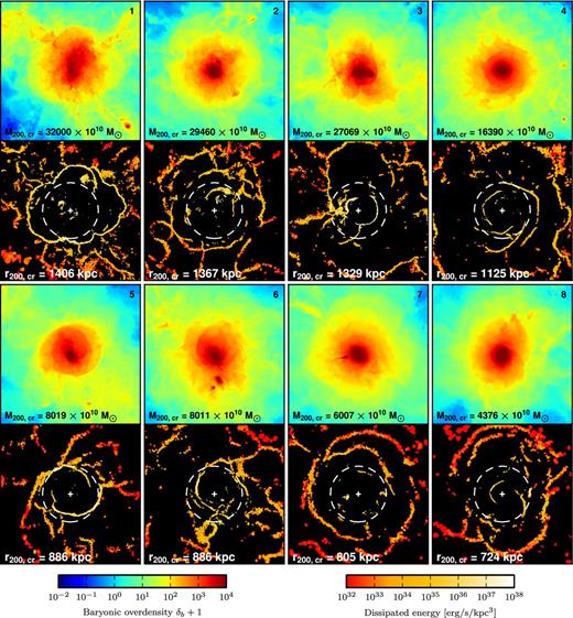
Zoom projections with a width of 100 kpc centred on some of the biggest haloes in the Illustris-NR-2 simulation. The top panels show the baryonic overdensity while the bottom panels indicate the energy dissipation. Accretion shocks onto the haloes can be found close to but outside of r200, cr (white circles). Inside the accretion shocks prominent merger shocks are present. We do not find many shocks due to complex flow patterns within clusters, unlike reported by previous studies.
The third halo is in a state similar to the bullet cluster. The small subcluster ploughs through the gas of the big halo and produces a bow shock where a lot of energy is dissipated. The Mach number along the bow shock is |$2\lesssim \mathcal {M}\lesssim 3.5$|, comparable to the value |$\mathcal {M}=3\pm 0.4$| measured for the bullet cluster system (Markevitch et al. 2002; Markevitch 2006). The shocks in haloes four and five form interesting spiral structures. These shocks might point towards the following scenario: a minor-merger event triggers gas sloshing and the formation of a spiral cold front (Ascasibar & Markevitch 2006; Markevitch & Vikhlinin 2007; Roediger & Zuhone 2012) which steepens to a shock while propagating outwards. A hint could also be the temperature map of halo four, which indicates that the spiral shock structures fade into contact discontinuities in the interior. In halo six, there are fine shock structures close to each other. In order to resolve these, it is crucial to handle overlapping shock zones as described in Section 2.3.3. The last two haloes are surrounded by prominent accretion shocks. Furthermore, halo eight underwent a merger event recently, as can be seen from the shock remnants inside the virial radius lying opposite to each other. Several of such remnants have been observed in form of double radio relics, as reported for example in Rottgering et al. (1997), Bonafede et al. (2009, 2012), and van Weeren et al. (2009). The accretion shocks are located outside of the virial radius r200, cr. This is expected since the kinetic and thermal pressure become roughly equal around r200, mean (Battaglia et al. 2012) which is ≈1.5 r200, cr at redshift z = 0.
In Fig. 8, we present the radial shock distribution for several of the haloes of Fig. 7. For the biggest halo in the simulation (halo 1, red curve) the accretion shock is located at around 1.6 r200, cr. The green curve (halo 3) shows the bow shock of the bullet at approximately 0.6 r200, cr, however, no single radius for the accretion shock can be determined for this highly dynamical system. In the blue curve (halo 8) three bumps can be seen. The first one corresponds to the merger shocks inside the virial radius (R = 0.4). The two bumps outside the virial radius belong both to the accretion shock and are located at the minor (R = 1.2) and major axis (R ≈ 1.9) of the projected accretion shock ellipsoid. In order to estimate an average radius for accretion shocks, we stack the distributions of the 1000 largest haloes in the simulation (1.7 × 10¹² M⊙ ≤ M200, cr ≤ 3.2 × 10¹⁴ M⊙) and average them (black curve). We find a signal with a broad peak at R = 1.3, implying that the accretion shocks at redshift z = 0 can typically be found at around 1.3 r200, cr.
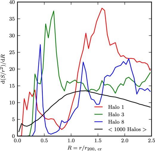
The radial shock surface distribution in several of the haloes of Fig. 7 (coloured lines, as labelled) as well as the average distribution of the 1000 largest haloes in the Illustris-NR-2 simulation, stacked at redshift z = 0. The average dissipation profile has a peak at around R = 1.3 in units of the virial radius, which can be interpreted as the typical radius of the accretion shocks.
4.7 Cosmic ray acceleration
In this section, we discuss the role of the detected shocks in the Illustris-NR-2 run as cosmic ray sources. While our analysis is carried out by post-processing simulation outputs, cosmological simulations including cosmic rays and associated processes have also been presented, for example in Miniati et al. (2001), Pfrommer et al. (2007), Jubelgas et al. (2008), and Vazza et al. (2012).
Cosmic rays get injected in collisionless cosmological shocks by means of the DSA mechanism (e.g. Blandford & Ostriker 1978; Malkov & O'C Drury 2001), also known as first-order Fermi acceleration. In this process, ions with high thermal energies can diffuse upstream after crossing a shock and gain in a repetitive way in multiple shock crossings more and more energy. The cosmic ray injection efficiency depends strongly on the Mach number as well as on the level of Alfvén turbulence, and is most efficient if the magnetic field is parallel to the shock normal. Simulations of this DSA scenario were carried out by Kang et al. (2007), inferring upper limits for the cosmic ray acceleration efficiency at specific Mach numbers, in the case of a pre-existing as well as a non-pre-existing cosmic ray population. Furthermore, fitting functions η(M) are provided for both cases and we use these for estimating the energy flux |$f_{\rm CR}=\eta (M)f_\Phi$| transferred into cosmic rays, where |$f_\Phi$| is the processed kinetic energy flux.
The kinetic energy processed by shocks in the simulation as well as the estimated available energies for cosmic ray acceleration at redshift z = 0 are presented in the top panel of Fig. 9. The total inflowing kinetic energy amounts to 1.14 × 1041 erg s−1 Mpc−3. Without a pre-existing cosmic ray population most of the acceleration energy is available in shocks with Mach numbers M ≈ 3.2 (blue curve). Furthermore, if we compare the integrals of the distributions, we estimate that ≈6 per cent of the total kinetic energy processed by shocks is transferred into cosmic rays. In the case of pre-existing cosmic rays, which are generated in shocks at earlier times, the DSA mechanism is more efficient, especially for low Mach numbers (red curve). For this scenario, we find a peak position at M ≈ 2.5 and a kinetic energy transfer to cosmic rays amounting to ≈18 per cent.

Top panel: Mach-number-dependent energy distribution for accelerating cosmic rays according to the DSA simulations of Kang et al. (2007). The black line shows the total kinetic energy processed by shocks per time and volume, while the red and blue curves give the fractions expected for particle acceleration with and without pre-existing cosmic rays, respectively. Bottom panel: contribution of different baryonic pre-shock overdensities to the total energy used for cosmic ray acceleration.
In order to determine the spatial origin of the cosmic rays, we show the contributions of different baryonic overdensities to the total cosmic ray energy in the bottom panel of Fig. 9. For both scenarios (with and without pre-existing cosmic rays) most of the energy transfer into cosmic rays is located in regions with densities 10 ≤ δb < 103 (≈68 per cent). Without a pre-existing population, only 43 per cent of the cosmic ray energy is generated inside clusters and groups (δb > 100). On the other hand, pre-existing cosmic rays increase the efficiency for low Mach number shocks, which are mainly present inside dense structures. In this case we find that 58 per cent of the energy for cosmic ray acceleration is provided by shocks inside clusters. We conclude that cosmological shocks could produce a significant amount of cosmic rays. Furthermore, the relevant shocks are shared in comparable proportions among both, regions with overdensities above and below δb = 100.
5 METHODOLOGY VARIATIONS
In this section, we turn to an investigation of the origin of the discrepancies between our results and previous studies. For this purpose, we in particular investigate the shock zone determination criteria as well as the Mach number calculation approach for shock detection in the Illustris-NR-2 run.
For calculating the Mach number of shock surface cells, we normally evaluate pre- and post-shock temperatures of cells just outside the shock zone. An exception to this are overlapping shock zones, in which case the pre-shock temperature is taken inside the combined shock zone and between the shock surfaces. Note that with this procedure, Mach numbers are calculated across a variable number of cells (variable jump range), depending on the extent of the imprint of the shock on the primitive variables. In Fig. 10 we show how the inflowing kinetic energy distribution as well as the dissipated energy distribution changes when we adopt a fixed jump range instead by calculating the Mach number always from the directly adjacent cells of a shock centre (short jump). Both distributions are shifted towards slightly lower Mach numbers. This finding is expected since a short jump does not fully enclose the broadened shock, and should hence lead to a smaller jump in the measured temperatures. For the dissipated energy distribution we find a peak shift from |$\mathcal {M}\approx 2.7$| to ≈2.2 as well as a reduction of the total dissipated energy by ≈15 per cent when the short jump is adopted.
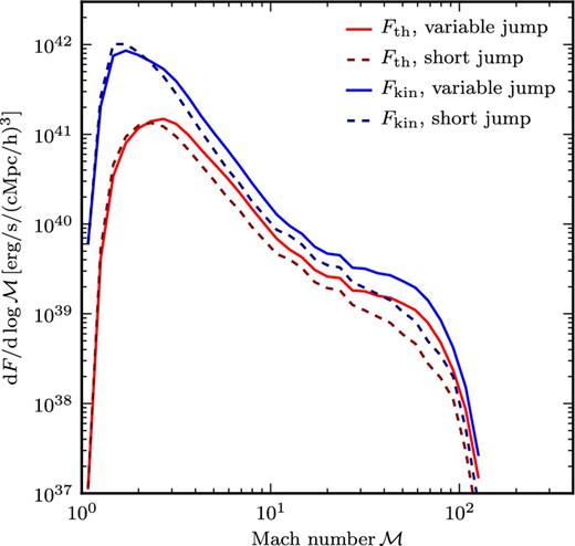
Effect on the inflowing kinetic energy and dissipated energy when we calculate the Mach number based just on neighbouring cells (short jump) instead of using our standard implementation with a variable jump range. The restriction to short jumps shifts the distributions to slightly lower Mach numbers.
In the next test we compare our default implementation of shock zone finding to a method in which the requirement for a minimum pressure jump (|$\Delta \log p\ge \log \left. p_2/p_1\right|_{\mathcal {M}=\mathcal {M}_{{\rm min}}}$|) is abandoned, and the criterion ∇T · ∇ρ > 0 is replaced with ∇T · ∇S > 0. These relaxed criteria have been frequently used in previous studies and only recently Hong et al. (2014) suggested a replacement of the temperature–entropy criterion.
In Fig. 11, we visualize the differences by applying the two methods to the Illustris-NR-2 simulation, omitting a temperature floor here for the purposes of this comparison test. With the old standard shock finding method (right-hand panel), many more low Mach number shocks are found inside the WHIM and inside galaxy clusters. The additional shocks increase the total energy dissipation and the relative contribution of clusters due to high pre-shock densities and temperatures.
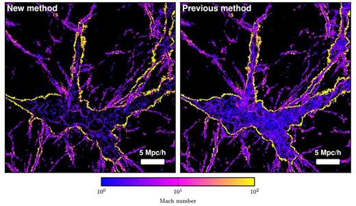
Demonstration of the difference between our default shock finder implementation (left-hand panel) and the old standard method (right-hand panel). With the latter implementation many more shocks are found inside the WHIM and inside clusters. These shocks are spurious as demonstrated in Fig. 12. Depending on the applied evaluation method for the shock strength, some of the spurious shocks can be suppressed as shown in Fig. 13. Nevertheless, if spurious shocks enter the analysis the relative contribution of clusters to the total dissipated energy is overestimated. Note that for this comparison we do not adopt a temperature floor and thus find more shocks and higher Mach numbers compared to Fig. 4.
We demonstrate in Fig. 12 that the additional shocks are spurious by applying the old method to a three-dimensional Kelvin–Helmholtz simulation in which no shocks are present. However, the old implementation is not able to filter tangential and contact discontinuities reliably in the shock zone determination, and thus false positive shocks are found along the density jump.
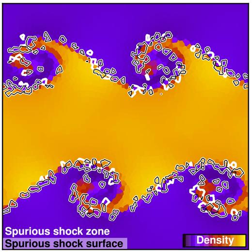
Application of the previous standard shock finding method to a three-dimensional Kelvin–Helmholtz instability simulation. This method does not filter tangential and contact discontinuities and thus finds spurious shocks even though this subsonic problem is formally free of shocks. Our new implementation on the other hand does not find shocked cells at all in the simulation volume, as desired.
Depending on the applied scheme for assessing the shock strength (temperature jump, density jump, or velocity jump), some of the spurious shock detections are suppressed by the consistency check that requires a correct jump direction in the shock surface determination (Section 2.3.3). The energy dissipation inferred for the different methods and different jump evaluations is presented in Fig. 13. Note that the reionization model through a temperature floor is disabled here, and we therefore obtain a tail towards very high Mach numbers. It can be seen that the old standard shock finding method is very sensitive to the adopted jump quantity for inferring the Mach number, while our new method is rather stable. There is good agreement between the temperature jump and velocity jump methods, whereas the pressure jump evaluation shifts the Mach numbers towards higher values for very strong shocks.
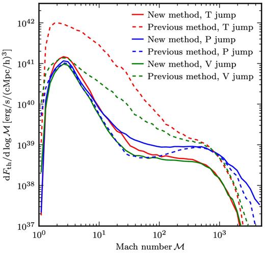
Comparison of our new method to a previous standard method which has no minimum pressure jump requirement and uses ∇T · ∇S > 0 instead of ∇T · ∇ρ > 0 as a shock zone criterion. The previous method does not filter tangential discontinuities in this case, see also Fig. 12. We furthermore investigate the dependence of these methods on the Mach number estimation by using instead of the temperature jump (our standard approach) also the pressure and velocity jumps, as labelled in the panel.
The old standard method in combination with the temperature jump gives clearly wrong results that are associated with an overestimate of the energy dissipation, which can be clearly seen from the difference of the dashed and the solid red line. By using the velocity jump instead, spurious shocks can be removed if the jump direction of the normal velocities is not consistent with the shock direction (temperature gradient). However, there remain then still a significant number of cases with wrong shock detections, both with low and high Mach numbers (green dashed line). Note that the pressure jump across such spurious shocks is very small such that only a small Mach number is assigned if the pressure discontinuity is used to measure the shock strength. However, the distribution of energy dissipation at high Mach numbers is also altered compared to our new method, and perhaps surprisingly it is lower in this case (blue dashed line). The origin of this effect lies in the modification of the Mach number of real shocks by spurious shocks. This happens whenever the shock zone of a real shock gets modified (extended) by the shock zone of a spuriously detected shock nearby.
We conclude that the use of a variable jump range gives a small improvement compared to a fixed small jump range. It is yet more important to properly filter against tangential and contact discontinuities already in the shock zone determination to robustly avoid spurious shock detections and distortions in the resulting shock statistics.
6 SUMMARY
We have implemented a parallel shock finder for the unstructured moving-mesh code arepo, based on ideas of previous work (Ryu et al. 2003; Skillman et al. 2008; Hong et al. 2014) combined with new refinements. Shocks are detected in a two-step procedure. First, a broad shock zone is determined by analysing local quantities of the Voronoi cells to identify regions of compression. In a second step, a shock surface is identified by finding cells with the maximum compression across the shock zone, followed by an estimate of the Mach number through measuring the temperature jump across the shock zone. In this way, the Mach number is calculated over a variable number of cells which adjusts to the numerical broadening of the particular shock.
Improvements to previous methods have been realized by handling overlapping shock zones and by carefully filtering out tangential discontinuities and contacts in the shock zone determination. Such discontinuities are abundantly present in cosmological simulations, for example in the form of cold fronts and in shear flows that mix gas of different specific entropy. We robustly suppress spurious shock detections by replacing the commonly used criterion ∇T · ∇S > 0 with ∇T · ∇ρ > 0 (as also adopted in Hong et al. 2014), and additionally by requiring a suitable minimum pressure jump threshold.
We have shown that shock finder results can be quite sensitive to implementation details. For example, allowing for a variable number of cells when evaluating the Mach number across shocks leads in general to slightly higher (and more correct) values compared to adopting a fixed number of cells. A still more important role is played by the choice of fluid quantities selected for the Mach number calculation. Especially when tangential and contact discontinuities are not cleanly filtered out, an unfortunate choice can here produce substantial distortions in the inferred shock statistics.
We have introduced a new test for assessing the overall performance of a shock finder in which the energy dissipation inferred from the shock detection is directly compared with the actual energy dissipation in a non-radiative cosmological simulation between two consecutive time steps. We find a good performance of our techniques for low redshifts z ≲ 4.0–5.0 in non-radiative cosmological simulations, where we can identify all strong shocks reliably and account accurately and in a numerically converged way for the bulk of significant dissipation in shocks. At zero redshift, the energy dissipation measured with our shock finder for the adopted cosmological parameters is measured to be 2.3 × 1040 erg s−1 Mpc−3.
Interestingly, we detected rich shock morphologies in the high-resolution non-radiative simulation Illustris-NR-2. In particular, high Mach number accretion shocks onto filaments and cluster outskirts nicely trace the cosmic web. Accretion shocks onto galaxy clusters dissipate a lot of energy, while merger shocks inside the clusters give hints about their recent formation history. We note that the merger shocks appear as rather prominent and distinct features, whereas we do not find complex flow shock patterns inside the cluster accretion shocks, suggesting that there the gas dynamics is mostly characterized by subsonic turbulence (which we expect to be well captured by arepo; Bauer & Springel 2012).
With our improved methodology, we find quantitatively revised results for the shock dissipation statistics in non-radiative cosmological simulations. Most of the thermalization happens in shocks with Mach numbers around |$\mathcal {M}\approx 2.7$|. Moreover, almost 40 per cent is contributed by shocks in the WHIM and ≈60 per cent by shocks in clusters and groups. Compared to previous studies, these findings correspond to a shift in the energy dissipation spectrum towards higher Mach numbers and towards structures with lower densities. Also, we have found R = 1.3 r200, cr as a typical radius for accretion shocks onto galaxy clusters at redshift z = 0, based on identifying a peak when stacking the radial shock dissipation profiles of 1000 haloes of the Illustris-NR-2 simulation. Consequently, the accretion shock is expected to typically lie slightly outside the virial radius, a finding which is consistent with Battaglia et al. (2012). We note however that the accretion shock position shows a high degree of temporal variability in any given halo.
Finally, we also investigated the expected energy transfer to cosmic rays in the identified large-scale structure shocks if acceleration efficiencies derived from DSA plasma simulations are adopted (Kang et al. 2007). These simulations are set up with a magnetic field parallel to the shock normal direction and provide therefore upper limits for the acceleration efficiency. We obtain at redshift z = 0 an average cosmic ray energy injection rate of 7.0 × 1039 erg s−1 Mpc−3 in the case of non-pre-existing cosmic ray populations, and a considerably larger value in the case of pre-existing cosmic rays. Considering these numbers, it is quite plausible that even for random magnetic field orientations a dynamically important cosmic ray population is produced in these shocks. Furthermore, we found that gas with pre-shock overdensities above and below δb = 100 contribute roughly equally to the energy transfer into cosmic rays.
In future work, it will be interesting to couple the shock finder to hydrodynamical simulations that take cosmic rays self-consistently into account. Also, it should be interesting to contrast the results obtained here for non-radiative simulations with an analysis of full physics simulations of galaxy formation that include radiative cooling and heating mechanisms, as well as prescriptions for star formation, stellar evolution, black hole growth, and associated feedback processes. These simulations feature interesting additional shocks, for example due to strong feedback-driven outflows. In a companion paper (in preparation), we will present an analysis of the corresponding shocks in the recent Illustris simulation (Vogelsberger et al. 2014a).
We thank Christoph Pfrommer, Rüdiger Pakmor, Andreas Bauer, and Shy Genel for very helpful discussions. The authors acknowledge financial support through subproject EXAMAG of the Priority Programme 1648 ‘SPPEXA’ of the German Science Foundation, and through the European Research Council through ERC-StG grant EXAGAL-308037.
