


Abstract
Numerical N-body simulations play a central role in the assessment of weak gravitational lensing statistics, residual systematics and error analysis. In this paper, we investigate and quantify the impact of finite simulation volume on weak lensing two- and four-point statistics. These finite support (FS) effects are modelled for several estimators, simulation box sizes and source redshifts, and validated against a new large suite of 500 N-body simulations. The comparison reveals that our theoretical model is accurate to better than 5 per cent for the shear correlation function ξ+(θ) and its error. We find that the most important quantities for FS modelling are the ratio between the measured angle θ and the angular size of the simulation box at the source redshift, θbox(zs), or the multipole equivalent ℓ/ℓbox(zs). When this ratio reaches 0.1, independently of the source redshift, the shear correlation function ξ+ is suppressed by 5, 10, 20 and 25 per cent for Lbox = 1000, 500, 250 and 147 h−1 Mpc, respectively. The same effect is observed in ξ−(θ), but at much larger angles. This has important consequences for cosmological analyses using N-body simulations and should not be overlooked. We propose simple semi-analytic correction strategies that account for shape noise and survey masks, generalizable to any weak lensing estimator. From the same simulation suite, we revisit the existing non-Gaussian covariance matrix calibration of the shear correlation function, and propose a new one based on the 9-year Wilkinson Microwave Anisotropy Probe)+baryon acoustic oscillations+supernova cosmology. Our calibration matrix is accurate at 20 per cent down to the arcminute scale, for source redshifts in the range 0 < z < 3, even for the far off-diagonal elements. We propose, for the first time, a parametrization for the full ξ− covariance matrix, also 20 per cent accurate for most elements.
INTRODUCTION
Weak gravitational lensing has emerged as one of the key methods to constrain astrophysical and cosmological parameters. The technique studies the distortions in the images of background luminous sources caused by foreground masses, and is therefore sensitive to the total matter content (dark matter, baryons and neutrinos) along and surrounding the photon's trajectories (see Munshi et al. 2008, for a review).
Recent results from the Canada–France–Hawaii Telescope (CFHT) Lensing Survey (CFHTLenS; Heymans et al. 2012; Erben et al. 2013) have shown the scientific potential of weak lensing in an environment where residual systematics are fully controlled. A non-exhaustive list of key results include accurate measurements of galaxy luminosity and stellar mass functions (Velander et al. 2014), studies of the galaxy/dark matter environmental connection (Gillis et al. 2013), tests for the laws of gravity (Simpson et al. 2013), large-scale structure mass maps (Van Waerbeke et al. 2013); it has also placed competitive constraints on many cosmological parameters (Fu et al. 2014), including the first tomographic analysis (Kilbinger et al. 2013), three-dimensional cosmic shear (Kitching et al. 2014) and mitigated the impact of intrinsic alignment of galaxies (Heymans et al. 2013). This is an impressive list of scientific results for a survey that is ‘only’ 150 deg2; the sky coverage from the upcoming analysis with the Red-Sequence Cluster Survey-2 (RCS2),1 Dark Energy Survey (DES),2 Kilo-Degree Survey (KiDS)3 and Hyper Suprime-Cam (HSC)4 surveys is more than an order of magnitude larger, therefore, significantly increasing the statistical precision.
Central to all weak lensing studies, mock galaxy catalogues, generally based on numerical simulations, are needed for the testing and calibration of statistical estimators. This is particularly important in the non-linear gravitational clustering regime, where theoretical predictions cannot be done analytically with high precision. Of equal importance is the necessity to understand any secondary signals (e.g. intrinsic alignment of galaxies, source–lens correlations) in a completely non-linear clustering environment. In addition, the accurate estimation of the sampling variance at small scale must be performed with numerical simulations. As shown in Heymans et al. (2012), this is an essential ingredient in the quantification of residual systematics, where random correlation of galaxy shapes with the telescope's point spread function cannot be neglected. An acute understanding of all these aspects is required for a reliable interpretation of the weak lensing data and an accurate treatment of its errors. While seeking to achieve these multiple goals, N-body simulations stand out as the best tool.
The first limitation of any ‘dark matter only’ calculation is that the results are known to be inaccurate at the galactic scales due to the absence of baryonic feedback. It was shown by Semboloni et al. (2011), van Daalen et al. (2014), Bird, Viel & Haehnelt (2012) that baryons and baryonic feedback can suppress the matter power spectrum by up to 20 per cents compared to a pure dark matter universe. The power suppression affects all scales differently, depending on a particular combination of active galactic nuclei, stellar winds and supernovae feedback. A similar trend also arises if neutrinos are allowed to be massive, contributing to an addition suppression of structure. Therefore, mock galaxy catalogues constructed from dark matter only simulations will overpredict the growth of structure at scales smaller than a megaparsec, by an amount that is largely unknown. In this work, we ignore the effect of baryons and massive neutrinos; these require another generation of hydrodynamical simulations, which are not available with the current computational resources.
The second limitation of numerical simulations is that they are performed inside a finite cosmological volume, therefore, density fluctuations larger than the computation box, also called ‘supermodes’, are completely ignored. Many studies have investigated how these supermodes impact the measurements of the matter power spectrum or the cosmic shear, but a full propagation on the cosmological parameter is not yet fully understood.
Covariance matrix: the state of affairs
In a finite volume simulation, the missing supermodes inevitably affect, via non-linear mode coupling, the clustering properties of dark matter in real space (Power & Knebe 2006) and in Fourier space (Smith et al. 2003; Takahashi et al. 2008; de Putter et al. 2012; Heitmann et al. 2014). In weak lensing simulations, the effect of missing supermodes propagates inside the extracted light cones, which yields to a suppression of power and variance over a large range of angular scales (Sato et al. 2009, 2011).
It seems useful at this point to recall that there are ways to measure covariance matrices other than from an ensemble of simulations. For instance, we can estimate the error from a single large realization – or from the data itself – by jackknife of bootstrap resampling subvolumes. This is not an ideal approach, and it was shown that such internal error estimates are biased by up to 40 per cent due to the residual correlations between the subvolumes (Norberg et al. 2009). Moreover, it requires a cosmological simulation that can achieve the angular resolution relevant for the science over a volume at least as large as the full survey. These are extremely challenging and expensive to run, especially if one is to meet the requirement of the upcoming weak lensing programmes. The MICE-Grand Challenge simulation (Fosalba et al. 2013), for instance, covers an octant on the sky, yet starting at θ = 27 arcmin (or ℓ ∼ 800) and for sources at zs = 1, it shows >10 per cent of loss in the cosmic shear two-point function due to resolution limitations. This is unfortunate since these small scales contribute significantly to the cosmic shear and galaxy–galaxy lensing signals, with exact proportions that depend on the estimator (in Kitching et al. 2014, it is shown that the sensitivity of the three-dimensional cosmic shear signal peaks at k ∼ 0.5 h Mpc−1 and spreads significantly up to k-modes well beyond unity). Even if the resolution could be improved in a next generation MICE-like effort, we would still rely on internal subsampling techniques to estimate the error, an approach that is only 40 per cent accurate.
Clearly, the precision requirements on the covariance matrix for upcoming and future weak lensing surveys, where both small and large scales have important weight, seem to demand an estimation based on ensembles of independent realizations. Running these is also computationally expensive and requires a careful trade-off between the number of realizations Nsim, the cosmological volume Lbox and the resolution. One the one hand, a good resolution is crucial in order to preserve the non-linear signature of the signal within acceptable limits. On the other hand, it was recently shown that a low Nsim has dramatic consequences (see Joachimi & Taylor 2014). As first pointed out by Hartlap, Simon & Schneider (2007), reducing the number of realizations inevitably leads to a noisy covariance matrix, and to a biased inverse matrix. It was then shown by Taylor, Joachimi & Kitching (2013) that it also leads to a larger error on the error bars. Finally, the noise in the covariance matrix contributes to an additional variance term on the cosmological parameters itself (Dodelson & Schneider 2013), which scales as (1 + Ndata/Nsim). Note that these calculations are only valid for independent realizations; for internal estimates of a single realization (i.e. with Nsim = 1), the extra variance term is currently unknown. In light of these results, Nsim should be at least as large as Ndata + 200 if one is to reach a 5 per cent error on cosmological parameters and keep the extra error under control. Given these constraints, the best strategy seems to involve a reduction of Lbox, while keeping high both the angular resolution and Nsim. Only then it is possible to correctly model the signal and minimize the extra error term, at the price of allowing finite box effects to contaminate our calculations. What matters then is to identify and keep track of all such effects, correcting those that can be corrected and accounting for any residual biases in the final error budget.
In the first part of the current paper, we therefore loosen the criteria on Lbox and investigate a novel consequence of the missing supermodes, which we refer to as the finite support (FS) effect. We verify our modelling of the FS effect and its correction against a new suite of N-body simulations, the Scinet Light Cone Simulations (SLICS) series, which intends to address the extra variance term discussed in the preceding paragraph. The SLICS contain a large ensemble (LE) with Nsim = 500, hence the extra error would be less than 10 per cent for a data vector of size Ndata < 50. It also contains a high resolution (HR) subsample that serves to assess the resolution of the LE suite.
While such weak lensing simulation suites can estimate the sampling covariance in the non-linear regime, they are computationally expensive to produce. As shown by Semboloni et al. (2007) and Sato et al. (2011), the results can be compressed into fit functions, which are portable and convenient for a number of cosmological applications such as forecasting or simple χ2 minimization. In the second part of this paper, we revisit the calibration of the covariance matrix about the cosmic shear two-point function5 ξ+, proposed by the authors above-mentioned, and suggest an improved parametrization based on the SLICS series. We also provide the first6 semi-analytical estimation of the non-Gaussian ξ− covariance matrix.
This paper is organized as follows. We start in Section 2 with a quick overview of the weak lensing theoretical modelling. In Section 4.6, we present general relations that describe the finite volume effects as a function of source redshift, angle and simulation box size. We validate these relations against N-body calculations in Section 4, in which we first present the numerical set-up of the SLICS. We then compare the measurements of cosmic shear two-point functions against predictions from three theoretical models, and validate our modelling of the FS effect. In Section 5, we turn our attention on the smaller angular scales and propose accurate parametrizations of the non-Gaussian estimators of the ξ± covariance matrices. In Section 6, we discuss the practical implementation of the FS correction in data analysis pipelines, in the presence of general source redshift distributions and survey masks. We conclude afterwards.
THEORETICAL BACKGROUND
We describe here the theoretical modelling of the weak lensing two-point functions, and explain how supermodes effects are incorporated in the predictions.
|$\boldsymbol {P(k)}$| – models
One of the drawbacks of the halofit approach is that it attempts to describe the non-linear coupling with a single fitting function; whether this can truly capture all the information is questionable. As an alternative, the Cosmic Emulator (CE; Heitmann et al. 2010, 2014) is based on an interpolation between a set of measurements from simulations, which were performed at carefully selected points in parameter space. In this paper, we thus consider the CE as a third model, and take advantage of the extended edition that achieves better than 5 per cent precision on the dark matter power spectrum up to k ∼ 10.0 h Mpc−1. It is constructed from 37 cosmologies, each sampled with nested N-body simulations of different volumes. The largest modes were assessed to be accurate to better than a per cent by comparing results with simulations of Lbox = 2 h−1 Gpc. In other words, the CE was explicitly shown to be minimally affected by the finite box effects under consideration in the current work, which ensures that the largest scales are fully reliable. Unfortunately, the scope of the excursion in parameter space is not as large as the halofit models, hence it might not be adequate for some analyses. There have been efforts in the past to stitch the halofit predictions on top of the CE in order to cover cosmological parameter and k-modes that are outside of the range of validity (Eifler 2011), but this falls outside the needs of the current paper.
|$\boldsymbol {C^{\kappa }_{\ell }}$| – models
Different prediction models considered in this paper. In most of the calculations, we use Lbox = 505 h−1 Mpc (or kbox = 0.0124 h Mpc−1). For the CE predictions only, the box size is allowed to vary to 1000, 505, 257 and 147 h−1 Mpc. We regroup all these volumes under the quantity Lvar, as indicated in this table. Note that both the CE and CEk models have kmax = 10.0 h Mpc−1, which is the resolution limit of the CE.
| Model | k-modes included | Name |
|---|---|---|
| (h Mpc−1) | ||
| halofit2011 | 0.0010 < k < 40.0 | HF1 |
| halofit2011+k-cuts | 0.0124 < k < 10.0 | HF1k |
| halofit2012 | 0.0010 < k < 40.0 | HF2 |
| halofit2012+k-cuts | 0.0124 < k < 10.0 | HF2k |
| CE | 0.0010 < k < 10.0 | CE |
| CE+k-cuts | 2π/Lvar < k < 10.0 | CEk |
|$\boldsymbol {\xi _{\pm }(\theta )}$| – models
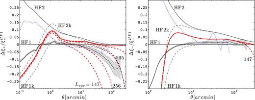
Fractional error on ξ+ (left) and ξ− (right) with respect to the halofit2011 predictions, for zs = 0.582. We show results from the two simulations suites (LE and HR) plus all models of Table 1. The cut at k = 0.0124 h Mpc−1 becomes important in ξ+, and all models converge to the same level of suppression (indicated by the label ‘505’ in the figure). For the CEk model (dashed red), four different values of Lvar are visible in the left-hand panel – 147, 256, 505 and 1000 h−1 Mpc, while only Lvar = 147 h−1 Mpc is seen in the right-hand panel. We note that the ξ+ (ξ−) models disagree significantly at scales close to 1.0 (10.0) arcmin.
The different ξ+(θ) models (left-hand panel) with no k cuts agree within less than 5 per cent at scale larger than 10 arcmin. The cut-off of modes with k > 10.0 h Mpc−1 results in a sharp turn over at scales just under the arcminute for all models, suggesting that data analyse involving larger angular scales (zs ≥ 0.6) could rely on the CE (thick red) as an alternative (or a cross-check) to halofit. The HF2 predictions (solid upper black line) is consistently higher than the CE by about 3–5 per cent. This cut-off also produces a small bump at the turnover scale of 1 arcmin, as seen in the two halofit predictions HF1k and HF2k (black dashed lines). This is a numerical effect due to the interaction between a sharp cut-off and the oscillatory J0 function. It is likely that in absence of the built-in high-k cut, the CE model would be lower by about 2–3 per cent at the turnaround scale. Overall, the differences between the models below 1 arcmin are large, and this source of theoretical uncertainty will have to be addressed in weak lensing analyses involving these scales. Note that this is also a scale where the baryonic effects are very important.
A striking feature seen in the left-hand panel of Fig. 1 is the impact of the low-k (large scale) cut. In all three models, excluding the k < 2π/505 h Mpc− 1 modes produce a significant suppression of power, of 1 per cent for θ ∼ 10 arcmin, 5 per cent by a degree and by more than 10 per cent for θ > 2° (see the dashed line labelled ‘505’). The other thick red dashed lines in the figure show the CEk predictions for different box sizes. Other models behave the same way. As expected, the smaller the box, the larger the effect. Even the 1 Gpc h−1 box prediction suffers from a 5 per cent power loss at θ = 2°.
The ξ− signal (right-hand panel) is sensitive to smaller scales by construction. This explains why, on the one hand, the differences between models for scale below 10 arcmin are significantly larger than for ξ+; at small scale. On the other hand, the effect of supermodes is small there: negligible for θ < 100 arcmin, and of only a few per cent at θ = 200 arcmin. One needs to probe angles of a few degrees in order to see the effects of the missing supermodes in ξ−. When that occurs, however, the signal drop is very steep.
EMERGING STRUCTURE IN FINITE BOX EFFECTS
We detail in this section how the finiteness of the computational volume affects different weak lensing quantities. The FS effect mainly impacts the largest scales considered, therefore, it can be examined with theoretical predictions at first. We show how the FS suppression depends on the box size (Lbox), on the source redshift (zs) and on the angular scale, measured either in real or multipole space (θ, ℓ). We further simplify these multiple dependences and propose semi-analytical recipe to model and correct the FS effect. All the results presented here are validated against N-body simulations in Section 4.6.
Signal loss in |$\boldsymbol {\ell }$|-space
Fig. 2 shows the difference between the predicted Cℓ for the CE and CEk models (relative to CE), as a function of ℓ/ℓbox. We include predictions for the four box sizes listed in Table 1, plus two even larger boxes of 2 and 3 h−1 Gpc, respectively. In addition, the results are shown for 13 different redshifts planes. We could expect these 13 × 6 = 78 lines to be quite scattered but instead, we can clearly identify six ‘groups’ of lines for ℓ/ℓbox < 1. Each group corresponds to a distinct Lbox, and the measurements from the different redshifts source planes can be superimposed with a scatter of no more than a few per cent. The results for HF1 and HF2 are very similar and so are not shown here. Note that we recover the expected prediction that missing k-modes do not affect measurements for ℓ/ℓbox > 1. Although it was known that periodic replica of the simulation boxes in N-body simulations lead to power suppression at large angles, here we present a quantitative measurement of this loss, which, to the best of our knowledge, has never been done before.
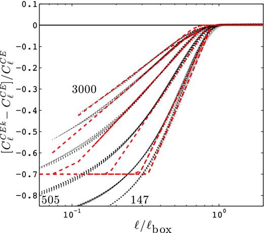
Fractional error on |$C_{\ell }^{\kappa }$| between the CE and CEk weak lensing models, for varying box sizes: Lvar = 3000, 2000, 1000, 505, 256 and 147 h−1 Mpc (we have labelled only a few of these in the figure for clarity). We stack in this figure the measurements for zs = 0.582, 0.701, 0.829, 0.968, 1.118, 1.283, 1.464, 1.664, 1.886, 2.134, 2.412, 2.727 and 3.084, and plot each of them versus ℓ/ℓbox(z) (see main text for a definition of ℓbox). All these measurements are shown with the thin dotted black lines, which superimpose remarkably well. The Lbox = 505 h−1 Mpc lines include the same calculations, carried this time with the HF2 and HF2k models. These are not distinguishable from the CE/CEk calculations, which demonstrate that the results from this figure are model independent. The thick dashed lines (red in the online version) represent the truncated power-law fits defined in equation (8).
Signal loss in |$\boldsymbol {\theta }$|-space
A similar analysis can be performed in real space for the ξ± estimator, this time as a function of θ/θbox(zs). The top panels of Fig. 4 show the amplitude loss in ξ± for the CEk models and three different zs. All measurements are normalized to CE. The (HF1k/HF1) and (HF2k/HF2) ratios produce the exact same results hence are not shown.
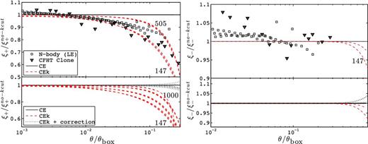
Top left: ratio between the measurements of ξ+ in the CE and CEk models. As for Fig. 2, we overplot the measurements from different sources planes and Lvar. The x-axis is the ratio between the measurement angle θ and θbox(z) (i.e. the angle subtended by the simulation box at the source redshift, see main text). The (red dashed) lines labelled 147 and 505 are actually stacked results from zs = 0.582, 0.968 and 3.084, which align very well. Also shown are stacked measurements from the LE suite (with zs = 0.582, 0.968 and 3.084, Lbox = 505 h−1 Mpc) and from the CFHTLenS CLONE (with zs = 0.5 and 1.0, Lbox = 147 h−1 Mpc). Bottom left: same models as the top panel, but with the addition of Lvar = 256 and 1000 h−1 Mpc. We also present the ‘corrected’ measurements, seen in the top right-hand region of the panel, which use equation (8) to undo the effect of the low-k cuts prior to the integration in equation (5). Right: same as left-hand panels, but for ξ−. Note the different y-scaling.
As expected, the shear correlation function falls faster as the separation angle probes physical lengths that approach the box size at the source redshift. The exact suppression factor is a strong function of Lbox. The different slopes at low ℓ shown in Fig. 2 translate into different amounts of signal loss at large θ, and can be characterized with the parameter a(Lbox). With Lbox = 505 h−1 Mpc, the signal ξ+(θ) drops by (1, 10, 25 and 50) per cent for θ/θbox(zs) being (1/100, 1/10, 1/5 and 1/4). At a tenth of a box, the 1 Gpc h−1 box misses about 5 per cent of signal, whereas the 147 h−1 Mpc box suffers from a 20 per cent loss. Exactly as observed in ℓ-space, the redshift dependence of the FS effect is absorbed in the ratio θ/θbox(z). The top right-hand panel of Fig. 4 shows the box size effect on ξ−. It follows a similar scaling as ξ+, however, the suppression occurs at larger separation angle.
The bottom two panels of Fig. 4 show how the signal for ξ± can be recovered using the correction proposed by equation (9). This is shown with the thin dotted lines that scatter around the horizontal, that are in fact regrouping corrections to the six box sizes considered in this paper. Our choice of 0.7 as the correction ceiling in equation (9) was chosen such that these dotted lines lie equally on both sides of the horizontal (i.e. a perfect correction). The new calibration is accurate to better than 5 per cent until roughly a third of the box size for ξ+ and two-thirds of the box size for ξ−.
FS correction for covariance matrices
The FS effect seen in the two-point correlation functions will unavoidably impact the four-point function as well. Since weak lensing covariance matrix are typically estimated from N-body mocks, it is critical to understand and incorporate this in the data analyses. Since the scales that are affected by the finite box are large and mostly linear, they can be described with analytical Gaussian statistics. We detail here the FS correction to the covariance about the three weak lensing observables presented in the preceding sections.
Compute the loss of power in the Cℓ measurement due to the finite simulation box size, from equation (6) or from equations (8) and (9).
Correct for the effect in the covariance measurement:
In the noise-free case, this simplifies to |${\rm FS}^{\kappa } = (1 + C_{\ell }^{\rm lost})^2 \delta _{\ell \ell ^{\prime }}$|.
We include the effect of supermodes by constructing a Gaussian shear covariance matrix from quantities with k-cuts. For 15 different source redshifts, Fig. 5 shows the relative difference between the ξ+ error bars calculated with and without the large scale k cuts, i.e. |$\Delta \sigma ^{\xi +}_G / \sigma ^{\xi +}_{\rm G\hbox{-}nokcuts}$|, where |$\sigma _{{\rm G}}^{\xi +} = \sqrt{(}\mbox{Cov}_{{\rm G}}^{\xi +}(\theta =\theta ^{\prime }))$|. The diagonal error bars were calculated following Schneider et al. (2002). We observe that the redshift dependence of the FS effect is again absorbed in the ratio θ/θbox; the scatter between the different redshifts is very small. Let us mention that the ratio |$\sigma ^{\xi +}_{\rm G} / \sigma ^{\xi +}_{{\rm G},{\rm no}\,k\hbox{-}{\rm cuts}}$| does not converge to unity at small scales because the errors depend on the integral over ξ+. The complete effect of the finite box size is therefore to produce a drop in signal at large angles, plus an overall suppression of about 2 per cent at all angles (not shown in this figure). In Fig. 5, |$\Delta \sigma ^{\xi +}_{\rm G} / \sigma ^{\xi +}_{{\rm G},{\rm no}\,k\hbox{-}{\rm cuts}}$| is manually set to zero at small θ/θbox in order to isolate the dominating large angle drop. As expected from Gaussian statistics, we note that the FS effect is the same for both the signal (ξ+) and its error bar (σξ +): for Lbox = 505 h−1 Mpc, both drop by 10 per cent at θ/θbox = 0.1. In this figure, the thin dashed lines scattered around the horizontal show the recalibration of the HF2k model with the correction factor |$f^{{\rm corr}}_{\ell }$|. We observe that the error bars agree with the HF2 to better than a per cent at all redshifts, showing the performance of the simple parametrization proposed in equation (8).
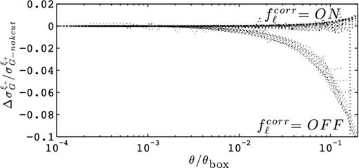
Fractional difference between the error estimates on ξ+ in the HF2 and HF2k models. We plot these results against θ/θbox(z), and stack measurements for 15 different values of the zs listed in Table 2. These all superimpose as the group of lines labelled ‘|$f_{\ell }^{{\rm corr}} = {\rm OFF}$|’. We show the effect of the correction based on equation (8) with the lines labelled ‘|$f_{\ell }^{{\rm corr}} = {\rm ON}$|’. All the curves have been normalized such that they asymptote to zero at small angles. We checked that choosing HF1/HF1k or CE/CEk produces identical results.
The real space recalibration for the FS effect follows a strategy similar to the multipole space case. With the Schneider et al. (2002) estimate
compute the predictions for ξ± from equation (5), with and without the cut-off in the lower bound of the k-integration;
compute the Gaussian predictions for Covξ ± from equations (32)–(34) of Schneider et al. (2002), both with and without the low-k cut in the ξ± predictions. Include shape noise and shot noise.
Or, with the Joachimi et al. (2008) estimate
compute the predictions for Cℓ from equation (2), with and without the cut-off in the lower bound of the k-integration; note that the k cut estimate can also be approximated from equation (9), combined with the predictions for |$C_{\ell }^{\kappa }$| without the k cut;
compute the Gaussian covariance in multipole space (|$\mbox{Cov}^{\kappa }_{\rm G}$|) from equation (12), both with and without the low-k cut; include shape noise and shot noise;
convert into |$\mbox{Cov}^{\xi \pm }_{{\rm G,no}\, k\hbox{-}{\rm cut}}$| and |$\mbox{Cov}^{\xi \pm }_{{\rm G},k\hbox{-}{\rm cut}}$| with equation (14).
VALIDATION AGAINST SIMULATIONS
The analytic correction of the FS effect, proposed in Section 3.3, needs to be verified numerical calculation. We perform this verification with two suites of N-body simulations: the CFHTLenS CLONE, thoroughly described in Harnois-Déraps, Vafaei & Van Waerbeke (2012), and a new suite, the SLICS, which is, in many ways, an upgraded version of the former. This section first details the numerical recipe of the SLICS and establishes its accuracy and limitations. The reader interested in the verification of the FS effect can skip ahead to Section 4.6.
|$\boldsymbol {N}$|-body simulations
We construct convergence and shear maps from a large ensemble of 500 N-body simulations – the SLICS-LE – that are based on the 9-year Wilkinson Microwave Anisotropy Probe (WMAP9)+baryon acoustic oscillations (BAO)+supernova (SN) cosmology, namely: Ωm = 0.2905, |$\Omega _\Lambda = 0.7095$|, Ωb = 0.0473, h = 0.6898, σ8 = 0.826 and ns = 0.969. These follows the non-linear evolution of 15363 particles inside a 30723 grid cube with Lbox = 505 h−1 Mpc, from zi = 120 down to z = 0. The initial conditions are obtained from the Zel'dovich displacement of cell-centred particles, based on a transfer function obtained with the camb online tool (Lewis, Challinor & Lasenby 2000). The N-body calculations are performed with cubep3m (Harnois-Déraps et al. 2013), a fast and highly scalable public N-body code that solves Poisson equation on a two-level mesh, and reaches subgrid resolution from particle to particle interactions inside the finest mesh. This code has been optimized for speed and minimal memory footprint, and is therefore well suited for such a task. Each simulation was performed in about 30 h on 64 nodes at the SciNet GPC cluster (Loken et al. 2010), a system of IBM iDataPlex DX360M2 machines equipped with two Intel Xeon E5540 quad cores, running at 2.53 GHz with 2 GB of RAM per core.
At selected redshifts and along each of the three Cartesian axes, the particles are assigned on a 12 2882 cells grid following a ‘cloud in cell’ (CIC) interpolation scheme (Hockney & Eastwood 1981). These ‘mass planes’ are stored to discs and serve in the construction of ‘lens planes’ in the ray-tracing algorithm (see Section 4.3). Particles themselves are temporarily dumped to disc at z = 0.640 and 0.042 for dark matter power spectrum measurements, after which the memory is released.10
As described in the cubep3m reference paper, one of the limitation from the default configuration of this code is that the force calculation at the grid scale suffers from important scatter, which effectively smoothes out some of the structure at scales up to 15 fine mesh cells. To quantify this effect and understand the resolution range on the SLICS-LE suite, we ran five simulations in a high precision mode, in which the scatter in the force is minimized by extending the exact particle–particle force up to two layers of fine mesh around each particles. These ‘high-resolution’ simulations, the SLICS-HR suite, resolve scales about four times smaller than the finer mesh.
|$\boldsymbol {P(k)}$| – simulations versus models
We could have opted for a more optimal deconvolution algorithm such as the iterative procedure proposed by Jing (2005), however, we are mainly interested in weak lensing statistics, hence this is not necessary. In the end, we estimate the isotropic power spectrum by taking the average over the solid angle: |$P(k) = \langle P({\boldsymbol k}) \rangle _{\Omega }$|. Given the number of particles and volume probed, the contribution from shot noise is negligible over the scales that matter to us, hence we do not attempt to subtract it.
Fig. 6 compares the power spectrum measured in the SLICS-LE and -HR suites at z = 0.640 and 0.042 against the three prediction models. For k < 2.0 h Mpc−1, the SLICS-LE and -HR simulations suites match the CE predictions to within 2 per cent, whereas it deviates from the other two halofit models by up to 6 per cent. The HR simulations present significant scatter at the largest scales, as expected when dealing with only a handful of realizations. For the LE sample, the mean from the largest scales (low k) is biased low by about 2 per cent, as expected from the incomplete capture of the linear regime in a finite box environment smaller than 1 Gpc (Takahashi et al. 2008). This is fully consistent with the results of Heitmann et al. (2010).
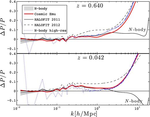
Fractional error between various power spectrum measurements and the HF1 model, at z = 0.640 (top panel) and z = 0.042 (bottom panel). The solid lines surrounded by shaded regions (labelled ‘N-body’ at high k values) represent the mean and 1σ error about the mean (i.e. |$\sigma /\sqrt{N}$|) power from the SLICS-LE simulation suite. The blue dotted lines with large scatter represent measurements from the SLICS-HR suite. Also shown are results from the HF2 and CE predictions. The HR and CE measurements exhibit the highest level of agreement.
Beyond k = 2.0 h Mpc−1, the LE simulations suite lacks power compared to CE and HF2 due to mass resolution loss, as contrasted by the HR suite that closely follows the CE model up to k = 10.0 h Mpc−1.
From these results, we reach the following conclusions.
Scales with k > 2.0 h Mpc−1 in the LE suite are affected by the resolution limits of the N-body code.
HF2 overpredicts the HR power by more than 5 per cent in the range 0.5 < k < 1.5 h Mpc−1 at z = 0.64, and in the range 0.5 < k < 4 h Mpc−1 at z = 0.042.
The CE model provides the best fit to our HR simulations up to its limit at k = 10 h Mpc−1.
Box effects are affecting our P(k) measurement by no more than 2–3 per cent, at the largest scale only.
Keeping these results in mind, let us now examine how they propagate in the light cone extracted from these simulations.
Light cone construction
Weak lensing simulations are generally constructed by integrating over null geodesics in the past light cone, using the full volume (Couchman, Barber & Thomas 1999) or a set of discrete lens planes (Martel, Premadi & Matzner 2002). The integration can either be computed along photons trajectories (Vale & White 2003) or carried on straight lines under Born's approximation. Differences between these techniques are small and occur mainly at the smallest scales, hence have no consequence on our results (Cooray & Hu 2002; Hirata & Seljak 2003). For simplicity, we work with multiple lens planes, using the Born approximation and assuming flat sky.
The choice of zmax = 3.0 – the farthest lens plane – is chosen such as to exceed the maximum source redshift of current and future weak lensing surveys. The opening angle of the light cone is set to 60 deg2, which spans 10 per cent of the simulation box at z = 0.13, 50 per cent at z = 0.75, and subtends the full Lbox at z = 2.0. We extend the light cone up to z = 3 with periodic replica. Therefore, the mass planes at z > 2 are strongly affected by the missing large-scale super k-modes, but for broad source redshift distributions, the effect on the weak lensing signal is small. In fact, the correction of the FS effect described in this paper fully accounts for this (see Section 3.1).
With the increasing importance of three-dimensional and tomographic weak lensing analyses, it has become clear that a fine redshift sampling is essential in order to capture accurately the growth of structures. With the adopted cosmology and Lbox, stacking nine simulations cubes back-to-back continuously fills the space up to z = 3, which leaves very little prospect to calibrate tomographic analyses on these simulations. We double the redshift sampling by projecting only half the simulation box, i.e. volumes that are 257.5 Mpc h−1 thick, in the construction of each of the 18 lens planes. For example, the first lens is produced by collapsing a volume whose front end is at the observer and far end at χ = Lbox/2 = 257.5 Mpc h−1. This volume is assigned to its central comoving position, i.e. at 126.25 Mpc h−1, which corresponds to z = 0.042. The second lens is collapsed at the centre of the adjacent half box, i.e. at 378.75 Mpc h−1, corresponding to z = 0.130, and so on. Generally, lens planes are generated at χlens = [(2n − 1)/4]Lbox, n = 1, 2, …
With this set-up, what we call the set of ‘natural’ source planes are those located at the rear faces of each collapsed volumes, i.e. at χs = χlens = [n/2]Lbox, n = 1, 2, … These source planes are special as they can be used in equation (19) without any interpolation in redshift. Otherwise, a measurement from a general source plane will receive contributions from a fraction of a lens, which we calculate from an interpolation between the enclosing natural source planes. The 18 lens and natural source planes are summarized in Table 2.
Redshifts of the lens planes and natural source planes that enter equation (19). These are obtained by stacking half boxes, each 257.5 h−1 Mpc thick, from the observer to zmax ∼ 3.0, given the fiducial cosmology.
| zlens | 0.042 | 0.130 | 0.221 | 0.317 | 0.418 | 0.525 | 0.640 | 0.764 | 0.897 | 1.041 | 1.199 | 1.373 | 1.562 | 1.772 | 2.007 | 2.269 | 2.565 | 2.899 |
| zs | 0.086 | 0.175 | 0.268 | 0.366 | 0.471 | 0.582 | 0.701 | 0.829 | 0.968 | 1.118 | 1.283 | 1.464 | 1.664 | 1.886 | 2.134 | 2.412 | 2.727 | 3.084 |
At the lowest redshifts, only a tiny fraction of the mass plane is used in the ray-tracing algorithm. It is tempting to recycle some of these volumes for more than one light cone, but this comes at the cost of inducing an extra level of correlation in the covariance matrix. Since this is exactly what we want to measure, we avoid this situation in the LE suite and work exclusively with independent realizations. The situation is different for the HR suite, which is not directly used for covariance matrix calculations, but rather for checking the convergence of the small scales. We therefore run only one of these costly simulation until the last lens redshift of z = 0.042, and stop the four companions at z = 0.221. For the construction of the HR light cones, we thus use five independent simulations for all lens planes with z ≥ 0.221; each is then completed with a distinct, unique, region of the z = 0.130 and 0.042 mass planes extracted from a single simulation.
|$\boldsymbol {C^{\kappa }_{\ell }}$| – simulations versus models
We compute the weak lensing power spectrum |$C_{\ell }^{\kappa }$| from each simulated convergence map with two-dimensional fast Fourier transforms,11 assuming a sky flat, and average over annuli that are linearly spaced in ℓ. This approach to the measurement suffers from some systematic effects which are worth mentioning. First, we do not take into account the non-periodic nature of the light cone, which introduces non-isotropic features in the Fourier transformed map. However, this effect is small to start with, and is further suppressed to a sub-per cent level effect during the angle averaging. Secondly, the strong interpolation inherent to the pixelization of the lower redshift planes introduces an artificial smoothing effect in addition to the intrinsic softening length of the N-body code. Although these planes are strongly down-weighted with deep lensing surveys, they systematically reduce the signal compared to a full particle light cone. Finally, even though correlations between different lenses are reduced by random rotations and origin shifting, the residual correlations translate into cross-terms in the calculation of |$C_{\ell }^{\kappa }$|, which can be of a few per cent.
Fig. 7 shows the weak lensing power spectrum for the six models of Table 1 and the ‘natural’ sources plane at redshift zs = 0.582. Other redshifts are qualitatively similar. Results are presented in terms of fractional error with respect to the HF1 model. As first pointed out in Takahashi et al. (2012), the halofit2012 calculations depart by more than 10 per cent with respect to halofit2011 for ℓ > 1000. Because weak lensing measurements project many scales on to each angle, the two models match only at the lowest multipoles. The CE lies roughly halfway in between HF1 and HF2, and features a sharp cut-off at ℓ ∼ 3000 that is caused by the exclusion of modes with k > 10.0 h Mpc−1. When the same high-k cut is applied on the halofit models (HF1k and HF2k), we see a power loss for ℓ > 1000. Consequently, one can deduce that the CE model misses about 5 per cent of power at ℓ = 3000. The SLICS-LE suite and HF1 are consistent within 5 per cent for ℓ < 6000, and are systematically lower than HF2 at all scales. As expected from the P(k) comparison described in Section 4.2, this is due to the limited mass resolution of both HF1 and SLICS-LE. Again, the CE model provides the best match to SLICS-LE over the scales that are resolved: the agreement is within 5 per cent for ℓ < 2000.
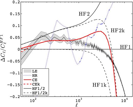
Fractional error between various weak lensing power spectrum measurements and the HF1 predictions, at zs = 0.582. We show results from the two simulations suites (LE and HR) plus all models of Table 1. The cut at k = 0.0124 h Mpc−1 impacts scales with ℓ < 60 for the source redshift considered here, hence is not visible in this figure. For the different values of Lvar considered with the CEk model, only the cut at k = 2π/147 h Mpc− 1 is visible, shown with the thick (red) dashed line. The small-scale (high k) cut at k = 10.0 h Mpc−1, common to the HF1k, HF2k, CE and CEk models, impacts all measurements at ℓ > 1000. Results from other redshifts are qualitatively similar.
With Lbox = 505 h−1 Mpc and the multipoles considered, the volume effects are negligible. We expect the effect of finite box size to be enhanced at higher redshifts, lower ℓ and for smaller simulation boxes. To explore this, we vary Lbox in the CEk predictions. Fig. 7 shows that for this source redshift distribution, the power spectrum is only affected at the lowest multipole (ℓ = 45) for Lbox ≤ 147 h−1 Mpc (see the red dashed line). In general, the signal at low ℓ is loss only when probing the missing supermodes, which occurs at z > 2 in our simulations.
|$\boldsymbol {\xi _{\pm }(\theta )}$| – simulations versus models
The shear correlation function ξ± from the SLICS simulations are measured from 500 000 randomly sampled points on the shear maps. The LE measurements of ξ+, shown in the left-hand panel of Fig. 1, agree within 5 per cent with HF1 and CE for 0.2 < θ < 20 arcmin. Finite mass resolution and finite box effects explain the loss of power outside this range of scale. HF2 is significantly higher than the simulations and the other models for all θ, consistent with the P(k) and |$C^{\kappa }_{\ell }$| comparison discussed in previous sections. The high-resolution suite exhibits a large scatter for θ > 20 arcmin that is caused by the sampling variance, but it is otherwise in agreement with the LE suite, CE and HF1 at intermediate angles. At sub-arcmin scales, HR is systematically below HF2 by 5–10 per cent.
The power loss at large separation angle seen in the simulations is reasonably well modelled by a low-k cut in the predictions (HF1k, HF2k and CEk). The fact that the measurement fall between the 257 and the 505 h−1 Mpc box predictions at large angles – rather than exactly on top of the 505 line – suggests that there are residual systematics either in our modelling or in the measurement. It is difficult to pin down exactly what causes this small discrepancy, but it is no more than 5 per cent over all angles. There is no evidence of finite box effect in ξ− for the LE suite at these angles, as expected from the theoretical calculations. For θ < 10 arcmin, the ξ− signal is strongly affected by the finite resolution of the simulations, as contrasted with the HR simulations.
Emerging structure in finite box effects: verification
We have proposed a semi-analytical correction scheme of the FS effect in Section 3.3, based on Gaussian statistics and non-linear theoretical predictions. Among the main result, we suggest that the dependence on source redshift, angle (or multipole) and the box size can be simplified with a suitable change of variable (θbox and ℓbox), which can then be modelled and corrected for. We now verify these assumptions against two weak lensing simulations suites.
While the SLICS are constructed with Lbox = 505 h−1 Mpc in a WMAP9 cosmology, the N-body simulations behind the CFHTLenS mock catalogue (Harnois-Déraps et al. 2012; Heymans et al. 2012) were based on the WMAP5 cosmology with volumes as small as 147 Mpc h−1. It was not known at that time that the box size effects had the strong impact shown on the left-hand panel of Fig. 1, although departures from predictions were indeed observed. In the construction of the CFHTLenS cosmic shear covariance matrices, some of the large-scale elements of the matrix were replaced by the Gaussian predictions to compensate for the FS effect (this was referred to as ‘grafting’ in Kilbinger et al. 2013). We come back to this topic in Section 6.
With these two simulation suites, we now investigate the FS effect on the real space cosmic shear statistics ξ+. As shown in Fig. 4, the high level of organization is also observed in both simulations suites. Three different source redshifts are shown for the SLICS (open squares), which stack on top of one another remarkably well. We also overplot the z = 0.5 and 1.0 measurements from the CFHTLenS CLONE (open triangles), after adjusting for the difference in cosmology when normalizing with respect to HF1. All simulation measurements follow their respective CEk predictions (dashed red lines labelled ‘505’ and ‘147’ for SLICS and CFHTLenS, respectively), even though the cosmology and zs change significantly. This comparison supports our claim that the proposed modelling of the FS effect can be generalized to different cosmological models, simulation codes and ray-tracing geometries.
SMALL-SCALE RECALIBRATION OF Cov|$\boldsymbol {^{\xi \pm }(\theta ,\theta ^{\prime })}$|
In the first part of this paper, we have quantified how the supermodes affect the two-point functions in real and Fourier space, and proposed a simple parametrization to correct for the FS effect on |$\lbrace C^{\kappa }_{\ell }$|, ξ±(θ)} and their covariance matrices. We validated the method against a new suite of numerical weak lensing simulations, the SLICS, which were shown to accurately model the ξ+ and ξ− signals down to 1 and 10 arcmin, respectively. In this section, we focus on the small scales of the shear correlation function covariance matrices Covξ ±(θ, θ′). We construct a prescription to recalibrate the Gaussian estimators including the FS effect, a technique that can be generalized to any simulation suite. Issues related to survey masking, beat coupling and halo sampling variance are ignored for the moment and will be discussed in Section 6.
Small angle calibration of |$\boldsymbol {\mbox{Cov}^{\xi _+}(\theta , \theta ^{\prime })}$|
Their work was based on a cosmology with a high σ8 compared to recently measured values: they used Ωm = 0.3, ΩΛ = 0.7, σ8 = 1.0, h = 0.7, and for this only, a recalibration of the fit is valuable.
All the non-Gaussian errors were chosen to be parametrized with a common power law, i.e. |${\cal F} _{S2007} \propto (\theta \theta ^{\prime })^{-\beta (z)}$|, which is a strong oversimplification. This particular choice of parametrization was motivated by the shape of |${\cal F}_{S2007}$| on the diagonal terms, which traditionally weights maximally in the forecasts based on Fisher calculations. Unfortunately, there is no quantification regarding the performance and accuracy of the fit for the off-diagonal components, even though it is natural to expect a smooth shape from the high level of correlation. What we observe in the off-diagonal elements from the SLICS is incompatible with this fit, which is why a different parametrization is necessary.
The construction of their light cones is based on the tiling technique of White & Hu (2000), which involves stitching simulation boxes of decreasing size as we approach the observer. They ran two simulations with Lbox = 800 h−1 Mpc, three with Lbox = 600 h−1 Mpc, four with Lbox = 400 h−1 Mpc and seven with Lbox = 200 h−1 Mpc. Random rotations, box ordering and origin shifting were used on 16 independent simulations to generate 64 light cones. They acknowledged the limitations of their results coming from the fact that their light cones were not independent, but the set-up adopted in this paper with the SLICS-LE simulations is a net improvement: each simulation contributes to a single light cone, as opposed to four.
The importance of finite simulation box sizes was not fully understood, and therefore Semboloni et al. (2007) did not include the k cut in the denominator of equation (21). Consequently, they found that the function |${\cal F}_{S2007}$| was crossing unity at large angles, i.e. that non-Gaussian error measured from simulations dropped significantly below the Gaussian predictions. This feature was indeed attributed to the effect of measurements on finite support, but it now becomes clear that this can be modelled accurately.
Many improvements to this fitting formula were provided in a second recalibration by Sato et al. (2011, |${\cal F} _{S2011}$| hereafter), which recognized the importance of the supersample modes in the reconnection between Gaussian and non-Gaussian measurements. Their approach was to create their Gaussian realizations numerically, i.e. explicitly embedded in their simulation box, a technique that naturally includes the large-scale (low-k) cut. Although much more accurate than the |${\cal F} _{S2007}$| estimator, the |${\cal F} _{S2011}$| is calibrated against Gaussian predictions obtained from HF1, which suffers from significant loss of power at scales of a few arcminute. This inaccuracy inevitably propagates both on the error about ξ + and on its cross-correlation coefficients. In addition, their fit function is not tested for zs < 0.6, which is unfortunate given that the peak of the galaxy distributions in many current and coming surveys lies around zs = 0.5.
Resolving these important issues justifies a new calibration of |${\cal F}_{\xi +}$|. We construct our fit function on the WMAP9 cosmology and include the 18 source redshift planes listed in Table 2. At each of these planes, we compute the Gaussian predictions with the HF2 model, and correct the FS effect in the non-Gaussian covariance matrices estimated from the simulations. The top panel of Fig. 8 shows the diagonal components of |${\cal F}_{\xi +}$| for a few of these redshifts, compared to the results from Semboloni et al. (2007) and Sato et al. (2011). Except for zs = 0.366, the |${\cal F}_{S2007}$| (dashed lines) and the simulations (squares) agree within 30 per cent down to the arcminute. Therefore, most of the gain in the current calibration comes from low-redshift planes and from the modelling of the off-diagonal elements. The agreement with |${\cal F}_{S2011}$| (dotted lines) is not as good, with significant departures at all angles and redshifts. At scales smaller than a few arcminutes, the N-body measurements depart from the power law. Since this is exactly where the progressive degradation of the mass resolution was flagged, we exclude those scales in the modelling of the recalibration. Without claiming that the power law exactly holds in these small angular scales, it is interesting to note that correcting for the mass resolution would generally improve the agreement. We leave this for a future work.
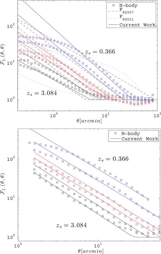
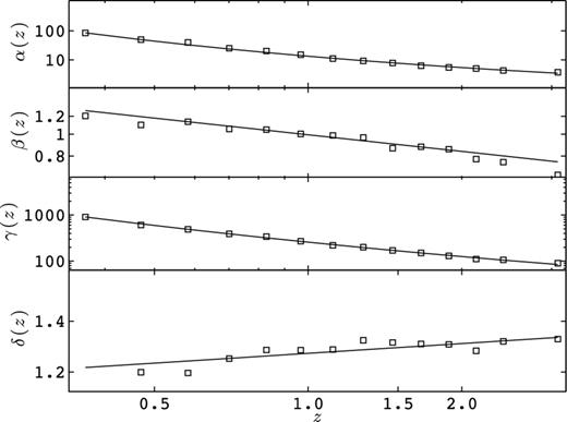
Diagonal elements of |${\cal F}_{\xi +}$| (top) and |${\cal F}_{\xi -}$| (bottom), as defined in equations (22) and (24), for zs = 0.366, 0.582, 0.968, 1.283, 1.886 and 3.084. Lower (black) symbols correspond to higher redshifts, higher (blue) symbols are for lower redshifts. The predictions from |${\cal F}_{S2007}$|, |${\cal F}_{S2011}$| and from this work are shown in dashed, dotted and solid lines, respectively.
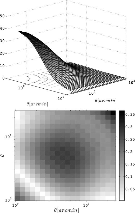
Top: full |${\cal F}_{\xi +}(\theta ,\theta ^{\prime })$| measurement at zs = 0.582. The curves shown on the x–y plane are projected lines of constant elevation. Bottom: fractional error between the measured |${\cal F}_{\xi +}(\theta ,\theta ^{\prime })$| (from the LE suite) and that constructed with the proposed fit.
Within the new parametrization provided by equation (22), fixing the diagonal elements also determines the rest of the matrix. Note that if this symmetry is preserved for a different cosmology, it is a practical and simple task to extend our result to any cosmological model, where only a fit along the diagonal of the covariance matrix needs to be carried out. We show the performance of the fit on the off-diagonal elements in Fig. 9. The agreement is better than 20 per cent for 1 < [θ, θ′] < 20 arcmin on most off-diagonal elements, and better than 30 per cent for every element down to 1 arcmin.
Small angle calibration of |$\boldsymbol {\mbox{Cov}^{\xi _-}(\theta , \theta ^{\prime })}$|
We perform an equivalent calibration for the non-Gaussian ξ− covariance matrix. As mentioned in Sato et al. (2011), the task at hand is significantly harder than for ξ+ because of the complex scale dependence of the Gaussian predictions themselves, both on and off the diagonal. These authors advocated that the error about ξ− should be calibrated directly against the N-body simulations instead. We argue in this section that a calibration matrix with good accuracy is still possible and propose the first prescription.
Fig. 11 shows the full covariance matrix about ξ− measured from N-body simulations at zs = 3.084, compared to the corresponding Gaussian predictions. Results are obtained from equation (14) without the f(A, z) correction, since this empirical correction term is calibrated specifically for |$\mbox{Cov}^{\xi _+}$|. We clearly see from the figure the reconnection between both error estimates at large angles, which occurs close to the diagonal. Lower redshifts are overall similar, except that the reconnection between Gaussian and non-Gaussian estimates occurs at larger angles.
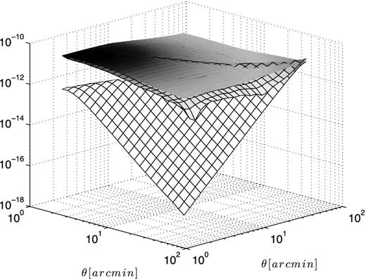
Covariance about ξ− at zs = 3.084. The top gridded surface represents the measurement from the N-body simulations, while bottom gridded surface shows the Gaussian prediction computed with the HF2 model. Note that the z-axis is in logarithmic scale. The third surface, plotted with no mesh pattern, is the result given by the parametrization of equation (25). Lower redshifts are qualitatively similar to this figure, although the connection with the Gaussian prediction occurs at larger angles and the non-Gaussian departure at small angles is amplified.
An interesting result is that no elements measured from the N-body suites appear to have negative values, in contrast with the Gaussian predictions (see Schneider et al. 2002). This is a strong hint that the anticorrelations present in the Gaussian case mostly disappear in the presence of non-linear mode coupling.
From Fig. 11, we observe that the covariance matrix for ξ− at zs = 3 also has a bell shape that peaks at |$\theta _{{\rm peak}} = \theta _{{\rm peak}}^{\prime } = 3$| arcmin with almost a circular symmetry around this peak. At lower redshifts, this peak occurs at larger angles (θpeak = 10 arcmin for zs = 0.582), but the same bell shape is observed. Generally, scales smaller than θpeak are strongly affected by limitations in the resolution of the N-body simulations, hence we expect this region of the calibration matrix to be improved with future simulations. We find that we can model the full non-Gaussian surface by rotating the diagonal of |$\mbox{Cov}^{\xi _-}$| about the peak of the bell, using only values with θ ≥ θpeak. The overall agreement between the measured and modelled Covξ − is better than 20 per cent over most of the elements at all redshifts, however, the far off-diagonal elements are generally too high by about 70 per cent. Nevertheless, this method is simple to implement, and represents a six orders of magnitude improvement over the simple Gaussian calculations.
Summary of |$\boldsymbol {\mbox{Cov}^{\xi \pm }(\theta ,\theta ^{\prime })}$| non-Gaussian calibration
Here are the prescriptions to construct the non-Gaussian covariance matrices Covξ +(θ, θ′), with a proper correction of the FS effect.
Compute the predictions for ξ+ from equation (5), without applying the low-k cut.
Compute the Gaussian error |$\mbox{Cov}^{\xi +}_{{\rm G, no}\,k\hbox{-}{\rm cut}}(\theta ,\theta ^{\prime })$| from the technique described in Schneider et al. (2002) or Joachimi et al. (2008).
Compute the diagonal components of the scaling matrix |$\cal {F_{\xi +}}$| from equations (22) and (23). The mapping between θ and Rθ is |$R_{\theta } = (\theta /0.1)^{\sqrt{2}}$|, as described in the text just before equation (22). If the sources are distributed in redshift, the best estimate uses the weighted mean of the distribution |$\bar{z}$| (see Section 6.1).
Construct the full |${\cal F}_{\xi +}$| matrix by spanning annuli in log–log space centred on θ = θ′ = 0.1 arcmin, and assigning to these elements the value found on the diagonal in step (iii).
Compute the full non-Gaussian matrix for ξ+ from the relation |$\mbox{Cov}^{\xi +}_{{\rm no}\,k\hbox{-}{\rm cuts}} = {\cal F_{\xi +}}\mbox{Cov}^{\xi +}_{{\rm G,no}\, k\hbox{-}{\rm cuts}}$|. This is meant to reproduce |$\mbox{Cov}^{\xi +, {\rm FS}}_{N\hbox{-}{\rm body}}$|, discussed in Section 3.3.
The construction of Covξ − follows similar steps.
Compute the predictions for ξ− from equation (5), without applying the low-k cut.
Compute the Gaussian variance predictions for ξ− from the method of Schneider et al. (2002) or Joachimi et al. (2008).
From equation (25), construct the diagonal components of the scaling matrix |${\cal F}_{\xi -} (\theta ) = \gamma (z)/\theta ^{\delta (z)}$|. This can be computed either at the source redshift, or, for a broad source distribution, using the weighted mean redshift, as described in Section 6.1.
Construct the diagonal of the non-Gaussian matrix Covξ − from equation (24): |$\mbox{Cov}^{\xi -}_{{\rm no}\,k\hbox{-}{\rm cuts}} = {\cal F_{\xi -}}\mbox{Cov}^{\xi -}_{{\rm G,no}\,k\hbox{-}{\rm cuts}}$|.
Find the angle where this function is maximal (e.g. θpeak = 3 arcmin at zs = 3 and 10 arcmin at zs = 0.58) and rotate the diagonal elements about this maximum to generate the off-diagonal matrix elements Covξ −(θ′ ≠ θ). For this step, only consider the contribution coming from θ ≥ θpeak.
The presence of shape noise σϵ adds a new contribution to the Gaussian component, as seen in equation (12), but the calibration matrices presented in this section are only valid in the noise-free case. It would be wrong to calculate |$\mbox{Cov}^{\xi -}_{{\rm G,no}\,k\hbox{-}{\rm cuts}}$| with shape and shot noise included, and to apply the |${\cal F_{\xi \pm }}$| matrices afterwards. Instead, the correct thing to do is
work out the noise-free case |$\mbox{Cov}^{\xi \pm }_{{\rm no}\,k\hbox{-}{\rm cuts}}$|;
subtract the noise-free Gaussian component |$\mbox{Cov}^{\xi \pm }_{{\rm G,no}\,k\hbox{-}{\rm cuts}}$|;
add new Gaussian contribution that includes the noise, using equations (12) and (14).
Recall that the Gaussian covariance of real space cosmic estimator is not diagonal, hence the inclusion of shape and shot noise described above affects all elements, even those for which θ′ ≠ θ. The cosmological dependence of |${\cal F}_{\xi \pm }$| is beyond the scope of this paper and will be investigated in a future work.
APPLICATION TO REDSHIFT SURVEYS
In this section, we integrate the core results of this paper into a realistic framework that incorporates extended distribution of sources and survey masks.
Broad redshift distributions
Whether weak lensing is measured with a narrow or broad source redshift distributions, the true distribution n(z) is never a single redshift sheet. It is therefore important to extend the previous work to a broad redshift distribution, extracted from the data and usually well described by analytic functions.
We do recover a power suppression in both Fourier and real space, which fits well in our FS formulation if the source is taken to be at the weighted mean redshift |$\bar{z}$|. The shape of the power loss stacks very well on top of the measurements at discrete zs shown in Figs 2 and 4, meaning that we can use the prescription based on the |$f^{{\rm corr}}_{\ell }$| correction term by employing |$\bar{z}$| in all the fitting function presented in this paper. We also checked that the calibration matrices |$\cal {F}_{\xi \pm }$| were consistent with the predictions at |$\bar{z}$|, both its shape and amplitude. Generally, the added complexity coming from dealing with a broad n(z) reduces the accuracy of our correction to the FS effect by no more than 5 per cent, compared to the discrete plane case.
Signal and error calibration with survey mask
Masking is unavoidable in gravitational lensing analyses because of the bright stars, satellite trails, etc., that need to be removed from the images. We describe here how to address the FS effect in the presence of a general survey mask.
Mask applied on the mock catalogues
Masking is included in mock galaxy catalogues by applying the observed survey masks to the simulated light cones and weight each mock galaxy (or pixel) by the mask value. Once this is done, the mock catalogues have both the k cuts and the mask included, and as such should be compared to a theoretical model that also accounts for these two features. The effect of masking is described as the product of the underlying density field and the mask in real space, or as a convolution of the Fourier space quantities. The convolution of the theory |$C_{\ell }^{k\hbox{-}{\rm cut}}$| with the mask's power spectrum therefore gives the desired prediction, |$C_{\ell , {\rm mask}}^{k\hbox{-}{\rm cut}}$|, and one can then use equation (5) on this quantity to compute the model for |$\xi _{\pm , {\rm mask}}^{k\hbox{-}{\rm cut}}$|. This provides a consistent baseline between the masked mock catalogues and a theoretical signal, which is essential whenever one needs to test or calibrate a weak lensing estimator on the masked mocks.
Note that in this case, the FS effect is correctly accounted for, but not corrected. Also note that the actual data are not affected by the k cut, hence should be compared to Cℓ, mask and ξ±, mask. The calculation of two theoretical models – with and without the k cut – is therefore necessary. In certain cases, it could be possible to deconvolve the mask from the mock observations, yielding an estimate of |$C_{\ell }^{k\hbox{-}{\rm cut}}$| that can then be corrected with |$f^{{\rm corr}}_{\ell }$| and compared to the model Cℓ with no mask and no k cut.
Mask applied on the two-point function
One of the advantages of the mock catalogue over real data is that the masking can be added or removed at will, allowing for a careful understanding of its impact on the measurement. As an alternative to weighting the mock galaxies, one can also conduct the two-point function analysis on the simulations without the mask first, then integrate the effect of masking on the two-point function afterwards. This becomes advantageous notably for Cℓ measurements since, as an intermediate step, one can use the tools provided in this paper to undo the FS effect from the unmasked mocks – with the |$f^{{\rm corr}}_{\ell }$| correction term – and convolve the corrected measurement with the mask subsequently. This would make the measurement from the simulations fully consistent with the data, and both could be compared to a unique prediction, i.e. Cℓ, mask (with no k cut). For the ξ± measurements, this is even simpler since the mask has no effect on the mean, only on the error. It is therefore only a matter of correcting the mocks for the FS effect, then one can directly compare the data and the simulations with the ξ± model (with no k cut).
Mask and covariance
The covariance matrix calculations in presence of a survey mask contain a higher level of complexity: in addition to the FS effect described in this paper, two complimentary finite box contributions must be included: the halo sampling variance (HSV) and the beat coupling (BC). We briefly review the origin of these two quantities, then expose our strategy to incorporate them all in a consistent manner.
The HSV term comes from the finiteness of the simulation volume which imposes a constant density at the simulation box scale (this is the same across all realizations). A larger box size, |$\widetilde{L}_{\rm box} \gg L_{\rm box},$| allows fluctuations at the scale of Lbox, thereby producing more massive haloes and larger voids that contribute significantly to the total variance at Lbox. Their absence results in a missing variance in the smaller box simulation. This quantity is labelled Covκ, HSV and can be estimated analytically following Sato et al. (2009), then added to the sampling variance measured from the simulations. Unfortunately, this estimation is not very accurate at the moment, and more work will be required in order to capture Covκ, HSV accurately.
The BC term, first identified in Rimes & Hamilton (2006) and Hamilton, Rimes & Scoccimarro (2006), comes from the interaction between the survey mask and the ‘true’ covariance. In N-body simulations this interaction vanishes, hence an error estimate based on unmasked mocks will underestimate the ‘true’ error. The correct error, Covκ, obs, can be written as a two-dimensional convolution of the ‘true’ covariance with the mask power (Takada & Jain 2009), and the BC contribution is generally represented by Covκ, BC = Covκ, obs − Covκ, true. Its contribution on P(k) at the survey box scale can be modelled analytically to better than 10 per cent accuracy (Li, Hu & Takada 2014), which can then be propagated on to Covκ, BC as in Takada & Jain (2009).
To estimate the error on real space quantities, one can then use equation (14) on each term of equation (27) to produce Covξ ±, HSV and Covξ ±, BC as in Takada & Jain (2009), but also |$\mbox{Cov}^{\xi \pm , {\rm FS}}_{N\hbox{-}{\rm body}}$|. This last term is a bit trickier: simulated light cones do not cover the full sky, while this calculation involves an integral over all ℓ. One needs to include the contributions from ℓ < ℓlight cone by grafting a Gaussian covariance matrix, as done in Kilbinger et al. (2013). Although completely equivalent, it seems simpler to compute |$\mbox{Cov}^{\xi \pm , {\rm FS}}_{N\hbox{-}{\rm body}}$| as in equation (15), i.e. by correcting the simulation measurements directly in real space.
Since the masks reduce the effective area of the survey, one must finally scale up the total error by the ratio between the unmasked area and the simulated light cones.
One ingredient that is currently missing from the error calculation is the interaction between the mask and the covariance at small scales. The masking procedure inevitably introduces an extra level of non-Gaussianity, and these are not accounted for in the current prescription. It is hard to predict the significance of this contribution, but we intend to follow the approach of Harnois-Déraps & Pen (2012) and quantify its importance in a future work.
CONCLUSION
Simulations are central to weak lensing data analyses for calibration and verification of estimators, for studies of systematics linked to secondary signals, but also to provide an accurate description of the errors about the measurement. In this paper, we investigate the impact of finite box size on weak lensing measurements performed in simulations and identify a new contribution to the uncertainty that has been overlooked in the past, which we coin the finite support (FS) effect. This contribution arises from the missing supersample modes that produce a suppression of the two-point function at large scales, which leaks into higher order statistics.
We predict the impact of the FS effect for measurements of |$C_{\ell }^{\kappa }$|, ξ+ and ξ −, and propose simple recipes to rescale the measured signal and covariance. The rescaling factors primarily depend on the simulation box size Lbox and on the ratio θ/θbox(zs) (or ℓ/ℓbox(zs)), but are independent of the choice of theoretical model – minimal variations are observed among halofit2011, halofit2012 and the CE. We verify these calculations against two series of N-body simulations: the new SLICS-LE suite with Lbox = 505 h−1 Mpc, and the CFHTLenS CLONE, which has Lbox = 147 h−1 Mpc.
The lensing power spectrum |$C_{\ell }^{\kappa }$| is negligibly affected by the FS effect as long as the physical scales that are probed are fully contained within the simulation volume. For the largest scales and highest redshift, simulated light cones often escape the volume, causing the amplitude of the power spectrum to drop. This loss can be accurately captured analytically by simple functions of Lbox and is easily corrected in the signal (see equations 8 and 9) and in the covariance (see equation 13).
Real space cosmic shear estimators like ξ±(θ), however, are more sensitive to box effects, even at scales well inside the simulation volume. This can be understood from their dependence on the integral over the power spectrum, causing any missing large-scale k-modes to affect a wide range of angles. Specifically, if the ratio θ/θbox(zs) = 0.1, ξ+(θ) and its error are suppressed by 5, 10, 20 and 25 per cent for Lbox = 1000, 500, 250 and 147 h−1 Mpc, respectively, independently of the source redshift. For θ/θbox(zs) = 0.2, the suppression exceeds 25 per cent even for Lbox = 1 Gpc. With our simple parametrization (see equation 15), we can undo this FS effect with high fidelity, both in the signal and the error: the residual differences between the corrected simulations and the continuous theory model (i.e. with no missing large-scale modes) are generally of a few per cent only at all angles, even for volumes as small as those used for the CFHTLenS CLONE.
We discuss how all known finite box effects might be incorporated in a weak lensing data analysis, in the presence of a broad distribution of source redshift and including survey masking. In the light of these results, the precision challenge exposed in Section 1.1 seems to have a solution. We advocate for an estimation strategy of the covariance based on large ensembles of simulations with sub-Gpc volume that accounts and corrects for finite box effects, as opposed to subvolume resampling a mock sky based on a single Gpc simulation. A lower bound on the volume is placed by the requirement that (1) large scales reconnect with the Gaussian statistics, and (2) baryon feedback effects must vanish at the largest scales. This suggest that Lbox should be at least a few hundreds of Mpc h−1.
In the second part of the paper, we propose a revised calibration matrix |${\cal F}_{\xi +}$| and the first |${\cal F}_{\xi -}$| partner that map Gaussian calculations on to non-Gaussian covariance estimates about ξ+ and ξ−, respectively. These two objects are essential for accurate forecasting and parameter extraction based on Markov chain Monte Carlo methods. Our fits for |${\cal F}_{\xi \pm }$| involve only five numbers that we determined with 15 redshifts checkpoints from the simulations. |${\cal F}_{\xi +}$| is confirmed to hold an element-by-element accuracy of 20–25 per cent for z < 3 and θ > 1.0 arcmin, even in the far off-diagonal regions. |${\cal F}_{\xi -}$| is also 20 per cent accurate over the diagonal and most of the (θ, θ′) plane, but some of the far off-diagonal elements show larger deviations.
Many ideas presented in this paper could easily be extended to other fields of cosmology that rely on simulations, notably cross-correlation studies of weak lensing maps with galaxy fields or other tracers of matter. The FS corrections play a key role to guarantee the accuracy of calculations based on simulated mock catalogues. So far, the modelling of the FS effect has been tested on |$C^{\kappa }_{\ell }$|, ξ± and their respective covariances, and extensions to other common cosmological observables (angular clustering functions, aperture mass, etc.) should be straightforward. It is our hope that such extensions will become available in preparation for future large surveys.
The authors would like to thank Chris Blake and Tim Eifler for their comments on the manuscript, and acknowledge significant discussions with Benjamin Joachimi and Masahiro Takada about finite box effects in general. Computations for the N-body simulations were performed on the GPC and TCS supercomputers at the SciNet HPC Consortium. SciNet is funded by: the Canada Foundation for Innovation under the auspices of Compute Canada; the Government of Ontario; Ontario Research Fund – Research Excellence and the University of Toronto. JH-D is supported by a CITA National Fellowship and NSERC, and LvW is funded by the NSERC and Canadian Institute for Advanced Research CIfAR. This work was supported in part by the National Science Foundation under Grant No. PHYS-1066293 and the hospitality of the Aspen Center for Physics.
See Section 2.3 for a definition of the ξ± quantities.
To the best of our knowledge.
It is important not to confuse Lbox (the size of the simulation volume, in units of Mpc h−1) with ℓbox (the multipole corresponding to an object of size Lbox on the sky, which is a redshift-dependent quantity).
In these two references, the notation for the weak lensing power spectrum measured in E/B-modes is PE/B(ℓ), but we label these quantities by |$C_{\ell }^{E/B}$| here for consistency with the rest of the paper, and set the B-channel to zero.
Following Sato et al. (2011), this pre-factor can be written as |$f(A,z) = {\rm max}(\alpha _z/A^{\beta _z},1.0)$|, with αz = 3.2952z−0.316369 and βz = 0.170708z−0.349913. We note that this correction factor was calibrated for a slightly different cosmology, but this has a marginal effect on our calculations in the end.
We also produced dark matter haloes at the redshifts of the mass planes from the on-the-fly spherical overdensity halo finder described in Harnois-Déraps et al. (2013). However, these haloes are not part of the current paper, hence we leave their description for future work.
Following the three-dimensional case, we minimize the impact of the grid assignment scheme with a two-dimensional version of equation (16).
