

Abstract
This work aims to optimize the overall performance of a model oscillator, as an energy harvester of Lévy-like mesoscopic fluctuations through piezoelectric conversion. As a further step in the description of a realistic harvesting device we consider a monostable Woods-Saxon oscillator, which can interpolate between square well and harmonic-like behaviors. We study the interplay between the potential shape and the noise's spectrum and statistics. The dependence of the power output on the parameters determining those features indicates the directions in which the former can be increased.
Export citation and abstract BibTeX RIS
Introduction
Noise is a paradigm of the unwanted features in engineering. For instance, the trend to lower operating voltage (and hence dynamic energy loss) in digital technology is limited by the "noise margins". In science however, the appraisal of the role of fluctuations has changed during the last century, from being just a nuisance or a deviation from an expected behavior to being the source of a plethora of amazing and potentially useful phenomena [1, 2] (remarkably known examples being stochastic resonance [3–5] and Brownian motors [6, 7]). The key to this shift in perception is its highly nontrivial interplay with nonlinearity, especially when the noise interacts "multiplicatively" (namely, by affecting parameters of a nonlinear system). This fact prevents, on the other hand, results obtained with Gaussian white noise to be taken at face value for either colored spectra at the operating frequency range [8, 9] or noise statistics not obeying the central-limit theorem [10, 11]. The present challenge of nanotechnology is forcing a similar reappraisal of noise on the side of engineering.
Among the fields where engineering could promptly take profit from noise is "energy harvesting" [12–21], a category which fits solar, aeolic, tidal and ocean-wave energy conversion (to name but a few classical sources) and also energy conversion from macroscopic vibrations, through (linear) resonance-like properties of the devices. Without detriment to those applications, modern technology prompts us to solve Achilles' heel of small devices, namely to substitute batteries: they severely constrain the devices' size and weight reduction on the one hand, and their need to be periodically recharged (and even replaced) limits their autonomy and ubiquity.
No doubt energy is a scarce input at all scales but perhaps with the exception of electric cars and domotic embedded systems, the challenge that modern life poses to energy consumption is increasingly towards the small, portable device range. Some of the significant applications include wireless sensor systems [22–24], self-powered microelectronics [25–27], autonomous battery recharging [28, 29], and many other applications (see, e.g., [30, 31]). The solution of extracting useful work out of those motions present in the ambient which we usually regard as "noise" or "fluctuations" (thermal noise, light, potential differences in living tissue) then becomes more and more convenient. In this context, it is possible to conceive devices (meteorological stations, mechanical acquisition or control devices, etc) which —mimicking what living cells do all the time, by absorbing oxygen and nutrients from their surroundings in an autonomous fashion— could operate indefinitely in their medium without frequent maintenance.
Now, linear devices are ill-suited to answer this challenge since they exhibit resonance within a very narrow frequency range. In order to increase their efficiency, research has begun to explore active and semi-active strategies [32–34]. A new and innovative approach —pioneered by Gammaitoni et al. [35–38]— calls for nonlinearity as a central ingredient. A nonlinear oscillator can pick energy up from a wider range of frequencies than its linear counterparts, thus better exploiting the available noise energy. Now, much as a linear oscillator needs tuning in order to maximize the energy harvested in a particular situation, a nonlinear one would need to adjust its parameters to optimally respond to a noise having certain spectral and statistical features.
In this letter we elaborate on recent work by Gammaitoni et al. [37], and consider a monostable nonlinear oscillator connected to a piezoelectric device and submitted to correlated noise (in our case, eventually with asymptotic power-law statistics). Whereas the amplitude of the noise and its statistical and spectral properties are to be taken as data, one can tailor the shape of the nonlinear potential in order to maximize the energy production. Here we propose a model potential which —being able (as the even-power potentials of ref. [37]) to interpolate between harmonic and hard-wall ones— is more realistic in the sense that it exhibits a finite range, which can be controlled by means of a parameter as well as the wall steepness and the potential depth. This potential provides not only the nonlinearity needed for the wide-spectrum energy-harvesting approach but also, a more realistic scheme for future technological applications and a simple way to compare with the linear case. We consider the effects of both Gaussian and non-Gaussian noise statistics on the power production as they interact with the nonlinear system.
The model
Following ref. [37] we consider a one-dimensional anharmonic oscillator governed by a monostable potential U(x), which mediates between a source of stochastic mechanical vibrations producing an instantaneous force η(t), and a piezoelectric transducer producing a voltage V (t) = Kc x(t). In turn, the transducer reacts back on the oscillator with a force Kv V (t), i.e., neither delay nor nonlinearity are assumed.
The voltage V is to be applied to an external load, modelled as a constant resistance R. But there is also some capacitance C (due partly to the external circuit but mainly to the piezoelectric transducer itself) so the response will exhibit some delay, encoded in its time constant τp = RC. Let m and γ be, respectively, the oscillator's mass and viscous friction coefficient, and σ the coupling to the stochastic source. Then x and V obey the stochastic differential equations


The stochastic force η(t) will be characterized below.
For  in eq. (2), Vrms = Kc xrms, where xrms is the r.m.s. departure of the oscillator from its equilibrium position. Since the power delivered to R is P = V2rms/R, xrms is a gauge of power production.
The Woods-Saxon potential
In ref. [37], U(x) has been modeled as an even power of x, up to order 20. We instead choose the form proposed in the mid fifties by Woods and Saxon as a mean-field potential for single-nucleon states within the shell model of nuclear structure [39]
This heuristic potential with three parameters reproduces the qualitative features of the mean force exerted on each nucleon inside the atomic nucleus (fig. 1). It takes the values −V0/(1 + e−R/a) for |x| → 0, −V0/2 for |x| = R and zero for |x| → ∞, becoming a square well of depth V0 and width 2R for a → 0. As a grows the potential walls become smoother, maintaining the value −V0/2 at |x| = R. For a large enough, U(x) resembles a harmonic potential for R ≫ a and |x| > a. Hence we too can (as in ref. [37]) monitor the deviation from the linear case by varying just one parameter (a in our case), whereas avoiding unreal infinite walls.
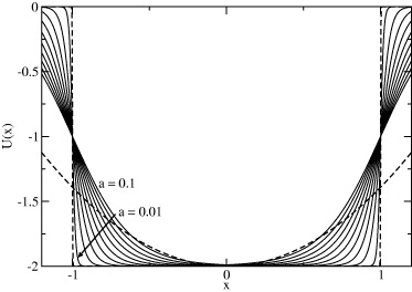
Fig. 1: Shape of the Woods-Saxon potential (WSP), eq. (3), for V0 = 2 and R = 1, and a varying from 0.01 to 0.1 in steps of 0.01. Dotted lines: square well (which the WSP approximates for a → 0) and a harmonic oscillator, which the WSP resembles at finite a, for R,|x| > a.
Download figure:
Standard imageNon-Gaussian noise
In [37], η(t) has been modeled as an Ornstein-Uhlenbeck (OU) noise with zero mean, unit variance and exponential autocorrelation with characteristic time τ. Whereas Gaussian noise sources with finite autocorrelation time offer a more realistic scenario than the white-noise approach, they still disregard two facts: that many real-life vibrations and noises are not Gaussian, and that energy appears often distributed as f−β. Since we assume that we can only control the energy-harvesting device, it is significant to study its performance under fluctuations obeying more general statistics and spectral distributions, so to know what to expect in a realistic environment. A class of colored (although not Lorentzian, but f−β [40]) non-Gaussian noises depending on one more parameter besides τ, is dynamically generated by the following system [10, 41–45]:

where ξ(t) is a white noise of zero mean and correlation 〈ξ(t)ξ(t')〉 = 2δ(t − t'), τ is the self-correlation time and

So defined, η is a colored non-Gaussian noise obeying a q-exponential distribution. Some analysis shows that for q > 3, η(t) is not normalizable; for 1 < q < 5/3 the distribution resembles a Lévy one, and for q < 1 it is a cut-off distribution. For q = 1, we recover the Gaussian distribution and η(t)q=1 is nothing but an OU noise.
We have centered our efforts in q > 1. In this case the statistics of the noise are of potential type. This genre of fat-tailed distributions have been shown to be ubiquitous in nature, and many types of vibrations exhibits this kind of statistics instead of the Gaussian type. The most important factor which differentiates them from the Gaussian noises is the non-negligible probability of large deviations from the mean value of the noise. These events may be used by the harvester to extract useful work. We have studied the dependence on the potential parameters of the system's performance for q ranging from 1 to 1.2 and several values of τ.
Results
Since our aim is to optimize the monostable potential U(x) with regard to power generation out of a colored non-Gaussian noise η(t), we set the parameters m, γ and Kv in eq. (1), Kc in eq. (2) and R in eq. (3) to unity for simplicity, and τp = 104 in eq. (2) for ease of comparison with the results of ref. [37]. We have integrated the dynamic eqs. (1), (2) and (4) by Heun's method, with the monostable potential U(x) and the "noise potential"Vq(η) defined, respectively, by eqs. (3) and (5). Key parameters in this work are q in eq. (5) and a in eq. (3).
We started the simulation from a random set of initial conditions and after a transient, computed Vrms from eq. (2). An ensemble average of 103 realizations has been performed for each set of parameters1. We have repeated the simulation for different values of σ in eq. (2) and τ in eq. (4), and studied the power generation of the system as we vary V0 and a in eq. (3), and q in eq. (5).
q = 1
As a first step, we study the performance of U(x) for OU noise. In fig. 2 we have chosen τ = 10 as in ref. [37]. In the left frame we have kept V0 = 0.5 and varied a, noticing an improvement for higher values of σ as we make the potential smoother. This effect is more noticeable in the right frame where V0 = 1, since the dependence on σ which somehow masks it is suppressed. In both cases, the improvement is achieved by favoring situations in which |x| > R.
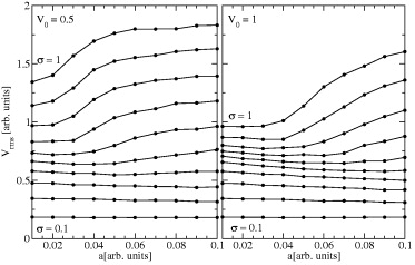
Fig. 2: Vrms as a function of a, for τ = 10 and σ varying from 0.1 to 1.0 in steps of 0.1. Left: V0 = 0.5; right: V0 = 1.0. The benefical effect of smoothing (for strong enough noise) is more pronounced for a deeper well.
Download figure:
Standard imageThe performance as a function of τ is summarized in fig. 3, for selected values of σ and a. As is best appreciated for σ large enough, the performance is optimal for small (but nonzero!) correlation times (around τ = 0.25 for σ ⩽ 0.5). This is a consequence of the relatively strong damping resulting from our choice γ = m = 1.0.
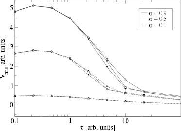
Fig. 3: Vrms as a function of τ for V0 = 1.0, σ indicated in the figure and three values of a: 0.1 (•), 0.5 (□), and 0.9 (△). For σ large enough, the performance is optimal for small correlation times (around τ = 0.25).
Download figure:
Standard imageq > 1
Now we monitor the performance of the system as q increases above 1. In fig. 4 we have done so for four values of the noise amplitude σ, and ten of the potential depth V0. We have fixed a = 0.05 so U(x) is not so steep but still away from the harmonic limit. The first noticeable feature is the almost linear increase of Vrms with q, for σ and V0 high enough. For σ = 0.8 (higher left frame), almost nothing new is learnt: Vrms is higher (even at q ≈ 1.0) the higher V0 is, indicating that the well acts simply as a selector on the basis of noise strength.
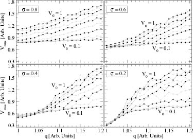
Fig. 4: Vrms as a function of q for a = 0.05, four values of σ and ten of V0 (odd values in gray, even ones in black). For low σ (lower frames), Vrms decreases with V0 for 1 ⩽ q ⩽ qX and then rises spectacularly with q and V0, until some saturation in terms of q (clearly visible in the lower right frame) occurs.
Download figure:
Standard imageThe true gain comes for weak enough noise (lower frames): whereas for Gaussian noise the system remains confined within the well (with shallower wells slightly better performing), a crossing occurs at some qX (≈1.05 for σ = 0.4 and 1.02 for σ = 0.2) and its r.m.s. displacement rapidly scales as q increases, reaching for q ≈ 1.1 the levels achieved at higher σ. The most spectacular case is σ = 0.2 (lower right frame): for a deep well V0 = 1, Vrms is 0.3 at q = 1 and 1.5 at q ≈ 1.1.
A similar behavior is found when one fixes V0 = 1.0 and varies a (fig. 5). The main difference is that no crossing occurs for low σ, so that a steep potential (a small) always yields the best performance.
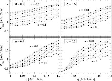
Fig. 5: Vrms as a function of q, for V0 = 1.0 and four values of σ; a increaseses downwards, in steps of 0.01 (odd values in gray, even ones in black).
Download figure:
Standard imageConclusions
Our focus in this work has been the performance as piezoelectric energy harvester of a weakly damped monostable 1D oscillator, submitted to an asymptotically power-law distributed colored noise. In a regime where Vrms∝xrms, it will be dominated by large excursions of the oscillator. These are allowed by a finite-range potential like the Woods-Saxon one we have proposed, whereas they are suppressed by the even-power potentials considered in ref. [37].
Because it depends on only two parameters with clear interpretation and it is easy to generate dynamically by means of eq. (4), we have chosen as external noise the process defined by eq. (5). Following ref. [37] and for the benefit of this study, we have regarded the noise amplitude σ as a parameter under our control. Whereas this is not impossible, to do so (e.g., through double electrical conversion and an OpAmp, or directly through a lever) would imply energy consumption. A more realistic interpretation would be to assign the variance 〈ξ(t)ξ(t')〉 = 2σ2δ(t − t') to the driving white noise ξ(t) in eq. (4). In such a situation, what fig. 4 tells us is that a moderately round and deep enough square well acts as a great selector of large excursions and is thus able to take the most out of a very weak Lévy-like fluctuation.
Acknowledgments
Financial support for this work has been granted by MINECO (Spain) through Project FIS2010-18023 (HSW), from MECD (Spain) through Sabbatical SAB2011-0079 (RRD), and from UNMdP (Argentina) through Project EXA544/11 (RRD).
Footnotes
- 1
Despite the fact that as q grows, the noise becomes more and more "fat-tailed", most curves in figs. 2–5 appear rather smooth. In order not to obscure the information in the figures, we have chosen not to draw the error bars arising from ensemble averaging. We believe the uncertainty expected on the simulated data to be best read off from the curves' roughness.