


Abstract
We present a new technique to study preferential concentration of inertial particles in (active) grid generated turbulence. This method, based on the use of a Taylor hypothesis combined to high-speed imaging, allows to reconstruct unprecedentedly long fields of particles and therefore to analyse new large-scale features, not easily resolvable with standard high-speed imaging methods. We first show that the new approach robustly reproduces results on particles clustering previously reported from standard methods. We then extend the analysis to show the first evidence of superclustering (existence of clusters of clusters) of inertial particles in turbulence and present the first characterization of superclusters.
Export citation and abstract BibTeX RIS
Introduction
Turbulent flows laden with particles are frequent in natural and industrial situations such as atmospheric dispersion of pollutants, sedimentation in rivers, rain formation, plankton dynamics in seas, optimization of chemical reactors and various industrial processes including combustion of liquid fuel, among others. In these examples, particles consist of dust/sand in air or water, liquid droplets or solid particles (such as coal, catalyst, ...) in gas and are then denser than the carrying fluid. Thus, their dynamics is not strictly following that of the carrier fluid but is instead lagging behind it. This is a specific case of inertial particles immersed in turbulent flows that also refer to situations where particles are less dense than the fluid or when the particle size is greater than the smallest turbulent scale.
A striking feature of turbulent flows laden with inertial particles is the so-called preferential concentration phenomenon which leads to strong inhomogeneities in the concentration field at any scale. This has now been widely observed in many experimental and numerical configurations including homogeneous isotropic turbulence [1–3]. Particles interacting with a turbulent flow are then commonly characterized by their Stokes number St, that is, the ratio between the particle viscous relaxation time  and a typical time scale
  of the flow (in the context of turbulent flows
  is traditionally chosen to be the Kolmogorov dissipation time
  ).
).
We present here experimental evidence that not only inertial particles in turbulence tend to form clusters, but that the clusters are themselves segregated in larger structures, namely superclusters (i.e. clusters of clusters). To this aim, we propose a new method to reconstruct large-scale concentration fields of particles from regular high-speed imaging acquisitions, as for instance exploited in [4,5]. We use the experimental data analyzed in those previous wind tunnel measurements to reconstruct a concentration field of particles over spatial scales exceeding the actual measurement volume defined by the field of view of the camera. The idea is based on an extension of the classical frozen field Taylor hypothesis (commonly used to reconstruct spatial profiles of velocity fields from hot-wire time-series in wind tunnels for instance) applied to high-speed imaging.
From these large-scale fields, we can analyse the large-scale structuration of clusters of particles. Using Voronoï analysis [6,7], we show the evidence of superclustering and present the first geometrical characterization of superclusters.
Experimental setup
Experiments are conducted in a wind tunnel with a measurement section 4m long and a square cross-section of  (fig. 1). More details of this experimental setup can been found in [4]. Turbulence is generated with an active grid. Five different mean velocities have been explored, ranging from 3.4 m/s up to 7.6 m/s, corresponding to a range of Reynolds number (based on the Taylor microscale
  , where u is the fluctuating velocity,
  the turbulent energy dissipation and ν the kinematic viscosity of the flow)
 ![$Re_\lambda \in [230; 400]$](https://content.cld.iop.org/journals/0295-5075/112/5/54004/revision1/epl17562ieqn7.gif) . Table 1 summarises the main turbulence parameters of the flow generated at the measurement volume location (3 m downstream the active grid) for the 5 mean wind velocities investigated. These parameters were obtained with hot-wire anemometry. As inertial particles we use small water droplets generated by 36 high-pressure atomizers (distributed on a
. Table 1 summarises the main turbulence parameters of the flow generated at the measurement volume location (3 m downstream the active grid) for the 5 mean wind velocities investigated. These parameters were obtained with hot-wire anemometry. As inertial particles we use small water droplets generated by 36 high-pressure atomizers (distributed on a  mesh with identical spacing to the grid) located in a transverse plane 15 cm downstream the grid. The droplets size distribution (measured with a Spraytec diffractometer from Malvern Instruments Ltd) is peaked around a most probable droplet diameter of the order of
  , but is relatively polydisperse (the standard deviation of particles diameter is
  ). This distribution is not significantly affected by changes in
  . The most probable Stokes number St is then estimated as
  , with η the dissipation scale of the carrier turbulence and
  the water to air density ratio.
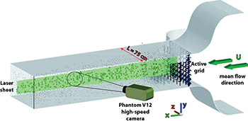
Fig. 1: (Color online) Sketch of the experimental setup.
Download figure:
Standard imageTable 1:.
Experimental parameters: Reynolds number based on the Taylor microscale  , mean wind velocity (U), energy injection scale (L), dissipation scale (η), energy dissipation rate per unit mass () and Stokes number (St).
 |
U (m/s) | L (cm) | η (μm) | (m2s−3) |
St |
|---|---|---|---|---|---|
| 234 | 3.4 | 13.0 | 280 | .69 | 2.1 |
| 264 | 4.0 | 13.2 | 240 | 1.2 | 3.3 |
| 331 | 5.7 | 13.8 | 178 | 3.4 | 5.8 |
| 357 | 6.4 | 14.0 | 160 | 4.7 | 6.6 |
| 400 | 7.6 | 14.3 | 140 | 7.7 | 9.9 |
Acquisitions were performed using a Phantom V12 high-speed camera operated at a sampling frequency Fs of 10 kHz and acquiring 12 bits images at a resolution of  corresponding to a 125 mm (along x) ×55 mm (along y), though homogeneous illumination conditions (tested a posteriori during the post-processing) were actually limited to a smaller visualization window of 70 mm in the streamwise x-direction and 50 mm in the transverse y-direction. Therefore, the explored domain covers a significant fraction of the integral scale of the carrier flow in each direction. The camera is mounted with a 90 mm macro lens; the view angle with respect to the laser sheet is of the order of 60° (to increase particles image brigthness); a Scheimpflug mount is used to compensate the loss of depth of field. At the given spatial resolution and repetition rate, the onboard memory of our camera (8 Gb) allows to record about 104 images (hence slightly more than one second of recording), which corresponds already to a few integral time scales of the carrier turbulence. For each experimental configuration we acquire at least 15 such recordings, thus a set of more than 1.5 · 105 images are obtained for each experiment.
Reconstruction of linear fields
The usual analysis of preferential concentration of particles exploits individual images as shown in fig. 2(a) to identify particle centers and then perform any sort of diagnosis (such as box counting methods, estimates of pair correlation functions, Voronoï diagrams, etc.) [7]. Such an approach has the drawback that the field of view is generally limited to a few centimeters, in order to be able to visualize and distinguish the small particles (which in the experiments considered are typically a few tens micrometers in diameter). As a consequence, it is difficult to derive any large-scale diagnosis with satisfactory statistical convergence over scales approaching or exceeding the integral scale of the carrier turbulence. In the dataset considered here for instance, the visualization window represents a fraction of the integral scale of the flow.

Fig. 2: (Color online) (a), (b) Raw images at time  and
and  . In each image, a pixel band perpendicular to the mean wind velocity
  , with an equivalent width of
  is extracted. (c) Particles detected in such successive pixel bands are then iteratively stitched to reconstruct the field of particles for the full acquisition time. (d) Voronoï tessellation of the reconstructed particle field (smaller Voronoï cells are represented with a darker gray level). (e) Zoom on a portion of Voronoï tesselation. The colored regions represent the identified clusters (i.e. connected regions with
  ). Black dots correspond to centers of clusters. (f) Corresponding Voronoï tessellations. (g) Clusters of clusters, identified as connected cells in panel (f) with
  . All the images correspond to the experiment at
  .
.
Download figure:
Standard imageHere, we propose to take benefit of high-speed imaging acquisitions and of the high wind speed in wind tunnel experiments (with moderate relative turbulence intensity fluctuations) to reconstruct, unsing a frozen field Taylor hypothesis, a long spatial field of particles distribution.
The idea can be simply understood by first considering that images would be acquired with a linear camera whose pixel line is oriented perpendicular to the main stream velocity U. If the repetition rate of the acquisition is high enough, the linear camera allows to reconstruct a global image of the field of particles as it is advected by the mean stream U. In the context of a Taylor hypothesis, this is equivalent to imagine the field to be frozen and the linear camera to be advected at constant velocity U (which is nothing but the principle of a modern scanner). The "frozen" field approximation requires the fluctuations of particles motion to be much lower than the mean stream velocity U. This is generally written in terms of the turbulence intensity  , with
  the standard deviation of turbulent fluctuations, as
  . For turbulence generated with classic passive grids, the turbulence intensity is typically of the order of 3%
  , hence the hypothesis is fully justified. For active grid generated turbulence, the turbulence intensity is higher and close to 20%
  , but existing studies suggest that the Taylor hypothesis still applies [8–10]. In the present case, the turbulence intensity to be considered is
  , where
  represents the standard deviation of particles fluctuating velocity. Particles inertia is generally assumed to reduce fluctuations
  , although recent studies suggest that the fluctuation rate of weakly inertial particles may be comparable or even larger than that of the carrier fluid [11–13]. Other studies show however that this situation very likely applies to ensemble statistics of particles, whereas taken individually, trajectories of inertial particles do exhibit less fluctuations than the fluid [14]. Altogether, we therefore expect the Taylor hypothesis to be at least equivalently valid for the inertial particles than for the fluid itself. This is also supported by the visual inspection of the movies, showing a persistent spatial distribution of the particles as they are advected accross the measurement volume, and showing that the out-of-plane motion of the particles is weak, particles staying in the plane for several tens of successive frames.
Here, instead of using an actual linear camera (made of just one line of pixels perpendicular to the main stream), we use a narrow vertical band of a few lines of pixels from the images recorded with a high-speed camera, and previously studied in [4,5]. Note that a band of a few pixels width is required considering that, for the present experimental conditions, the typical streamwise displacement of a particle between 2 successive images is a few pixels (around 7 for the highest wind speed explored). The width of the band used to reconstruct the spatial field is therefore chosen to be twice the mean streamwise displacement between two successive frames ( converted into pixels given the optical magnification), hence at most
  . This ensures that nearly no particle is lost in the reconstruction process.
The reconstruction is then obtained by stitching the band of Npx pixel lines time step after time step. Using a band of Npx pixel lines, introduces a typical error (compared to the ideal linear camera case, with  ) on particles pixel position on the reconstructed image of the order of
  (which is the typical fluctuating displacement of a particle as it crosses the pixel band). Therefore, assuming 20% of velocity fluctuations, the typical position error is at most
  in the worst case
  . Note also that doublets may appear when stitching successive pixel bands, as slower particles may for instance appear once at the beginning of the band in one image and then at the end of the band in the next time step. When it comes to investigate clustering properties, these doublets may introduce artificially small inter-particle distances, hence biasing the clustering diagnoses. The typical separation between particles in such doublets, again of the order of
  , remains however smaller than the typical size of droplet images, of the order of 3 pixels, which anyhow limits the intrinsic resolvable separation between classically detected particles in the images. Spurious doublets can therefore be straightforwardly and robustly handled by replacing, in the reconstructed field, pairs of particles closer than a few pixels (we use a threshold of 3 pixels) by one single particle at the center of mass of the doublet.
Figure 2 shows how this procedure is effectively applied. Figures 2(a), (b) show two successive raw images at some time steps t0 and  (with
(with  ). The green rectangles schematize the pixel band extracted at each time step and stitched together in fig. 2(c). The extracted band is taken at the center of the images, for optimal illumination conditions. Repeating this procedure for all the acquisition times, a long spatial field is obtained (fig. 2(c)). This large-scale field makes it possible to investigate clustering properties at larger scales than those previously accessible by simply looking at the measurement volume, opening new possibilities of analysis. We discuss here one of these possibilities, which addresses the question of superclustering (i.e. the eventual emergence of clusters of clusters). As will be emphasized below, although the vertical dimension of the reconstructed field (which remains the same as that of original images) still limits the maximum size of detectable structures, the extended horizontal dimension significantly improves the statistical detection of such large structures.
Results
Validation of the field reconstruction with the Taylor hypothesis
In order to validate the reconstruction procedure of the large-scale particles field, we first compare the statistical properties of simple clustering obtained from the new reconstructed field with previous results from the standard analysis of raw images. As in [5,7] we use Voronoï analysis for the clustering diagnosis and characterization. Figure 3 shows results for the probability distribution function (PDF) of normalized Voronoï areas ( , where
  is the Voronoï cell area), for the experiment at
  obtained from the new analysis (blue line) and from the standard analysis from single images (black line). The agreement is almost perfect. The new approach reproduces the same deviation from a random Poisson process (RPP) in fig. 3(a), evidence of clustering and the same quasi-lognormal behavior (fig. 3(b)) evidenced in previous works. A weak deviation, probably due to a few residual doublets in the reconstructed field, can only be seen for the smallest Voronoï areas in fig. 3(a). We have also checked that the properties of clusters and voids are robust in both analysis. Clusters are defined as proposed in [6]. The 2 intersections of the PDF of
  with the RPP PDF near the center define 2 thresholds (fig. 3(a)): cells with normalized area
  are defined as belonging to clusters, while cells with
  are defined as belonging to voids. Clusters are then obtained as the ensembles of connected regions with
  .
.
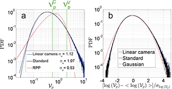
Fig. 3: (Color online) (a) PDFs of Voronoï cells areas  for the linear camera (blue line) and the standard measurements (black line) for
  . The red dashed line represents a RPP distribution. (b) Same comparison for the PDF, centred and reduced, of
  for the same parameters as before. The red dashed line represents a Gaussian distribution.
Download figure:
Standard imageFigure 4 shows, for all the carried experiments, the properties of Voronoï cells (figs. 4(a), (b)) and clusters geometry (figs. 4(c), (d)) obtained from the new analysis. Overall, these results are in very good agreement with those in the previous work using a standard analysis of images in [5]. Figures 4(a), (b) confirm, with the new approach, the diagnosis of clustering for all the datasets, with a robust quasi-lognormal distribution of Voronoï areas. The inset in fig. 4(b) shows the standard deviation  of normalized Voronoï areas, whose departure from the RPP value
  quantifies the level of clustering. The average value of
  from the new analysis is slightly larger, but still in good agreement with the value of 1.05 reported in [5]. PDFs of clusters area (fig. 4(c)) show a similar collapse as in [5] when normalized by the mean, with a clear peak around
  , although some scatter is visible for the tails of smallest areas. Similarly, fig. 4(d) shows cluster perimeters as a function of the squared root of its area, with a fractional behaviour of the exponent, identical to what was obtained with the classical analysis of images, evidencing the fractal nature of clusters. Altogether, these agreements validate the reconstruction procedure of the large-scale particle fields.

Fig. 4: (Color online) (a) PDFs of Voronoï cells areas  for the long reconstructed fields. The black dashed line represents a RPP distribution. (b) Same comparison for the PDF, centered and reduced, of
  . The black dashed line represents a Gaussian distribution. Inset: Stokes number dependence of
  . (c) PDF of the clusters area normalized with its mean value for the same cases. Inset: Stokes number dependence of the total mean area normalized with the dissipation length. (d) Clusters perimeter as a function of the squared root of its area for the experiment at
  .
.
Download figure:
Standard imageSuperclustering
We address the question of the clustering properties of clusters themselves. This is made possible from the new large-scale field reconstructed, which includes several tens of thousands of clusters, therefore allowing to study the collective properties of clusters.
The procedure to identify these structures is conceptually very simple: using the large-scale reconstructed fields, clusters are identified (fig. 2(e)) following the same thresholding procedure on normalized Voronoï areas PDF previsouly described. Then, the centres of clusters are defined as the center of mass of the constituting particles, weighted by the local concentration (which for each particle is given by the inverse of its Voronoï area), as represented in fig. 2(e). Once the centers of mass of the clusters are identified, Voronoï tessellations of cluster centers are computed (fig. 2(f)). We then compute the statistics of the areas of the resulting Voronoï cells, to diagnose (in the same way as for the particle themselves) the eventual presence of clustering for the center of clusters, which we call superclustering.
Figures 5(a), (b) represent the PDFs of  (the normalized Voronoï areas of cluster centers) and the PDFs of
  , centered and reduced, for all the studied parameters. The PDF of
  shows a clear departure from a random distribution, hence evidencing the presence of clustering of clusters. The inset of fig. 5(b) shows the dependence of the standard deviation of normalized Voronoï area,
  , with particles Stokes number (which we recall to be here directly related to the Reynolds number of the flow, as
  only varies because of the change in
  as
as  is varied). We find that
  remains almost constant for all sets (inset in fig. 5(b)). It is larger than the value of 0.53 expected for a random distribution (confirming the presence of clustering) and lower than the value obtained for the standard deviation of Voronoï areas of particles. The intensity of clustering, quantified by
  therefore diminishes when compared with the value of
  , which shows that superclustering (clustering of clusters) is less pronounced than simple clustering (clustering of particles). Interestingly, fig. 5(b) shows that superclustering maintains a quasi-lognormal distribution extremely similar to that observed for clusters. This quasi-lognormal behavior for Voronoï tesselations of particles has not been explained yet to our knowledge. We show here that this behavior is robust and prevails at the cluster level.
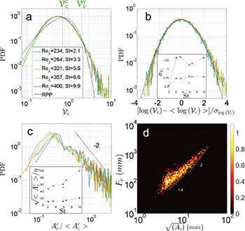
Fig. 5: (Color online) Same quantities as in fig. 4 but for superclustering analysis. In (a) and (b)  is the normalized area of Voronoï cells of cluster centers and
  and
and  the thresholds to define superclusters and supervoids. In (c) and (d)
  and
and  are, respectively, the area and the perimeters of superclusters. In (d) only
  is represented.
Download figure:
Standard imageFrom fig. 5(a) we determine the threshold  and define superclusters as connected regions of Voronoï cells such that
  (similarly, we can define supervoids as connected regions of Voronoï cells such that
  , although these will not be discussed here). Figure 2(g) shows an example of such superclusters. Figure 5(c) shows that the PDF of the area of superclusters
  has a shape almost identical to the PDF of
  for standard clusters (fig. 4(c)), with the same peak at
  . Besides, fig. 5(d) shows that superclusters have similar fractal trends than normal clusters. The mean area of superclusters is however (and naturally) larger than that of clusters, as shown in the inset of fig. 5(c): while the mean cluster size exhibits a weak dependence on experimental conditions, with a typical size of the order of 15η, the average size of superclusters increases markedly with particles Stokes number, reaching values as large as 100η (or 0.1L) for the experiments at the highest mean wind speed (corresponding to the highest values of St and
  investigated). It is important to note that superclusters can therefore have dimensions comparable to the field of view of original images
  , which emphasizes the importance of the proposed large-scale field reconstruction for the study of this phenomenon. To illustrate this, we have repeated the analysis of superclusters using the original images for
  . The resulting values of
  and
and  are shown with red markers in the inset of figs. 5(b), (c), showing that the standard analysis understimates both the level of superclustering (
 is very close to the RPP value) and the size of supeclusters. It is also important to note that although the reconstruction extends the streamwise dimension of the field of particles, the analysis is still limited in the vertical direction. It is therefore possible that even larger structures exist. As a matter of fact, we did identify elongated superclusters with a streamwise dimension exceeding 0.5L. This motivates future studies, with a larger vertical extended field of view, either by using an actual linear camera, or simply by rotating the camera sensor by 90°.
Discussion and conclusions
By emulating the acquisition of a linear camera and using Taylor hypothesis, several meters long fields of particles have been reconstructed, which allowed us to find the first evidence of superclustering of inertial particles in homogeneous isotropic turbulence. We have shown that superclusters present similar geometrical features (superclusters have quasi-lognormal PDF of Voronoï areas identical to clusters, superclusters have PDF of normalized area identical to clusters, with the same fractality signature), although superclustering is slightly weaker than clustering. This emphasizes the multi-scale nature of the spatial structuration of inertial particles in turbulence, without however a full scale invariance. It will be interesting to explore wether the superclustering features can be connected to the finding by Bec et al. [15], who showed that inertial particle distribution is non-uniform in the inertial range, but the coarse-grained mass distribution is not scale invariant. Further new analyses based on the large-scale reconstructed fields can be imagined and will be attempted in future studies. As already mentioned, by using an actual linear camera or rotating the camera sensor, we could optimize illumination conditions for a larger vertical field of view, and obtain more reliable estimations of superclusters geometry. In the present study we reconstructed long 2D fields from 1D (pixel lines) acquisitions normal to the freestream. The same idea can be extended to reconstruct full 3D particle fields from the acquisition of 2D cross-sections normal to the freestream which may give a simple way to investigate 3D properties of clustering. Further possible analyses also include the investigation of spatial correlation of particles concentration field, calculation of large-scale particle image velocimetry (PIV) velocity field (by reconstructing two large-scale particles fields using two different bands of pixels at two locations of the image, and cross-correlating these 2 fields for PIV calculations). Besides, one can also imagine computing the PIV not on usual square PIV cells, but on a PIV mesh defined based on the Voronoï cells, to better account for the inhomogeneity of particles seeding and to get estimates of velocities according to the belonging or not of particles to clusters, superclusters, voids, supervoids, etc. The estimation of such dynamical properties conditioned on clustering properties is of particular importance to shed light into collective mechanisms responsible for the preferential concentration and eventually also impacting, for instance, the settling velocity of particles within clusters, as observed by Aliseda et al. [16].
Acknowledgments
The authors gratefully acknowledge the valuable help with the experiments from Vincent Govart, Stephane Mercier and Laure Vignal. This work was supported by the French Agence Nationale pour la Recherche (project ANR-12-BS09-011-03) and the COST action on "Flowing Matter" (project MP1305).