
Amplitude-Frequency Analysis of Emotional Speech Using Transfer Learning and Classification of Spectrogram Images
Volume 3, Issue 4, Page No 363-371, 2018
Author’s Name: Margaret Lech1,a), Melissa Stolar1, Robert Bolia2, Michael Skinner2
View Affiliations
1School of Engineering, RMIT University, VIC 3000, Australia
2Defence Science and Technology Group, VIC 3207, Australia
a)Author to whom correspondence should be addressed. E-mail: margaret.lech@rmit.edu.au
Adv. Sci. Technol. Eng. Syst. J. 3(4), 363-371 (2018); ![]() DOI: 10.25046/aj030437
DOI: 10.25046/aj030437
Keywords: Speech processing, Emotion recognition, Deep neural networks

I am text block. Click edit button to change this text. Lorem ipsum dolor sit amet, consectetur adipiscing elit. Ut elit tellus, luctus nec ullamcorper mattis, pulvinar dapibus leo.
Export Citations
Automatic speech emotion recognition (SER) techniques based on acoustic analysis show high confusion between certain emotional categories. This study used an indirect approach to provide insights into the amplitude-frequency characteristics of different emotions in order to support the development of future, more efficiently differentiating SER methods. The analysis was carried out by transforming short 1-second blocks of speech into RGB or grey-scale images of spectrograms. The images were used to fine-tune a pre-trained image classification network to recognize emotions. Spectrogram representation on four different frequency scales – linear, melodic, equivalent rectangular bandwidth (ERB), and logarithmic – allowed observation of the effects of high, mid-high, mid-low and low frequency characteristics of speech, respectively. Whereas the use of either red (R), green (G) or blue (B) components of RGB images showed the importance of speech components with high, mid and low amplitude levels, respectively. Experiments conducted on the Berlin emotional speech (EMO-DB) data revealed the relative positions of seven emotional categories (anger, boredom, disgust, fear, joy, neutral and sadness) on the amplitude-frequency plane.
Received: 06 June 2018, Accepted: 03 August 2018, Published Online: 25 August 2018
1. Introduction
This paper is an extension of work originally presented in the 11th International Conference on Signal Processing and Communication Systems, ICSPCS’2017 [1]. The conference work introduced a new, efficient, real-time speech emotion recognition (SER) methodology. A demo of this application can be found on: (https://www.youtube.com/watch?v=cIsVGiFNJfE&t=41).
In this study, the method proposed in [1] was used for analytical purposes to determine how different emotional categories are coded into the amplitude-frequency characteristics of emotional speech. The underlying assumption was that, the accuracy of detecting a particular emotion depends on how many cues related to this emotion are given by the input speech features. By selecting acoustic speech features representing or emphasizing different frequency and amplitude values, and observing which emotions were best recognised, the study determined links between different emotions and corresponding amplitude-frequency characteristics of speech. In other words, features that lead to higher classification accuracy for a given emotion were thought to be highly representative of this emotion.
The search for the “best” or the most representative acoustic features has been one of the most important themes driving SER, as well as emotional speech synthesis studies [2]. In SER, this knowledge can improve differentiation between emotions, and in speech synthesis, it can lead to more natural sounding emotional speech. Despite extensive research, it is still unclear what the “best” features are, as it is uncertain how different emotions are coded into the time-varying amplitude-frequency characteristics of speech.
The remaining sections of the paper are organized as follows. Section 2 gives a brief review of related studies. Section 3 explains the methodology. The experiments and discussion of results are presented in Section 4, and Section 5 provides the conclusion.
2. Previous Works
Traditionally, the links between speech acoustics and emotions have been investigated by classifying emotional speech samples based on various low-level parameters, or groups of parameters, defined by models of speech production. Examples of low-level parameters include the fundamental frequency (F0) of the glottal wave, formant frequencies of the vocal filter, spectral energy of speech, and speech rate. The low-level features were later enriched by the addition of higher level derivatives and statistical functionals of the low-level parameters. The Munich Versatile and Fast Open-Source Audio Feature Extractor (openSMILE) [3] gives the current software standard, allowing for the calculation of over 6000 low- and high-level acoustic descriptors of speech. In [4] links between acoustic properties of speech and emotional processes in speakers performing a lexical decision task were investigated. Basic parameters such as F0, jitter and shimmer were found to be correlated with emotional intensity. The results indicated that acoustic properties of speech can be used to index emotional processes, and that characteristic differences in emotional intensity may modulate vocal expression of emotion. However, acoustic parameters characterizing different types of emotions were not investigated.
It has been often assumed, especially in earlier studies, that unlike facial expressions that convey qualitative differences between emotions (emotional valence), speech can only communicate emotional intensity (arousal) [5,6]. This assumption was shown to be incorrect by proving that judges are almost as accurate in inferring different emotions from speech as from facial expression [7,8]. As suggested in [6], it is possible that F0, energy, and rate may be most indicative of arousal while qualitative, valence differences may have a stronger impact on source and articulation characteristics. One of the tables presented in [8] showed how selected acoustic speech parameters vary with different emotional categories. Namely, speech intensity, mean, variability and range of F0, sentence contours, high-frequency energy, and articulation rate have been compared across six emotional states (stress, anger/rage, fear/panic, sadness, joy/elation, and boredom). An investigation described in [9] shows links between emotions and prosody features including intonation, speaking rate and signal energy. Correlation between naturally expressed anger and despondency, and various acoustic cues of the speech signal of 64 call centre customers was analysed in [10]. It was found that anger was characterized by a rise of F0 and speech amplitude, whereas despondency by a decreased F0 and syllable rate. Teager energy operator (TEO) parameters [11-13], which simultaneously estimate the instantaneous energy and frequency changes of speech signals, have been shown to be effective in the classification of speech under stress [14,15] and in automatic SER [16]. It was suggested that the high effectiveness of these parameters is due to their sensitivity to the acoustic effects caused by a nonlinear air flow and the formation of vortices in the vicinity of the vocal folds. A discussion of the links between emotions and some of the basic acoustic features including F0, formants, vocal tract cross-section, mel-frequency cepstral coefficients (MFCCs) and TEO features, as well as the intensity of the speech signal and the speech rate can be found in [13]. The high velocity of air moving through the glottis and causing vocal fold vibration was found to be indicative for music-like speech such as joy or surprise while, low velocity was an indicator of harsher styles such as anger or disgust [17]. Identification of the “best” frequency sub-bands of the power spectrum for the classification of different emotions has not been conclusive. A number of studies [18-20] have indicated high importance of the low frequency band ranging from 0 to 1.5 kHz for speech emotions, whereas [21] pointed to the high frequency range (above 1.5 kHz). In He [16] discriminative powers of different frequency bands were examined. It was found that the largest diversity between energy contributions from different emotions occurs in the low frequency range of 0-250 Hz and the high frequency range of 2.5-4 kHz. The middle range of 250 Hz to 2.5 kHz did not show clear differences between emotions. Some of the most often used parameters in speech classification across different databases and languages are the MFCCs [22]. In general, MFCCs are thought to give good representation of the speech signal by considering frequency response characteristics of the human auditory system. However, applications of MFCCs into the SER task have shown relatively poor results [14,16,21,23]. The log-frequency power coefficients (LFPCs) calculated within critical bands of the human auditory system [24] were found to outperform the MFCCs [21]. Experiments presented in [16] examined and ranked 68 different low and high-level features for emotion recognition from natural (non-acted) speech. TEO parameters estimated within perceptual wavelet packet frequency bands (TEO-PWP), as well as the area under the speech energy envelope (AUSEE), have been found to produce the highest performance in both natural emotion and stress recognition.
As shown in the above few examples of the very rich research field, the task of finding links between categorical emotions and acoustic speech parameters has been particularly challenging due to inconsistencies between studies, which include the ways emotions are evoked in speakers (natural, acted, induced), types of emotional labels (different emotional categories or arousal/valence) and types of acoustic speech parameters [8,12,25]. To deal with these difficulties, current trends in automatic speech emotion recognition (SER) are shifting away from learning differences between individual low- or high-level parameters, and moving towards using speech spectrograms that capture the entire time-evolution of emotional acoustics in the form of two-dimensional, time-frequency, spectral magnitude arrays.
Deep neural network structures have been trained to efficiently classify speech spectrograms to recognize different emotional categories [26][33]. Although this methodology is very powerful, the current state-of-the-art results indicate that there is still room for improvement. In particular, the inter-emotional confusion tables show high levels of misclassification between neutral and dysphoric [16], neutral and boredom [34], and joy and anger [16],[34]. Systems designed with prior knowledge of emotional cues have been shown in the past to be particularly effective in increasing the overall SER accuracy. In [35][36] for example, a saliency analysis was applied to speech spectrograms to determine regions of the time-frequency plane that provide the most important emotional cues.
Application of these regions as inputs to a Convolutional Neural Network (CNN) led to high SER accuracy, however, the saliency analysis had a time-varying character and involved very high computational cost. This study offers a more computationally efficient approach to finding what parts of the amplitude-frequency plane carry the most important cues for different emotions. It is expected that the knowledge of the amplitude-frequency characteristics of individual emotions will facilitate future designs of more efficient SER systems with reduced inter-class confusion.
Table 1: Speech and image data description.
| Emotion | No. of speech samples (utterances) | Total duration of speech samples [sec] | No. of generated spectrogram images (RGB or Grey-Scale) |
| Anger | 129 | 335 | 27220 |
| Boredom | 79 | 220 | 18125 |
| Disgust | 38 | 127 | 11010 |
| Fear | 55 | 123 | 5463 |
| Joy | 58 | 152 | 12400 |
| Neutral | 78 | 184 | 14590 |
| Sadness | 53 | 210 | 18455 |
| TOTAL | 390 | 1207 | 111425 |
3. Method
3.1. Speech Data
The study was based on the EMO-DB database [37] that is routinely used in evaluations of SER systems. It contains speech recordings collected from 10 professional actors (5 male and 5 female) speaking in fluent German. Each actor simulated 7 emotions (anger, joy, sadness, fear, disgust, boredom and neutral speech) while pronouncing 10 different fixed-text utterances consisting of single sentences with linguistically neutral contents. Each actor pronounced each utterance with a different emotion, however in some cases the speakers provided more than one version of the same utterance. Table 1 shows the numbers and total duration of available speech samples (pronounced utterances) for each emotion. The original recordings were validated using listening tests conducted by 10 assessors; details can be found in [37]. Only speech samples that scored recognition rates greater than 80% were used in this study. The sampling rate was 16 kHz, giving 8 kHz speech bandwidth. Despite more recent developments of emotional speech datasets, the EMO-DB remains one of the best and most widely used standards for testing and evaluating SER systems. The important strength of the EMO-DB is that it offers a good representation of gender and emotional classes. The main disadvantage is that the emotions appear to be acted in a strong way, which in some cases may be considered as unnatural.
3.2. SER Using Transfer Learning and Images of Spectrograms
Existing state-of-the-art SER methods apply deep Convolutional Neural Networks (CNNs) trained on spectral magnitude arrays of speech spectrograms [26-29]. To achieve high accuracy, complex CNN structures must be trained on a very large number (in the order of millions) of labelled spectrograms. This method (known as “fresh training”) is computationally intense, time consuming and requires large graphic processing units (GPUs).
At present the availability of large datasets of emotionally labelled speech is limited. On the other hand, in many cases, close to the state-of-the-art results can be achieved using a much simpler process of transfer learning. In transfer learning a small, problem-specific data set is used to fine-tune an existing network that has been already pre-trained on a very large amount of more general data.
Table 2: Fine-tuning parameters for AlexNet (Matlab version 2017b)
| Parameter | Value |
| Minibatch size | 128 |
| Maximum number of epochs | 5 |
| Weight decay | 0.0001 |
| Initial learning rate | 0.0001 |
| Weight learn rate factor | 20 |
| Bias learn rate factor | 20 |
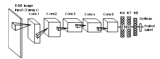 Figure 1. Structure of AlexNet. The input consists of 3 arrays (3 input channels). Feature extraction is performed by 5 convolutional layers (Conv1-5), and classification by 3 fully-connected layers (fc5-8). The output is given in the form of soft labels indicating probability of each class.
The current study applied transfer learning to a pre-trained, general-purpose image classification network known as AlexNet [38], with inputs given as images (not magnitude arrays) of speech spectrograms. AlexNet has been trained on over 1.2 million images from the ImageNet [39] data representing 1000 classes. As shown in Figure 1, AlexNet is a CNN [40] that consists of a 3-channel input layer followed by five convolutional layers (Conv1-Conv5) along with max-pooling and normalization layers, and three fully connected layers (fc6-fc8). The output from the last layer is passed through the normalized exponential Softmax function [41] that maps a vector of real values (that sum to 1) into the range [0, 1]. These values represent the probabilities of each object class. In the experiments described here, the final classification label was given by the most probable class (emotion). The fine tuning of AlexNet was performed within the Matlab (version 2017b) programming framework [42]. The network was optimized using stochastic gradient descent with momentum (SGDM) and L2 regularization factor applied to minimize the cross-entropy loss function. Table 2 provides values of the tuning parameters. Given this choice of parameters, the fine-tuning process changed mostly the final, fully connected (data-dependent) layers of the network leaving the initial (data-independent) layers almost intact.
Despite the fact that in recent years AlexNet has been rivalled by newer, significantly more complex and more data demanding networks, the pre-trained structure is still of great value, as it provides a good compromise between data requirements, network simplicity and high performance. Informal tests on more complex networks such as the residual network ResNet-50, the Oxford Visual Geometry Group networks VGG-16 and VGG-19, and the GoogleLeNet have shown that for a given outcome, the training time needed by the larger networks was significantly longer than for AlexNet. It could also imply that a larger dataset may be needed, but it would have to be confirmed by formal testing.
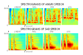 Figure 2. Examples of RGB images of speech spectrograms for the same sentence pronounced with sadness and anger, and depicted on four different frequency scales linear, mel, ERB and log. The linear scale represents the high frequency details, mel scale-the mid-high frequency details, ERB – the mid-low frequency details and log – the low frequency details.
3.3. Generation of Spectrogram Images
The amplitude-frequency analysis of the characteristics of emotional speech was achieved by analyzing the SER results given by different forms of features (i.e. spectrogram images representing speech signals. The SER was performed by applying transfer learning to the pre-trained AlexNet with input arrays given as RGB or grey-scale images depicting speech spectrograms [1] (see Figure 4). To preserve the feasibility of real-time SER [1,26,27], the features were generated on a frame-by-frame basis, and no utterance based parameters were calculated. Since the emotional labels for the EMO-DB data were given for entire utterances, the emotional label for each frame was assumed to be the same as the label of the utterance from which it was extracted. Short-time Fourier transform spectrograms were computed for 1-second blocks of speech waveforms using Hamming window frames of length 25 milliseconds with 12.5 milliseconds of overlap between frames. Short silence intervals occurring within sentences were kept intact. The calculations were performed using the Matlab Voicebox spgrambw procedure [43], which generated magnitude spectrogram arrays of size 257 x 259 for the frequency and time dimensions, respectively. The stride between subsequent 1-second blocks was 10 milliseconds. Table 1 shows the numbers of images generated from the available speech data.
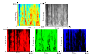 Figure 3. An example of the RGB, grey-scale, R, G and B spectrogram images for the same speech sample of emotionally neutral speech. The R components emphasizes high-amplitude details, the G component – the mid amplitude details and the B component – the low-amplitude details.
The experiments investigated and compared four frequency scales of speech spectrograms: linear, melodic (mel) [44], equivalent rectangular bandwidth (ERB) [45] and logarithmic (log) [46]. While the alternative frequency scales were applied along the vertical axis of the spectrograms from 0 to 8 kHz, the horizontal time scale was in all cases linear spanning the time range of 0 to 1 second. The dynamic range of spectral magnitudes was normalized from -130 dB to -22 dB, representing the respective minimum (Min) and maximum (Max) magnitude values. These values were calculated for magnitude spectrograms over the entire database. The magnitude spectrograms were transformed into RGB or grey-scale images. The RGB images were generated with the Matlab “jet” colormap [47,48] containing 64 default colors. After downsampling to 227 x 227 pixels (using the Matlab imresize command), the spectrogram images provided input arrays to AlexNet (Figure 4). More details on the AlexNet input arrangements are given in Section 4.
3.4. Frequency Representation by Different Scales of Spectrogram Images
Four different frequency scales (linear, mel, ERB and log) [49] were applied when generating the spectrogram images in order to visually emphasize different frequency ranges. Figure 2 shows examples of spectrograms for the same sentence pronounced with sad and angry emotion plotted on four different frequency scales: linear, mel, ERB and log [49]. This order of scales corresponds to the process of gradually “zooming into” the lower frequency range features (about 0 to 2 kHz), and at the same time “zooming out” of the higher frequency range features (about 2 kHz to 8 kHz) features. Therefore, the application of different frequency scales effectively provided the network with either more- or less-detailed information about the lower or upper range of the frequency spectrum.
Thus, the linear scale emphasized details of the high-frequency (6-8 kHz) components of speech characterizing unvoiced consonants. The mel and ERB scales provided details of the mid-high (4-6 kHz) and mid-low (2-4 kHz) ranges, respectively (characteristic to both voiced and unvoiced speech), and the log scale provided the most details of the low-frequency (0.02-2 kHz) range (important for vowels and voiced consonants).
3.5. Amplitude Representation by R, G and B Images of Spectrograms
While the RGB images of spectrograms used in the speech classification gave visual representations of the time-frequency decomposition of speech signals, each of the R, G and B color components emphasized a different range of speech spectral amplitude values. As shown in Figure 3, the R component gave greatest intensity of the red color for high spectral amplitude levels, thus emphasizing details of the high-amplitude spectral components of speech (e.g. vowels and voiced consonants). The B component gave greatest intensity of the blue color for lower amplitudes, and therefore it emphasized details of the low-amplitude spectral components of speech (e.g. unvoiced consonants) and gaps between speech. Similarly, the G component emphasized details of the mid-range spectral amplitude components (both voiced and unvoiced).
3.6. Experimental Setup
A 5-fold cross-validation technique was used with 80% of the data distributed for the fine tuning, and 20% for the testing of AlexNet. All experiments were speaker- and gender-independent. The experimental framework is illustrated in Figure 4. Three different experiments, each having different data arrangements for the three input channels of the AlexNet were conducted as follows:
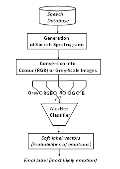 Figure 4. Framework diagram for the amplitude-frequency analysis of emotional speech.
- Experiment 1. To investigate the performance of the color RGB images of spectrograms on average and across emotions.
AlexNet input: A different color-component array (R, G and B) was given as an input to each of the 3 input channels. The same process was repeated for four different frequency scales of spectrograms.
- Experiment 2. To investigate how the grey-scale image representation of spectrograms performs on average and across emotions.
AlexNet input: Identical copies of grey-scale image arrays were given as inputs to each of the 3 input channels. It was repeated for four different frequency scales of spectrograms.
- Experiment 3. To investigate how each of the individual color components (R, G or B) performs on average and across emotions.
AlexNet input: Identical copies of arrays representing the same color component were provided as inputs to each of the 3 input channels. It was repeated for four different frequency scales of spectrograms.
In contrast with the common practice of duplicating the information provided to the network channels [29], the first experiment provided more meaningful and complimentary information to each of the three processing channels of the neural network.
3.7. SER Performance Measures
The emotion classification performance was assessed using standard measures applied in SER tasks. It included accuracy, F-score, precision and recall [50][51] given by (1)-(4) respectively, and calculated separately for each emotion.
 Where, tp and tn denoted numbers of true positive and true negative classification outcomes, while fp and fn denoted numbers of false positive and false negative classification outcomes, respectively.
To reflect the fact that the emotional classes were unbalanced, the weighted average accuracy and F-score were estimated as:
![]() Where denoted either accuracy or F-score for the ith class ( ) given as (1) or (2) respectively. The values of |ci| denoted class sizes and N was the number of classes.
Where denoted either accuracy or F-score for the ith class ( ) given as (1) or (2) respectively. The values of |ci| denoted class sizes and N was the number of classes.
4. Results and Discussion
The outcomes of the three SER experiments showed what type of input to AlexNet provided the most efficient training and emotion recognition results. By doing so, indirect insights into the spectral amplitude-frequency characteristics of different emotions were gained. It was achieved through both the application of different frequency scales of spectrograms that visually emphasized details of different frequency ranges, as well as the use of different color components that emphasized different spectral amplitude ranges of speech.
4.1. Comparison between Classification Performance of RGB, Grey-Scale and R, G and B Components
On average, the RGB images outperformed the individual color components and grey-scale images, giving the highest average classification accuracy and F-scores for all frequency scales (Figure 5). Both the RGB and grey-scale images achieved highest performance with the mel frequency scale. The largest difference between RGB and grey-scale images was observed for
the ERB and log scales (about 2%). For the other scales, the difference was only about 1% showing that the high frequency details depicted by the ERB and log scales were likely to be clearly depicted by the color RGB images, and to some extend blurred by the grey-scale images.
In addition, Figure 5 shows that the best performing single-color component was green (G) followed by red (R), and the worse performing was blue (B). It indicates that the mid-amplitude spectral components of speech are likely to be the most important for the differentiation between emotions. The low-amplitude components play a less important role, since they predominantly represent unvoiced speech and gaps of silence between words. For the R color-component, which emphasized high-amplitude speech components, the highest performance was given by the mel scale, which provided a detailed view of the mid-high frequency range. Therefore, the high-amplitude emotional cues appeared to be linked mostly to the mid-high frequency speech components (which amongst other things contain information about the harmonics of the glottal wave fundamental frequency (F0) and the higher formants of the vocal tract).
For the G color-component, the ERB scale, which reveals the mid-low frequency details of speech, was the best performing. This shows that the mid-amplitude emotional cues could be linked to the mid-low-frequency speech components (low harmonics of F0 and low formants). Finally, for the B color-component, the linear scale provided the best performance. This indicates that the low-amplitude emotional cues are predominantly linked to the higher frequency components of speech, such as unvoiced consonants, higher formants and higher harmonics of F0, as well as additional harmonic components generated due to the nonlinear air flow and vortex formation in the vicinity of the glottal folds [14].
4.2. Comparison between RGB, Grey-Scale and R, G and B Components across Different Emotions and Frequency Scales.
To analyze the performance of different spectrogram representations across different emotions, precision-recall graphs shown in Figures 6 and 7 were made. When using this representation, the classification aim was to achieve results that were close to the diagonal line of equal precision and recall values, and as close as possible to the top right corner showing the maximum values of these two parameters. Taking this into account, anger was detected with the highest precision/recall scores by the R-components using the ERB-scale, indicating that the anger cues are most likely to be encoded into the high amplitude and medium-low frequency components of speech.
Disgust was most efficiently detected by the RGB images using the logarithmic frequency scale, which points to the low frequency speech components spanning all amplitude values as carriers of this emotion. Joy was coded the same way as anger into the medium-low frequency and high amplitude components, as it was best detected by the R-image components and the ERB scale.
Boredom showed a distinctly different pattern by being best detected by the mel-scale and G-images. This means that boredom was coded into the medium-high frequencies and medium range amplitudes of speech.
Fear was also distinctly different by being best detected by the mel-frequency scale and grey-scale images. This points to the medium-high frequency range and all amplitude values of speech as carriers of this emotion.
Sadness gave the best performance for the mel-scale and RGB images, showing that like fear, it was coded into mid-high frequencies and all amplitude values of speech.
 Figure 5. Average weighted classification accuracy (a) and F-score (b) using different frequency scales.
Finally, the emotionally neutral speech was best detected by the ERB scale and RGB images. Therefore, it was likely to be coded into the medium-low frequencies across all amplitudes values of speech. These observations are summarized in Table 3.
4.3. Statistical Significance Analysis
As shown in the above examples, different forms of spectrogram image representation lead to different classification outcomes. To find out which of the observed differences were statistically significant, one-way ANOVA analysis with Bonferroni correction was conducted using the SPSS package. The results comparing the average accuracy values obtained during SER are presented in Table 4. In 5 out of 10 possible pairs of spectrogram image representation, the differences were found to be statistically significant. Namely, the B components were significantly different compared to all other types of images, the R components were different compared to the RGB and B components, and finally the G components were significantly different only when compared to the B components. On average, there was no significant difference between the RGB images and G image-components. The least significant differences were obtained for the grey-scale images compared to the G image-components. This means that, in terms of the classification accuracy, the grey-scale representation appears to be very close to the G images – both giving good visual information of the mid-amplitude components of speech, which, as previously discussed, were the most important carriers of emotional cues.
 Figure 6. Precision vs. recall using different frequency scales for anger, disgust, joy and boredom. The markers shapes indicate the frequency scale, while their colors indicate types of spectrogram images.
4.4. Distribution of Categorical Emotions on the Amplitude-Frequency Plane
Given the performance analysis of the separate R, G and B images across emotions and frequency scales summarized in Table 3, Figure 8 was made to show the relative positions of seven emotional states of the EMO-DB database on the amplitude-frequency plane. The graph predicts high possibility of confusion in the differentiation between joy and anger, which is consistent with [16,34], as well as, between sadness and fear. Much higher precision/recall scores for anger in Figure 6 suggested that joy was frequently mistaken for anger. Similarly, higher precision/recall scores for sadness in Figure 7 suggested that fear was frequently mistaken for sadness. As expected, neutral speech took central position in relation to other emotions. Both joy and anger were acted in the EMO-DB data by rising the voice level, which is consistent with [10]. Disgust on the other hand, was achieved by variation of the fundamental frequency (F0) and the first formants. Sadness and fear were placed across all amplitudes, but at relatively high frequencies, which could be due to a large number of unvoiced consonants that can be heard when listening to the recordings.
 Figure 7. Precision vs. recall using different frequency scales for fear, sadness, and neutral emotional state. The markers shapes indicate the frequency scale, while their colors indicate types of spectrogram images.
Table 3: Amplitude-frequency characteristics of categorical emotions. The total frequency range was 8 kHz, and the total amplitude range was 108 dB.
| Emotion |
Best Freq.Scale
|
Best Freq Range |
Best CNN Input (3 channels) |
ImportantAmplit. Range | ||
| Ch1 | Ch2 | Ch3 | ||||
| Anger | ERB |
Medium-Low
|
R | R | R | High |
| Disgust | LOG |
Low (0.02-2kHz) |
R | G | B |
All
|
| Joy | ERB |
Medium-Low (2-4kHz) |
R | R | R |
High
|
| Boredom | MEL |
Medium-High (4-6kHz) |
G | G | G | Medium |
| Fear | MEL |
Medium-High (4-6kHz) |
R or Greyscale | G or Greyscale | B or Greyscale |
All
|
| Sadness | MEL |
Medium-High (4-6kHz) |
R | G | B |
All
|
| Neutral | ERB |
Medium-Low (2-4kHz) |
R | G | B |
All
|
Table 4: Statistical significance (p) values obtained when comparing average accuracy of SER based on different types of spectrogram images.
| p-values for one-way ANOVA with post-hoc Bonferroni correction, confidence interval: 95%, Bonferroni alpha: 0.05 | |||||
| RGB | Grey | R | G | B | |
| RGB | – | 0.997 | 0.009 | 0.868 | 0.000 |
| Grey | 0.997 | – | 0.315 | 1.000 | 0.000 |
| R | 0.009 | 0.315 | – | 0.367 | 0.019 |
| G | 0.868 | 1.000 | 0.367 | – | 0.000 |
| B | 0.000 | 0.000 | 0.019 | 0.000 | – |
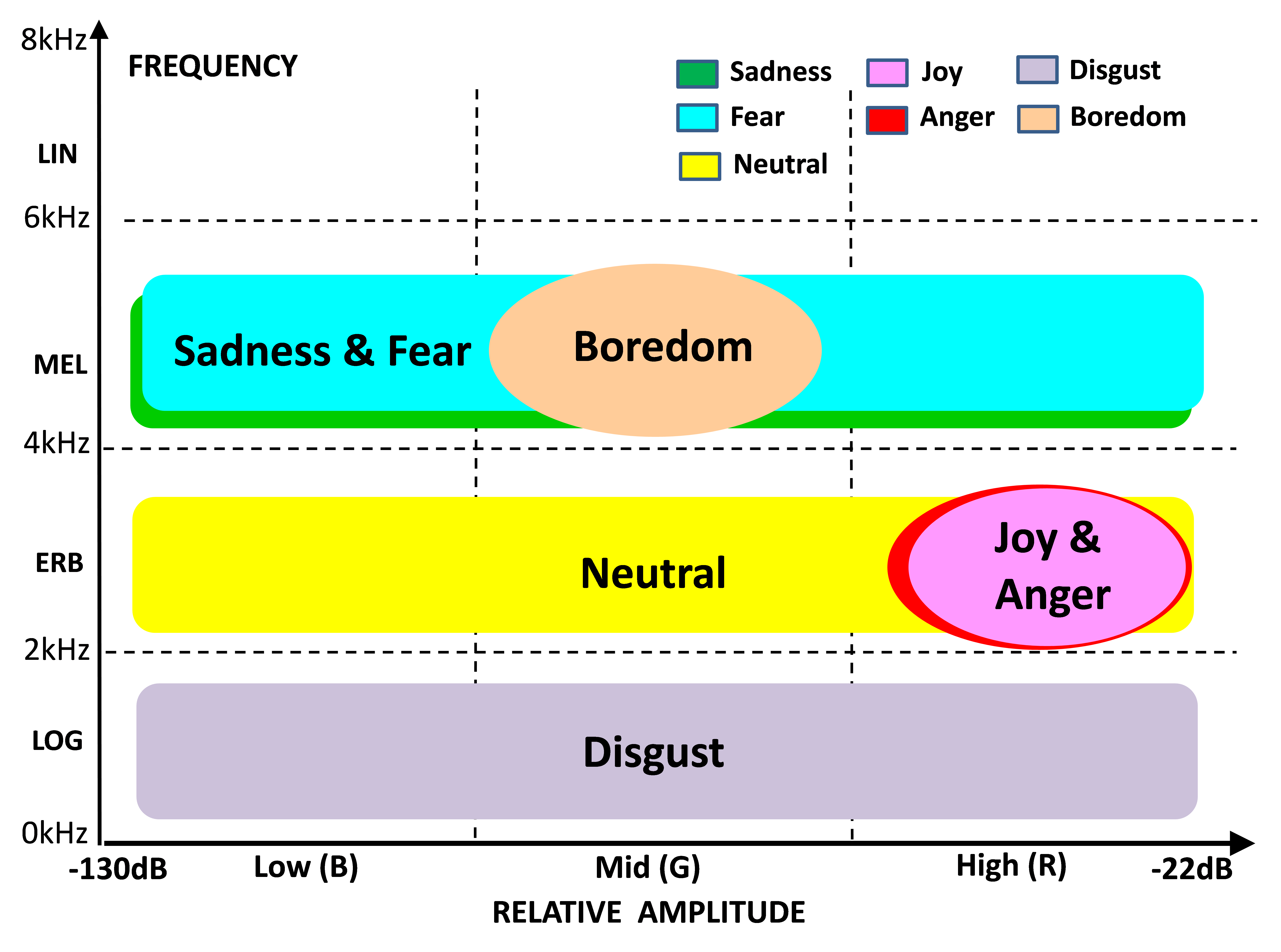 Figure 8. Relative positions of categorical emotions on the amplitude-frequency plane representing acoustic characteristics of emotional speech. These results were obtained using the EMO-DB database
Finally, boredom was localized at mid amplitude levels and high frequencies, which is consistent with very flat, monotonous speech having shallow amplitude modulation. In general, these insights confirmed the expectations, and the fact that they have been generated through machine learning shows that the analysis was valid and consistent with linguistic knowledge. From the perspective of machine learning these insights have direct practical consequences. It is likely that in the future, the SER training process can be enhanced by an adaptive choice of the input features to the network based on optimal configurations given in Table 4.
5. Conclusion
An automatic SER technique based on transfer learning and spectral image classification has been applied to perform an indirect analysis of the amplitude-frequency characteristics of the seven emotional categories represented by the EMO-DB database. Spectrogram images generated on different frequency-scales emphasized different frequency ranges of speech signals, while different color components of the RGB images of spectrograms indicated different values of spectral amplitudes. The analysis provided insights into the amplitude-frequency characteristics of emotional speech. Areas of the amplitude-frequency plane containing cues for different emotions were identified. One of the major limitations of this study is that, the findings apply to acted emotional speech, and only one language (German) was tested. Future works will investigate if the outcomes of the current study are consistent with natural (non-acted) emotional speech, and if they apply across different languages. In addition, factors allowing to efficiently differentiate between highly confused emotions such as for example anger and joy or sadness and fear will be investigated.
Conflict of Interest
The authors declare no conflict of interest.
Acknowledgment
This research was supported by the Defence Science Technology Institute and the Defence Science and Technology Group through its Strategic Research Initiative on Trusted Autonomous Systems, and the Air Force Office of Scientific Research and the Office of Naval Research Global under award number FA2386-17-1-0095.
- M.N. Stolar, M. Lech, R.S. Bolia, and M. Skinner, “Real Time Speech Emotion Recognition Using RGB Image Classification and Transfer Learning”, ICSPCS 2017, 13-16 December 2017, Surfers Paradise, Australia, pp.1-6.
- M. Schröder, “Emotional Speech Synthesis: A Review”, Seventh European Conference on Speech Communication and Technology, Aalborg, Denmark September 3-7, 2001, pp. 1-4.
- F. Eyben, F. Weninger, M. Woellmer, and B. Schuller, “The Munich Versatile and Fast Open-Source Audio Feature Extractor”, [Online] Accessed on: Feb 15 2018, Available: https://audeering.com/technology/opensmile/
- J.A Bachorovski and M.J. Owren, Vocal expression of emotion: Acoistic properties of speech are associated with emotional intensity and context”, Psychological Science, 1995, 6(4), pp. 219-224.
- K.R. Scherer, “Non-linguistic indicators of emotion and psychopathology”. In: Izard, C.E. (Ed.), Emotions in Personality and Psychopathology. Plenum Press, New York, 1979, pp. 495–529.
- K.R. Scherer, 1986. Vocal affect expression: A review and a model for future research. Psychol. Bull. 99 (2), 143–165.
- T. Johnstone and K.R. Scherer, 2000. Vocal communication of emotion. In: Lewis, M., Haviland, J. (Eds.), Handbook
- K.R. Scherer, “Vocal communication of emotion: A review of research paradigms”, Speech Communication 2003, (40), pp. 227–256.
- J. Tao, and Y. Kang, “Features importance analysis for emotional speech classification”, International Conference on Affective Computing and Intelligent Interaction, ACII 2005: Affective Computing and Intelligent Interaction pp 449-457.
- M. Forsell, “Acoustic Correlates of Perceived Emotions in Speech”, Master’s Thesis in Speech Communication, School of Media Technology, Royal Institute of Technology, Stockholm, Sweden 2007.
- Maragos, P., J.F. Kaiser, and T.F. Quatieri, Energy separation in signal modulations with application to speech analysis. Signal Processing, IEEE Transactions on, 1993. 41(10): p. 3024-3051.
- D. Ververidis and C. Kotropoulos, Emotional speech recognition: resources, features and methods “, Speech Communication, Volume 48, Issue 9, September 2006, Pages 1162-118.
- D. Ververidis, and C. Kotropoulos, Emotional speech recognition: Resources, features, and methods. Speech Communication, 2006. 48(9): p. 1162-1181.
- G. J. Zhou, J. H. L. Hansen, and J. F. Kaiser, “Nonlinear feature based classification of speech under stress,” IEEE Trans. Speech Audio Process., vol. 9, no. 3, pp. 201–216, Mar. 2001.
- L. He, M. Lech, N. Maddage, and N. Allen, “Stress detection using speech spectrograms and sigma-pi neuron units”, iCBBE, ICNC’09-FSKD’09, 14-16 August 2009 Tianjin, China, pp. 260-264.
- L. He, “Stress and emotion recognition in natural speech in the work and family environments”, PhD Thesis, RMIT University, Australia, 2010.
- A. Nogueiras, J.B. Marino, A. Moreno, and A. Bonafonte,, 2001. Speech emotion recognition using hidden Markov models. In: Proc. European Conf. on Speech Communication and Technology (Eurospeech 2001), Denmark.
- F.J. Tolkmitt and K.R. Scherer, 1986. Effect of experimentally induced stress on vocal parameters. J. Exp. Psychol. [Hum. Percept.] 12 (3), 302–313.
- R. Banse and K.R. Scherer, 1996. Acoustic profiles in vocal emotion expression. J. Pers. Soc. Psychol. 70 (3), 614–636.
- D.J. France, R.G. Shiavi, S. Silverman, M. Silverman, and M. Wilkes, 2000. Acoustical properties of speech as indicators of depression and suicidal risk. IEEE Trans. Biomed. Eng. 7, 829–837.
- T. L. Nwe, S.W. Foo, and L.C. De Silva, 2003. Speech emotion recognition using hidden Markov models. Speech Comm. 41, 603–623.
- S.B. Davis and P. Mermelstein (1980), “Comparison of parametric representations for monosyllabic word recognition in continuously spoken sentences.” IEEE Transactions on ASSP 28: 357–366.
- L. He, M. Lech, and N.B. Allen, “On the Importance of Glottal Flow Spectral Energy for the Recognition”, Interspeech 2019, pp. 2346-2349.
- B.C.J. Moore and B.R. Glasberg (1983) “Suggested formulae for calculating auditory-filter bandwidths and excitation patterns” The Journal of the Acoustical Society of America (JASA) 1983, 74, pp. 750-753.
- R. Cowie, E. Douglas-Cowie, N. Tsapatsoulis, G. Votsis, S. Kollias, W. Fellenz, and J.G. Taylor, “Emotion recognition in human-computer interaction”, 2001 IEEE Signal Processing Magazine, 2001, Volume 18, Issue 1, pp. 32-80.
- H. Fayek, M. Lech, and L. Cavedon, “Towards real-time speech emotion recognition using deep neural networks”, ICSPCS, 14-16 December 2015, Cairns, Australia, pp. 1-6.
- H.M. Fayek, M. Lech and L. Cavedon L, “Evaluating deep learning architectures for speech emotion recognition”, Neural Networks, March 2017, Special Issue 21, pp. 1-11.
- Z. Huang M. Dong, Q. Mao, and Y. Zhan, “Speech emotion recognition using CNN”, ACM 2014, November 3-7, 2014, Orlando Florida, USA, pp. 801-804.
- W. Lim, D. Jang, and T. Lee, “Speech emotion recognition using convolutional and recurrent neural networks”. In Proceedings of the Signal and Information Processing Association Annual Summit and Conference, Jeju, Korea, December 2016, pp. 1–4.
- Q. Mao, M Dong, Z.Huang and Y. Zhan, “Learning salient features for speech emotion recognition using convolutional neural networks”, IEEE Transactions on Multimedia, 16(8), December 2014, pp. 2203-2213.
- S. Prasomphan and K. Mongkut, “Use of neural network classifier for detecting human emotion via speech spectrogram”, The 3rd IIAE International Conference on Intelligent Systems and Image Processing 2015, pp. 294-298.
- S. Mirsamadi, E. Barsoum, and C. Zhang, “Automatic speech emotion recognition using recurrent neural networks with local attention”, Acoustics, Speech and Signal Processing (ICASSP), 2017 IEEE International Conference on, 5-9 March 2017, New Orleans, LA, USA, pp. 2227 – 2231.
- A.M. Badshah, J. Ahmad, N. Rahim, and S.W. Baik, “Speech emotion recognition from spectrograms with deep convolutional neural network”, Platform Technology and Service (PlatCon), 2017 International Conference on, 13-15 Feb. 2017, Busan, South Korea, pp. 1-5.
- M. Stolar, “Acoustic and conversational speech analysis of depressed adolescents and their parents”, 2017, PhD Thesis, RMIT University.
- Z. Huang M. Dong, Q. Mao, and Y. Zhan, “Speech emotion recognition using CNN”, ACM 2014, November 3-7, 2014, Orlando Florida, USA, pp. 801-804.
- Q. Mao, M Dong, Z.Huang and Y. Zhan, “Learning salient features for speech emotion recognition using convolutional neural networks”, IEEE Transactions on Multimedia, 16(8), December 2014, pp. 2203-2213.
- F. Burkhardt, A. Paeschke, M. Rolfes, W. Sendlmeier, and B. Weiss, “A database of German emotional speech”, Interspeech 2005, 4-8 September 2005, Lisbon, Portugal pp. 1-4.
- A. Krizhevsky, I. Sutskever, and G.E. Hinton, “Imagenet classification with deep convolutional neural networks”, Advances in Neural Information Processing Systems, 2012, pp.1097-1105.
- IMAGENET, Stanford Vision Lab, Stanford University, Princeton University 2016 Accessed on: Jan 14 2018 [Online], Available: http://www.image-net.org/
- Y. LeCun, Y. Bengio, and G. Hinton, “Deep learning”, Nature, 2015, 521, pp. 436-444.
- C.M. Bishop, “Pattern Recognition and Machine Learning”, Springer 2006.
- MathWorks documentation: Alexnet, Accessed on: Jan 14 2018, [Online], Available:
https://au.mathworks.com/help/nnet/ref/alexnet.html?requestedDomain=true - Voicebox, Description of spgrambw Accessed on: Jan 14 2018, [Online], Available:
http://www.ee.ic.ac.uk/hp/staff/dmb/voicebox/doc/voicebox/spgrambw.html - S.S. Stevens and J. Volkman, “The relation of pitch to frequency: A revised scale” The American Journal of Psychology 1940, 53, pp. 329-353.
- B.C.J. Moore and B.R. Glasberg (1983) “Suggested formulae for calculating auditory-filter bandwidths and excitation patterns” The Journal of the Acoustical Society of America (JASA) 1983, 74, pp. 750-753.
- H. Traunmüller and A. Eriksson, “The perceptual evaluation of F0-excursions in speech as evidenced in liveliness estimations” The Journal of the Acoustical Society of America (JASA), 1995, 97: pp. 1905 – 1915.
- MathWorks; Documentation Jet; Jet colormap array, Accessed on: Jan 14 2018, [Online], Available:
https://au.mathworks.com/help/matlab/ref/jet.html?requestedDomain=www.mathworks.com - Matlab Documentation Colormaps: Accessed on: Jan 14 2018, [Online], Available:
https://au.mathworks.com/help/matlab/colors-1.html - B. Moore, “An Introduction to the Psychology of Hearing”, Sixth Edition, Emerald Group Publishing Limited, 2012.
- B. Schuller, S. Steidl, and A. Batliner, “The Interspeech 2009 emotion challenge”. In Proceedings of Interspeech 2009, pp. 312–315.
- B. Schuller, S. Steidl, A. Batliner, F Schiel and J Krajewski, “The Interspeech 2011 speaker state challenge”. In Proceedings of Interspeech 2011, August 2011, pp.1-4.