1. Introduction

For many reasons, such as people, productivity, management and working environment; the robots gradually replace the people to carry out the tasks flexibly, accurately and safely. The tasks such as assembling and disassembling a machine part, arranging large quantities of goods requiring a lot of effort. In addition to exposure to hazardous environments, the risks of machinery such as billet cutting machines, corrugated iron stamping, turning, heavy chemical containers, grippers and leveling of embryos when welding can be dangerous to humans. Therefore, the participant of intelligent robot is indispensable because The robot can recognize the surrounding environment and objects correctly by the sensors as well as very high performance. Currently, there are many researches in the world about automatically supplying embryos in the factory or especially the task of picking up objects occluded each other inside a bin and placing it in the assembly area or welding. This task is called “Bin Picking”. Casado and Weiss proposed method to apply algebraic relations between the invariants of a 3D model and those of its 2D image under general projective projection for estimating object 3D poses [1-2]. However, because of the occlusion, pose estimation using 2D image matching only works when their poses are limited to a few cases especially in automatic random bin-picking systems. Ban and Xu et proposed a laser vision system consists of using a projector and a fixed camera to project vertical and horizontal lines, thereby using the camera to determine the X, Y, Z coordinate and direction of objects to pick [3-4]. Chang recommended attaching a laser and projector on the hand of the mobile device to reconstruct the 3D image of the workspace and objects [5]. However, the system [3-5] has limited speed because it requires waiting times for projector operating and also of process complex images. Recently, the work has been done to use the stereo vision system to view the work area and to calculate the position and normal vectors of the gripping objects or using both stereo vision, projector and CAD models to determine the position and coordinates of the object to be picked up in a box [6-9]. However, CAD models of objects in actual production are often not provided. Recently, the structured-light vision system and Point cloud are also recommended as Schraft proposed an algorithm to calculate the position and coordinate of the object based on the structure light system and a sample point cloud [10]. After obtaining 3D working area point cloud the system will compare with the sample point cloud to determine the location of an object. The system has the disadvantage that the model points must be saved at first as a data system so the algorithm will take a lot of time to compare with this sample data point cloud. More over the database will be huged and complicated. Bousmalis [11] and Mahler [12] use the learning method to identify the object to be picked, but the algorithm is limited because the object is randomly stacked, so the objects can overlap each other [11-12]. When the algorithm performs learning, it will also learn the black overlap region, so the amount of data learned is very large and when performing the pick-up, the robot will have a lot of difficulties due to these black shadows data. Over past decade, deep machine learning has also been applied to object recognition such as Tuan which uses large data collection and neural network to identify and take rectangular objects in containers [13]. Chen re-modeled the 3D object to be picked up, simulating and training the position and gripping position of the object to be picked [14]. However, the technique of [13-14] need to be retrained the database if using other objects and training data is very large.

This research is different from discussed above. A Kinect sensor, in addition to returning the location data of the pixel, also produces the color of each location, so combining the location and color data will improve the algorithm accuracy. Firstly, all the point cloud information consists of pixel location and its RGB image are converted to 2D image for labeled data and then converted again to point cloud data. Secondly, the 3D pose of object is roughly estimated. The data is then transmitted to a Manipulator to perform a grasping task. The object will be placed on the V-groove and the system uses a 2D camera to process the image to refine the object’s pose.

2. Segmentation

2.1.  2D image processing

 Watershed is an algorithm used in image segmentation [15]. Algorithms are popular in fields such as biomedical and medical processing, computer vision. Firstly, due to the high density of 3D data acquired from Kinect, the location of point cloud inside the registered range are kept by using pass-through filter algorithm. By using filer algorithm, the number of points in cloud reduced from 307200 points to about 30000 points. After filtering, all the point cloud information consisting of pixel location and its RGB image are converted to 2D image. The canny and the distance image transform algorithm are applied to find the contour of the object. After that the watershed algorithm is applied to label object. The labeled objects contained pixel locations and labeled colors are then converted back to 3D point cloud data as shown in Figure 1.

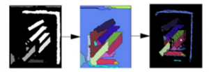
Figure 1: Watershed algorithm and colors assigning to Point cloud.

After objects are labeled, the data remains as unorganized objects data and will be segmented into each planar surface which represents for object cloud called cluster.

2.2.  3D image processing

When using 3D devices, the collected data often appears to be hovering and not in any plane. These points usually appear near the interface between surfaces, or near the edges of an object and. These points need eliminating, so the outlier filter is applied by considering the number of neighbor points K and the radius R of each point. If any point in point cloud whose number of neighbors in sphere of radius R is not greater than a threshold number, that point will be removed from point cloud. After that normal vector and the cluster segmentation are calculated. Normal vector is the most important point feature that distinguishes between different 3D cloud. the normal vector is the normative vector of a plane estimated from a given set of points. The problem of determining the normal to a point on the surface is approximated by the problem of estimating the normal of a plane tangent to the surface. To determine a plane equation in space, it is necessary to determine an x point in that plane and its normal vector  . The point x is determined by focusing on nearby points.

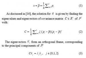
If the eigenvector  corresponding to the smallest eigenvalue . Therefore the approximation of  is  or . The calculation of the normal vector at the center will have errors, so to increase the reliability for the estimated vector, the maximum allowed error between the normal vector at the center and the normal vector at the adjacent point satisfy the following conditions:

Through conducting experiment, the = 5 ° is found to be appropriate.

Although the Kinect was placed perpendicular to the bin, the barrel edge point cloud still existed and connected to the real object in the bin formed an unexpected object in bin. When calculating the normal vector, the program will consider the barrel edge and the object are one object then the normal vector calculation and the position of the real object are not correct. Therefore, based on the normal vector, it is possible to separate the sides of the barrel with the idea that the angle between the two normal vectors on the side and the bottom edge will be larger than threshold value α. From experiment, the angle α = 50⁰ is appropriate. The results are shown in Figures 2 and 3.

The Euclidean clustering algorithm basically used to segment cluster and based on their neighbors [17]. Therefore, to estimate the normal vector to recognize that they belong to one plane, the Clustering procedure are through the following steps:

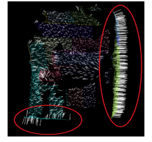
Figure 2: Normal vector of points

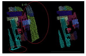
Figure 3: Image before and after removing barrel edge.

• Normal calculation of point cloud.
• Apply Kd-tree algorithm by define radius searching to find nearby points.
• Create list of cluster C and list of points to handle L.
• For every point in P, do the following step:
• Add in to L
• Search the list of neighbor n of within a sphere of radius r using kd-tree algorithm.
• For every neighbor , check if point exists in L. If it exists we skip to the next neighbor, otherwise we apply the following check.
• Calculate the angle between 2 point and its neighbor

• Determine the color difference of 3 channels R, G, B of 2 points:

• if the point  and its neighbor satisfies (5) and (6) then add to L, otherwise skip to the next neighbor.
• After checking all the points in L, put L into C and reset L.
• If the number of points in the cluster are in the range (Min_clust, Max_clust), it will save the cluster. Among the cluster that meet the conditions of color, normal, size, the cluster will be selected if it has the highest height as shown in Figure 4.

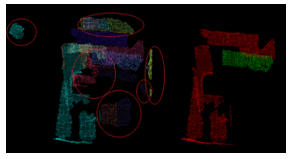
Figure 4: Image before and after extract cluster.

In Figure 4, the area circled to the left is the cluster having a smaller number of points than the Min_clust. Therefore, they were removed. Finally, the result is shown on the right with the green cluster which has the highest height. The robot will use this cluster to calculate the position and direction.

3. Manipulator and camera calibration

Because it is hard to determine the position of the camera coordinate that corresponds to the coordinate of the manipulator; therefore, using the method of measuring the distance from the manipulator to the camera will not give accurate results. Therefore, this research uses intermediate positions with known coordinates in both camera coordinates and manipulator to find transfer matrices. Suppose we have any point M in 3D real space, the coordinates of this point M in the camera coordinate system is denoted  and in the robot coordinate system is , then we have the formula to transfer coordinates from the camera coordinate system to the robot coordinate system as follows:

Where R is a rotation matrix and T is the translation matrix containing the translational vector from the robot origin to camera origin. If and  then (7) becomes:

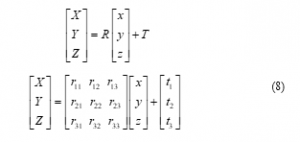
From (8), there are 12 variables to find, so it is necessary to have 12 equations corresponding to 12 variables, each point coordinates can only provide 3 equations so we need to take 4 points to be able to find two matrices R and T. After getting the necessary points, the system is solved as linear equation

With Kinect cameras, both 2D and depth images have a resolution of 640×480 and each pixel in 2D images corresponds to a point obtained from the depth camera. Kinect’s true coordinate system is defined to coincide with the color camera’s coordinate system, so when the pixel coordinates of a point in an RGB image are obtained, the x, y, and z values ​​of that point can be retrieved in the camera coordinates. So, the method to get coordinates is as follows: Use the Hough Circle algorithm to determine the center of a circle. From the pixel coordinates of the center of the circle in the color image, the center of the circle  in the camera coordinate system is retrieved as shown in Figure 5a. Then, use the Teach-pendant to control the manipulator’s head to the center of the circle to get the coordinates of this point in the robotic coordinate system. The work head needs to be small enough to increase accuracy Figure 5b. The data table of this process and error checking are shown in Table 1 and Table 2

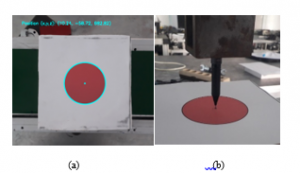
Figure 5: (a) Coordinate from camera, (b) coordinate from robot

Table 1: Coordinates from camera and robot

Point	Camera Coordinate (mm)	Robot Coordinate (mm)
1	-11.238; -95.1482; 798	298.218; -339.686; 0.0484
2	64.4799; -101.508; 680	289.673;-419.271; 120.996
3	-35.7193; -88.948; 746	307.759 -314.414 50.322
4	22.9576; 28.523; 741	427.611; -374.943; 51.3479

Table 2: Calibration error checking table

Camera coordinate (mm)	Robot coordinate (mm)	Absolute error (mm)
		X	Y	Z
48.2097; 15.5754; 790	414.531; -399.18; 1.72738	0.08498	1.2113	1.3723
-5.20496; 33.4604; 792	432.75; -344.522; 1.66852	0.7737	0.7121	2.4602
-29.8731; -62.924; 677	330.144; -319.86; 119.984	1.9182	2.0250	0.3202
14.6488; -16.0439; 743	378.403;-367.813; 51.472	2.4365	1.1975	0.2991
Mean error (mm)		1.3033	1.2865	1.1130

After identifying separated object, object is grasped and placed on the V-groove and there are eight case of placing as shown in Figure 6a. Since it is placed on a notched groove, the position of the object just changes along the axis of the groove. To determine the position O for grasping, it is only necessary to determine the coordinates of one point called the key point on the object as shown in Figure 6b and then using the dimension of the object to calculate the O position.

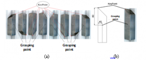
Figure 6: (a) eight cases placing on V-groove, (b) Key point and grasping point.

To determine the key point, Firstly, the template matching algorithm are performed then the Hough Line detection applied to find the line equation. Then based on line equation, the intersection point coordinate of each two lines are calculated. By combining each case result of template matching and calculated points, the appropriate coordinate of the key point is determined.

4. Experiment

Working space for experiment includes one RGB-D camera fixed above the working space, a monocular camera 2D attached at the end effector of Manipulator, the 6DOF Nachi Manipulator and pneumatic suction cup with maximum 1 kg payload and the V-groove for fine tuning location of object as shown in Figure 7. The 3D Camera is the Microsoft Kinect v1 with a resolution 640×480 combined with 2D camera Logitech. Both of them are parallel fixed with table surface having rectangular box objects. The specification of computer is: Laptop, RAM 16GB, Core I7, CPU 3.1GHZ. Six objects, representing for six random cases, are aluminium type and randomly stacked inside the box. They will be picked up and put at registered position.

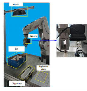
Figure 7: Experiment apparatus

By using 2D and 3D image processing discussed above, the positions of the objects are calculated as shown in Fig.8. The cluster having the highest height, green colour, is chosen to be grasped

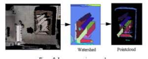
Figure 8: Image processing procedure

After having the coordinates and directions of object in the bin, the manipulator will perform the grasping task and then place it on the V-groove for the fine-tuning step Figure 9. After placing the object in the V-groove, the robot will use the second monocular camera to take the image to find the location and side of object to be picked Figure 10. Then the robot will put it to the registered position as shown in Figure 11.

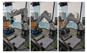
Figure 9: Process of grasping the object in the bin and putting it on V-groove

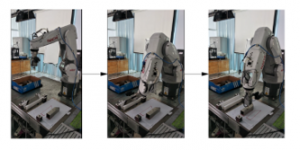
Figure 10: Process of grasping object on V-groove and putting it at registered

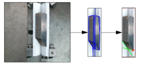
Figure. 11: Finding the key point of the object

After finish grasping task, the angular error, position error of the objects and the desired position are compared as shown in Figure 12. The real position of objects is obtained by reading the coordinate value on teach-pendant when moving robot manually. From that position the error of angle and position are calculated. The data are taken many times to calculate the mean error of the system as shown in following Table 3. The processing time is also calculated Figure 13

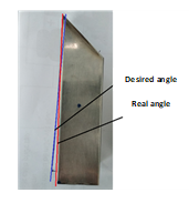
Figure 12: Desired position and real position

Table 3: Error position and angle calculation

No	Position Error (mm)			Angle error (degree)
	X	Y	Z
1	1.00	1.73	0.08	1.1243
2	1.25	1.62	0.11	1.6973
3	1.01	1.52	0.19	1.0981
4	1.18	1.91	0.36	1.8352
5	0.50	1.15	0.34	1.9559
6	1.61	1.27	0.52	1.0600
Mean Error	1.0917	1.533	0.2667	1.4618

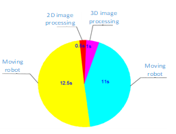
Figure 13: Processing time of system

From Table 3 it can be seen that the error of angle and position compared to the desired position is small and acceptable. The time to move the robot takes up most of the time by 23 seconds. Time to process images and data transmission is small about 1.5 seconds. The total time of implementation is 25 seconds, which is less than 30s. The image processing time is just about 6% of total time. To improve speed of system, the speed of robot could be increased to 100%. But for safety reasons it should only be done at 50% speed.

5. Conclusion

The paper proposed an effective method for the bin-picking problem. The image processing time is small and the accuracy is high. The method consists of two steps: the first step is to use the 3D camera and to combine 2D and 3D image processing for object segmentation and the second step is to use 2D camera for fining the grasping task. The effectiveness of the proposed approach was confirmed by a series of experimental results. The proposed method is also easy for installation and maintenance and applicable for assembly task in real industry. The comparing performance of proposed system and existing ones which are discussed in the introduction section are summarized in below Table 4.

Table 4: Comparing performance of Systems

	Proposed System	Existing system
Complexity	Not complicated	Very complicated
Time executing	Fast	Time consuming
Quality	Good and stable	Good and stable
Quantity	Mass product	Mass product
Setup	Easy	Complicated

Conflict of Interest

The authors declare no conflict of interest.

Acknowledgment

This research was supported by Saigon Hi-Tech Park Training Center and Vietnam National University, HoChiMinh City

1. F. Casado, Y.L. Lapido, D.P. Losada, A.S. Alonso, “ Pose estimation and object tracking using 2D image,” In 27th International Conference on Flexible Automation and Intelligent Manufacturing, Modena, Italia, 63-71, 27-30 June, 2017, doi: 10.1016/j.promfg.2017.07.134.
2. I. Wesis, M. Ray, “”Model-based recognition of 3D objects from single images,” IEEE Transactions on Pattern Analysis and Machine Intelligence, 23(2), 116-128, 2001, doi: 10.1109/34.908963.
3. K. Ban, F. Warashina, I. Kanno, H. Kumiya, ” Industrial intelligent robot,” FANUC Tech. Rev., 16(2), 29-34, 2003.
4. J. Xu, “ Rapid 3D surface profile measurement of industrial parts using two-level structured light patterns,” Optics and Lasers in Engineering, 49(7), 907-914, 2011, doi: 10.1016/j.optlaseng.2011.02.010.
5. W.C. Chang, C.H. Wu, “ Eye-in-hand vision-based robotic bin-picking with active laser project,” International Journal of Advanced Manufacturing Technology, 85, 2873–2885, 2016, doi: 10.1007/s00170-015-8120-0
6. K. Rahardja, A. Kosaka, “Vision-based binpicking: recognition and localization of multiple complex objects using simple visual cues,” In Proceedings of IEEE/RSJ International Conference on Intelligent Robots and Systems, 100-107, 1996, doi: 10.1109/IROS.1996.569005.
7. M. Berger, G. Bachler, S. Scherer, “ Vision guided bin picking and mounting in a flexible assembly cell,” In Proeeding of the 13th International Conference on Industrial & Engineering Applications of Artificial Intelligence and Expert Systems, 109-118, 2000, doi: doi.org/10.1007/3-540-45049-1_14
8. M.Y. Liu, O. Tuzel, A. Veeraraghavan, Y. Taguchi, T.K. Marks, R. Chellappa, “Fast object localization and pose estimation in heavy clutter for robotic bin picking,” The International Journal of Robotics Research, 31(8), 951–973, 2012, doi: 10.1177/0278364911436018
9. A. Adan, S.V. Andrés, P. Merchán, R. Heradio, “Direction Kernels: Using a simplified 3D model representation for grasping,” Machine Vision and Applications, 24(1), 351-370. 2013, doi: 10.1007/s00138-011-0351-y
10. R. D. Schraft, T. Ledermann, “Intelligent picking of chaotically stored objects,” Assembly Automation, 23(1), 38-42, 2003, doi: 10.1108/01445150310460079
11. K. Bousmalis, A. Irpan, P. Wohlhart, Y. Bai, M. Kelcey, M. Kalakrishnan, L. Downs, J. Ibarz, P. Pastor, K. Konolige, S. Levine, V. Vanhoucke, “Using simulation and domain adaptation to improve efficiency of deep robotic grasping,” In Proceedings of IEEE International Conference on Robotics and Automation (ICRA), 4243 – 4250, 2018, Australia, doi: 10.1109/ICRA.2018.8460875.
12. J. Mahler, J. Liang, S. Niyaz, M. Laskey, R. Doan, X. Liu, J.A. Ojea, K. Goldberg,” Dex-net 2.0: deep learning to plan robust grasps with synthetic point clouds and analytic grasp metrics,” In Robotics: Science and Systems, 245-251, 2017, doi: 10.15607/RSS.2017.XIII.058
13. L. Tuan-Tang, L. and Chyi-Yeu, “Bin-Picking for Planar Objects Based on a Deep Learning Network: A Case Study of USB Packs,” Sensors, 19(16), pp. 3602-3618, 2019, doi: 10.3390/s19163602
14. J. Chen, T. Fujinami, E. Li, “Deep Bin Picking with Reinforcement Learning,” In Proceedings of the 35th International Conference on Machine Learning, 1-8, 2018, Sweden.
15. S. K. Anton, V.S. Ilia, “An Overview of Watershed Algorithm Implementations in Open Source Librarie,” Journal of Imaging, 4(10), 123-138, 2018 doi: 10.3390/jimaging4100123.
16. L.D. Hanh, L.M. Duc, “Planar Object Recognition For Bin Picking Application,” In Proceedings of 5th NAFOSTED Conference on Information and Computer Science (NICS), 213-218, 2018, doi: 10.1109/NICS.2018.8606884.
17. Conditional Euclidean Clustering. Available online: http://pointclouds.org/documentation/tutorials/conditional_euclidean_clustering.php(accessed on 12 January 2020).

(Click Here)

(Click Here)