


Introduction
On 7 October 1994, a glacial lake outburst flood (GLOF) broke through the southern lateral moraine of Lugge glacial lake in the Lunana region of Bhutan (Fig. 1; 28°5.5′ N, 90°17.5′ E). The flood damaged local government facilities at Punakha and killed more than 20 people. Reference BhargavaBhargava (1995) estimated the flood volume as 23 × 106 m3, by analyzing hydrograph data at a site 242 km downstream from the lake. The Geological Survey of India in collaboration with the Geological Survey of Bhutan undertook a field investigation immediately after the event (Reference TashiTashi, 1994). They found a 23 m lowering of the lake level and estimated the flood volume to be 18 × 106 m3 based on the dimensions of the lake. Reference Leber, Häusler, Brauner and WangdaLeber and others (2002) recalculated the flood volume to be 18.7 × 10⁶ m3 from further hydrograph data. On the other hand, Reference Richardson and ReynoldsRichardson and Reynolds (2000) reported 48 × 106 m3 as the discharge volume without citing references or detailing methodology. We have found conflicting estimations such as those above in much of the literature concerning the GLOF of Lugge in 1994.
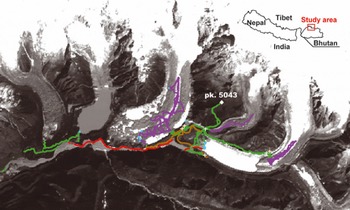
Fig. 1. Glaciers and glacial lakes in the Lunana region with gridcells of ground survey in 2004. Dots colored with red, purple, blue, brown and green denote topographically classified gridcells as riverbeds, glaciers, lakes, moraine ridges and hill slopes, respectively. White crosses are benchmarks for the ground survey. White rhombus is peak 5043 m a.s.l., the altitudinal reference point.
Many investigations of GLOFs have been carried out in this region (e.g. Reference Sharma, Ghosh and NorbuSharma and others, 1987; Reference AgetaAgeta and others, 2000; Reference HaeuslerHaeusler and others, 2000; Reference Iwata, Ageta, Naito, Sakai, Narama and KarmaIwata and others, 2002; Reference Leber, Häusler, Brauner and WangdaLeber and others, 2002), including mapping of glacial lakes in the Nepal and Bhutan Himalaya with satellite images (Reference Mool, Wangda, Bajracharya, Kuzang, Gurung and JoshiMool and others, 2001a, b). Although a topographical assessment is required to predict GLOF hazards (Reference Huggel, Kääb, Haeberli, Teysseire and PaulHuggel and others, 2002), no suitably precise map of the Himalaya is so far available. A promising remedy for this may lie in remote-sensing digital elevation models (DEMs) such as those available from the Advanced Spaceborne Thermal Emission and Reflection Radiometer (ASTER) on Terra or the Shuttle Radar Topography Mission (SRTM). Reference KääbKääb and others (2005) and Reference Quincey, Lucas, Richardson, Glasser, Hambrey and ReynoldsQuincey and others (2005) presented perspective overviews on the utilization of remote-sensing techniques for cryosphere-related hazards. Many attempts have been made to evaluate the accuracy of the ASTER DEM and SRTM DEM in mountainous regions (e.g. Reference Hirano, Welch and LangHirano and others, 2003; Reference Falorni, Teles, Vivoni, Bras and AmaratungaFalorni and others, 2005; Reference Fujisada, Bailey, Kelly, Hara and AbramsFujisada and others, 2005; Reference Berthier, Arnaud, Vincent and RémyBerthier and others, 2006; Reference Carabajal and HardingCarabajal and Harding, 2006). In the Bhutan Himalaya, Reference KääbKääb (2005) evaluated the reproducibility of ASTER DEMs compared with a merged SRTM and ASTER DEM. To date, however, these DEMs have not been validated with any ground-survey and/or aerophotogrammetric data in the high Himalaya because of a scarcity of observations and a lack of accurate maps. We attempt to re-evaluate the volume of the Lugge glacial lake GLOF and to evaluate the volumes of possible future GLOFs using the ASTER DEM and SRTM DEM, verified with the ground survey data in the Lunana region. In addition, we point out some possible outburst points of lakes in this region by showing the distance, altitudinal difference and gradient between the lake and the neighboring riverbed or other glacial lake.
Data Used
Ground survey by differential GPS
Surveys by a carrier-phase differential global positioning system (DGPS; CMC All Star receivers) and a digital theodolite with a laser distance meter (SET2100, SOKKIA Co., Ltd) were carried out on and around the glaciers and glacial lakes in Lunana in October 2004. The surveyed area (Fig. 1) is 10.7 km (east–west) by 3.4 km (north–south) and the altitude range is 927 m (4116–5043 m a.s.l.). Data post-processing of DGPS measurements was performed using Waypoint GrafNav/GrafNet software (NovAtel Inc.). The relative positions and altitudes of all points were calculated on a common Universal Transverse Mercator projection (zone 46N, WGS84 reference system) referenced to a peak 5043 ma.s.l. (white rhombus in Fig. 1), the location and altitude of which were adopted from a map published by the Survey of India in 1966. Relative measurement errors in the survey are evaluated by comparing the successive positions of 12 stable benchmarks that were installed around Lugge and Thorthormi glaciers and were measured more than once (white crosses in Fig. 1). Standard deviations of differences from the averages (29 measurements in total, two to three measurements for each benchmark) indicate measurement errors of 0.11 m horizontally and 0.17 m vertically. Data processed as unstable or that failed to converge to a solution (13%) were not included in subsequent analyses. The remainder of all surveyed points (194 783 points) were converted into gridcells by standard kriging methods, in which points utilized to obtain a gridcell altitude are limited to the circle with radius half of the diagonal of the targeted gridcell. Gridcells containing no measured points were excluded from the analysis. Resolutions of ground-survey gridcells were different from remote-sensing DEMs by as much as 15 × 15 m (4008 gridcells) for ASTER15 DEM, 90 × 90 m (487 gridcells) for ASTER90 DEM, and 3 × 3 arc-sec (506 gridcells) for SRTM DEM.
ASTER
A Level 3A01 product of ASTER ortho-images with a relative DEM product (spatial resolution of 15 m; ASTER15 DEM, hereafter) was used for this analysis. This is a semi-standard ortho-image generated from the Level-1A data by the ASTER Ground Data System (ASTER GDS) at the Earth Remote Sensing Data Analysis Center (ERSDAC) in Japan. The relative DEM is produced with the data of two telescopes, nadir-looking visible/near-infrared (VNIR) (band 3N) and backward-looking VNIR (band 3B) without ground-control point (GCP) correction for individual scenes. Stereoscopic images, the observational time difference of which is ∼55 s, taken over one region of the satellite’s flight direction, can be derived from these two separate datasets. The detailed algorithm for DEM generation is described by Reference Fujisada, Bailey, Kelly, Hara and AbramsFujisada and others (2005) or can be viewed at http://www.gds.aster.ersdac.or.jp/gds_www2002/exhibition_e/a_products_e/a_product2_e.html.
Reference ToutinToutin (2002) generated and validated ASTER DEMs in the Canadian Rocky Mountains using 10–20 GCPs. He showed root-mean-square errors (RMSEs) of 18–20 m in elevation by comparison with remaining independent checkpoints. Reference Hirano, Welch and LangHirano and others (2003) validated the ASTER DEM at four selected areas in Japan, the United States and the Andes Mountains. They showed an RMSE of altitudes in the Andes, a high-altitude and high-relief area of ±15.8 m by comparison with 53 map points. Reference Fujisada, Bailey, Kelly, Hara and AbramsFujisada and others (2005), whose algorithm was used for the DEM in this study, assessed the accuracy of the DEM with high-accuracy GCPs in Japan. The horizontal geolocation and altitudinal accuracy were 50 and ±10 m, respectively. They noted that the elevational differences were more pronounced in high-relief areas.
The image used in the analysis was obtained on 20 January 2001 in which no cloud or snow cover was found (Fig. 1). The location of the ASTER VNIR image was affine-transformed by referring to the boundaries of lakes and ponds, which were clearly seen in the image and were checked during the DGPS survey. The RMSE of the affine transformation was 5.99 m. The same transformation was adopted to the DEM. Another product, the spatial resolution of which is 90 m, was also used to evaluate the effect of different resolutions of gridcells (ASTER90 DEM, hereafter).
SRTM
The single-pass interferometric synthetic aperture radar (InSAR) SRTM mission in February 2000 provided a topography covering large sectors of the continents (60°N to 54°S; Reference Rabus, Eineder, Roth and BamlerRabus and others, 2003). The SRTM DEM with 3 arcsec spatial resolution is available for regions worldwide. Reference RodriguezRodriguez and others (2005) summarized the fundamental sources of errors in the SRTM DEM. Reference Carabajal and HardingCarabajal and Harding (2006) revealed that the standard deviations were >30 m for the rugged relief of Central Asia by comparison with the Ice, Cloud and land Elevation Satellite (ICESat). Only a few studies have reported the performance of SRTM in a glacial environment. Reference KääbKääb (2005) calculated the standard deviation of the height difference between an SRTM DEM and an aerophotogrammetric DEM as ±20 m for the Swiss Alps and as ±15 m for southern Patagonia. Reference Berthier, Arnaud, Vincent and RémyBerthier and others (2006) found significant altitudinal biases (7 m every 1000 m) with a standard deviation of height difference of ±22 m for the French Alps. The SRTM DEM (version 1) for the Lunana region (28° N, 90° E) can be downloaded at ftp://e0srp01u.ecs.nasa.gov/srtm/version1/Eurasia/
Comparison of Different Topographic Datasets
Accuracy evaluation
We first compare the three DEMs (ASTER15, SRTM and ASTER90) with the DGPS ground survey DEM (Fig. 2). Because no GCP is available in the region and the absolute accuracy of old maps is uncertain, the DGPS altitudes are not absolute, but relative. Therefore, the altitudinal shifts (dZ) shown in Figure 2 are not of concern since our purpose is the assessment of local (rather than large-scale) topography. The standard deviations (i.e. the RMSE) of the height differences, however, are important. They show better relative accuracies than those in previous studies. Our analysis shows a significant lowering of the largest altitudes (approximately 5000 m a.s.l.) in both ASTER15 and SRTM DEMs (Fig. 3) as Reference Berthier, Arnaud, Vincent and RémyBerthier and others (2006) pointed out. It is unclear, however, whether the reasons for this are the same as found by Reference Berthier, Arnaud, Vincent and RémyBerthier and others (2006) or whether it is due to an insufficient number of gridcells sampled for comparison. On the other hand, the terrain slope between the gridcells affects the RMSE (Fig. 4), while no bias is found in any DEMs except in the case of the largest slope (>40°). Reference ToutinToutin (2002) mentioned that the RMSEs of the ASTER DEM were almost linearly correlated with the terrain slope. The increase in the RMSE with terrain slope is clear in the SRTM DEM and ASTER90 DEM, and more than in the ASTER15 DEM. The influence of terrain slope is more obvious in the resolution SRTM and ASTER90 because the area of the SRTM gridcell is roughly 35 times larger than that of ASTER15.
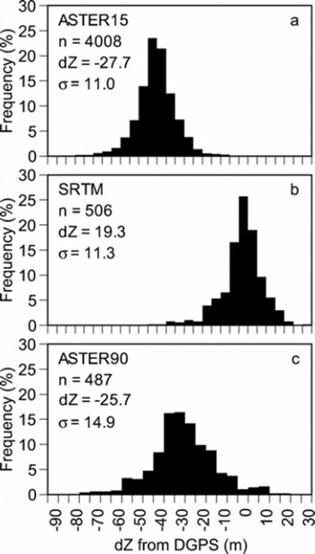
Fig. 2. Histograms of altitudinal differences with 5 m interval of (a) ASTER15 DEM, (b) SRTM DEM and (c) ASTER90 DEM.
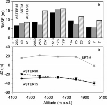
Fig. 3. (a) Altitudinal biases and (b) RMSEs for ASTER15 DEM, SRTM DEM and ASTER90 DEM versus altitudes. Altitudes are from DGPS DEM. Numbers of gridcells are shown between panels. Error bars in (b) denote standard errors.
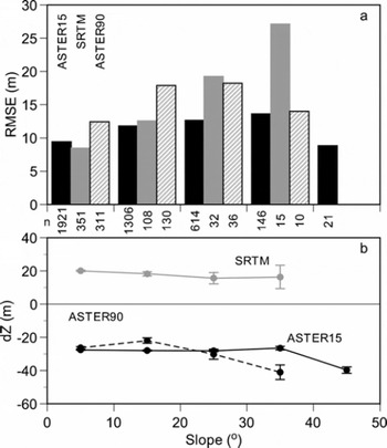
Fig. 4. (a) Altitudinal biases and (b) RMSEs for ASTER15 DEM, SRTM DEM and ASTER90 DEM versus terrain slopes. Terrain slopes are of each remote-sensing DEM. Numbers of gridcells are shown between panels. Error bars in (b) denote standard errors.
If the measurement density in a gridcell is small and/or the surveyed points are located at a corner of a gridcell, the generated altitude of the gridcell in the DGPS DEM is less reliable. In order to evaluate the influence of DGPS DEM quality, we generated an alternative small grid with one-tenth of the resolution of the original grid (called ‘small-cell’; elevational information not included), in which no cell without measurement point is included. Thus small-cells with resolutions of 1.5 m, 9.0 m and 0.3 arcsec are generated for the ASTER15, ASTER90 and SRTM DEMs, respectively. Figure 5 shows the altitudinal bias and RMSE compared with the small-cell measurement density in each gridcell. If a gridcell is measured completely by DGPS, the density will be 100%. For all DEMs the altitudinal bias shows no obvious dependence on the measurement density. The RMSE shows no significant trend with measurement density in the ASTER15 DEM, whereas the increase of measurement density gives significantly (F-test for variances at 95% level) lower RMSEs in the SRTM and ASTER90 DEMs. If the SRTM DEM gridcell has more than a 10% measurement density, the relative accuracy of the DEM may reach a sufficient level (resolution smaller than total averages). No significant correlation is found between measurement density and terrain slope. The altitudinal bias and RMSE are also compared with normalized distance between the center of the gridcell and the averaged center of small-cells included in the gridcell (Fig. 6). Normalized distance is obtained by dividing the distance between the two centers by half of the diagonal of the gridcell. No significant dependences are found in the ASTER15 DEM because the resolution of the gridcell may be sufficiently small. With the SRTM and ASTER90 DEMs, however, the relative DEM accuracies are compromised when the normalized distance increases more than 0.8. Because the elevation of an SRTM3 (3 arcsec) cell is an arithmetic average of nine original SRTM1 cells (1 × 1 arcsec), the large RMSE with large normalized distance is derived with less reliable horizontal accuracy in the DGPS DEM. In other words, we possibly compare cells in different locations if the normalized distance approaches one. Although the RMSE in the DEM evaluation may be attributed to both the remote-sensing DEMs and the ground-survey DEM, it is sufficiently small to use for the assessment topography around the glacial lakes in the target region. In all cases, the ASTER90 DEM shows larger relative errors, due to the larger resolution of the gridcell.
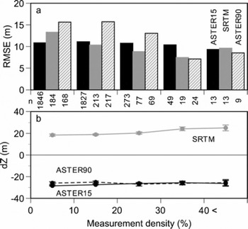
Fig. 5. (a) Altitudinal biases and (b) RMSEs for ASTER15 DEM, SRTM DEM and ASTER90 DEM versus measurement density (%) in each gridcell. Numbers of gridcells are shown between panels. Error bars in (b) denote standard errors.
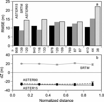
Fig. 6. (a) Altitudinal biases and (b) RMSEs for ASTER15 DEM, SRTM DEM and ASTER90 DEM versus normalized distance between grid center and averaged center of small-cells. Numbers of gridcells are shown between panels. Error bars in (b) denote standard errors.
Assessment of errors for various topographic features
The development of moraine-dammed glacial lakes results from glacier retreat and downwasting particularly of debris-covered glaciers (e.g. Reference YamadaYamada, 1998; Reference Richardson and ReynoldsRichardson and Reynolds, 2000; Reference Benn, Wiseman and HandsBenn and others, 2001; Reference Quincey, Lucas, Richardson, Glasser, Hambrey and ReynoldsQuincey and others, 2005, Reference Quincey2007). Outbursts from moraine-dammed lakes occur mainly through the degradation of buried ice within the dam, by seepage and piping through the dam, or by overflowing and erosion by waves from avalanches entering the lake (Reference Clague and EvansClague and Evans, 2000; Reference Richardson and ReynoldsRichardson and Reynolds, 2000). Although it is difficult to predict ‘when’ a GLOF occurs since an outburst is a fracture event, it is possible and also important to focus on ‘where’ it will occur (e.g. Reference Richardson and ReynoldsRichardson and Reynolds, 2000). We need, therefore, to study the topography around a glacial lake when assessing the potential for a GLOF (Fig. 7).
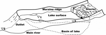
Fig. 7. Schematic figure of the structure of a glacial lake. Triangles denote elevations at lake surface (1), where the outlet channel meets the main river (2) and where the main riverbed is at the lake surface (3).
We classify the gridcells into five topographical categories (ponds/glacial lakes, glaciers, riverbeds, moraine ridges, and other hill slopes) based on the ground survey in 2004 (Fig. 1). Figure 8 shows for each DEM, the RMSE, the altitudinal difference from the average, and the average slope angle of each topography. The RMSEs are lower over lakes/ponds, river beds and glacier surfaces, yet higher over moraine ridges and hill slopes, compared with non-categorized RMSEs. In particular, the altitudinal biases in moraine ridges were clearly lower in all DEMs because the grid height of the ground survey represents the top of the ridge, whereas the height of the remote-sensing DEMs is dragged down by the surrounding lower hill slopes. Topographic categorization is another aspect of categorization by terrain slope (Fig. 8c). Lake, glacier and riverbed surfaces have lower slopes, with smaller RMSEs than moraine ridges and hill slopes with large RMSEs for ASTER15. We found significant correlations between RMSE and slope for ASTER15 and SRTM (p < 0.05). Higher terrain slopes for ASTER15 than SRTM and ASTER90 are probably due to gridscales.
Although the DEM altitudes of lakes and ponds seem to exhibit good relative accuracy, Reference ToutinToutin (2002) pointed out a large uncertainty in the altitude of water surfaces indicated by the ASTER15 DEM, because of the lack of clear features with which to generate the DEM. We also find a large variability of grid height on lakes/ponds in both Raphstreng and Lugge glacial lakes. However, our validation suggests the ASTER15 DEM (and the SRTM DEM) works well at the edge of the lakes because the boundaries of water bodies and surrounding debris provide an obvious contrast for DEM generation. In addition, annual and seasonal changes in lake levels produce altitudinal biases and increase RMSE in the lake level. Few studies have been reported concerning changes in glacial lake level, other than that of Reference YamadaYamada (1998) in which the water level of Tsho Rolpa glacial lake in the Nepal Himalaya fluctuated periodically within 2 m (highest in summer, lowest in winter) during observation over 3 years. Changes in the lakefront of Lugge glacial lake between 1994 and 2001 support negligible change in the lake level after the GLOF in 1994 (see details in the next section).
A number of studies have derived volume changes in glaciers using remote-sensing DEMs and topographic maps (e.g. Reference Muskett, Lingle, Tangborn and RabusMuskett and others, 2003; Reference Rignot, Rivera and CasassaRignot and others, 2003; Reference Sauber, Molnia, Carabajal, Luthcke and MuskettSauber and others, 2005; Reference Surazakov and AizenSurazakov and Aizen, 2006), but the SRTM DEM may have significant altitudinal and/or regional biases (Reference Berthier, Arnaud, Vincent and RémyBerthier and others, 2006; Reference Surazakov and AizenSurazakov and Aizen, 2006). In the Lunana region, we have found that glacier surfaces have lowered by 3–5 m a−1 since 2002. Altitudinal biases of the glacier surface should be larger than for a riverbed, because the glacier surface in the DGPS DEM survey in 2004 is expected to be lower than those in the DEMs of 2000 (SRTM) and 2001 (ASTER). However, the difference in altitudinal bias between a glacier and a riverbed is negligible compared with the RMSE (Fig. 8). Although a longer time is necessary to detect altitudinal change of a glacier surface from remote-sensing DEMs, Figure 8 suggests that the altitude of riverbeds or rather flat areas, which are expected to be unchanged, may provide good references for altitude. This analysis implies that we can use remote-sensing DEMs more accurately if we classify the topographical features carefully.
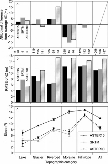
Fig. 8. (a) Altitudinal differences from averaged altitudinal biases, (b) RMSEs and (c) terrain slopes for ASTER15 DEM, SRTM DEM and ASTER90 DEM categorized by topographic features such as lake, glacier, riverbed, moraine and hill slope. Numbers of gridcells are shown between panels. Error bars in (c) denote standard errors.
Analysis of Glacial Lakes
GLOF of 1994 revisited
We first attempt to re-evaluate the volume of GLOF from Lugge glacial lake in 1994. Reference TashiTashi (1994) reported a 23 m lowering of the lake level, whereas Reference Iwata, Ageta, Naito, Sakai, Narama and KarmaIwata and others (2002) indicated a 10 m lowering. Both levels were estimated by visual inspections. We evaluate the change in height by DGPS measurement in situ and the change in extent of the lake before/after the GLOF by satellite images. Figure 9 shows satellite images around Lugge glacial lake taken in December 1993 (SPOT-XS; before the GLOF), in December 1994 (SPOT-3; after the GLOF) and in January 2001 (ASTER for the DEM). The images in 1993 and 1994 are transformed to the scene of 2001 by selecting eight reference points around the lake (Fig. 9).
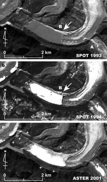
Fig. 9. Images around Lugge glacial lake taken in (a) December 1993 by SPOT-XS, (b) December 1994 by SPOT-3 and (c) January 2001 by ASTER. Crosses in (c) denote reference points to transform other images taken by SPOT in 1993 and 1994 into this image. Possible triggers of GLOF in 1994 are suggested by Reference Leber, Häusler, Brauner and WangdaLeber and others (2002) (A) and this study (B with arrow).
In orderto evaluate the changes in lake level and lakefront through the GLOF, the contour map around the end-moraine is drawn from the ASTER15 DEM (Fig. 10). Artificial contour lines on the lake surface, which are produced by the unclear features of the water surface (Reference ToutinToutin, 2002), are eliminated. The lakefront has lowered during the GLOF event, while it seems to have been stable between 1994 and 2001, with small changes only in lake levels. We obtained altitudes of water levels in 1993 and 2004 as 4496.9 ± 0.1 m a.s.l. (86 points) and 4513.8 ± 3.0 m a.s.l. (140 points), respectively, using DGPS point data (crosses in Fig. 10). The lakefront in 2004 was clear, and thus the measurement error is small. The lakefront in 1993, on the other hand, was identified during the measurements in situ by referring to the vegetation boundary and other surface morphology. The lowering of the lake level is calculated as 16.9 ± 3.2 m. Areas of the lake obtained from Système Probatoire pour l’Observation de la Terre (SPOT) images were 1.14 km2 in December 1993 and 0.90 km2 in December 1994. We re-evaluated the GLOF volume as (17.2 ± 5.3) × 106 m3 using the average area (1.02 ± 0.12 km2). Our re-evaluation is closer to the estimates of Reference TashiTashi (1994), Reference BhargavaBhargava (1995) and Reference Leber, Häusler, Brauner and WangdaLeber and others (2002), rather than to Reference Richardson and ReynoldsRichardson and Reynolds (2000). We believe our volume estimation of (17.2 ± 5.3) × 106 m3 is more reliable than previous estimates because ours is based on a combination of observations in situ (height change) and remote-sensing data (areal change).
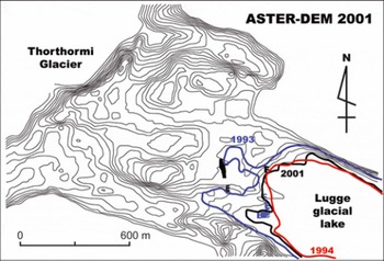
Fig. 10. Contour maps around end-moraine of Lugge glacial lake generated with ASTER15 DEM. Thick lines denote lakefront traced from images in 1993 (blue), 1994 (red) and 2001 (black). Crosses denote DGPS measurement points of lakefront in 1993 (black crosses) and 2001 (blue crosses).
Reference Leber, Häusler, Brauner and WangdaLeber and others (2002) suggested that an outburst from an upper pond triggered the GLOF in 1994 (A in Fig. 9). However, no obvious change in surface features of Lugge glacier was found between the SPOT images in 1993 and 1994. We propose here an alternative cause of the GLOF. The arrow in 1994 (B in Fig. 9b) shows the vestige of a collapse of the right bank of moraine. Although the spatial resolution is coarse, this feature was not found in the image of 1993 (B in Fig. 9a). During the field observation in 2004, we were forced to make a detour to avoid this collapsed moraine. This collapse is a possible cause of the 1994 GLOF.
Elevation analysis of glacial lakes
Topographical categorization allows more precise assessment of the GLOF. We have focused upon the narrow sections of the moraine ridge. However, the lower section of riverbed compared with the lake level, for which a precise DEM is required, is more important (Fig. 7). We focus now on the altitudinal difference between lake level and the adjacent riverbed (Fig. 11b). The levels of three glacial lakes/ponds, the riverbed and the moraine ridge are plotted in the projected cross-section based on the DGPS DEM. The extents of the lakes/ponds are derived from the ASTER image taken in 2001. Pond levels of Thorthormi glacier, which were measured at four different ponds (Fig. 1), suggest that water channels within the glacier are connected. We can find only three sections in which the riverbed is lower than the lake level (Fig. 11b). Even if the main river is adjacent to a large pond with the narrow moraine on the south side of Thorthormi glacier (Fig. 1), it does not matter if the water level is lower than the riverbed (Figs 7 and 11b). Since the outlet is the most likely break point for a GLOF (Fig. 7), we extract the altitudinal differences and gradients between the lake outlet and juncture of the river and outlet channel (Fig. 11; Table 1). Although some altitudinal disagreements are found among the different DEMs, we note some of the more obvious features. There is a minor chance of a GLOF given the present situation at Lugge glacial lake (Table 1, case 1) since the water level is now about 10 m higher than the outlet juncture, and with low gradient, although the lake is expanding year by year. Both outlet junctures of Thorthormi and Raphstreng glacial lakes have significant altitudinal differences from the lakes themselves, with a moderate gradient of about 10% (Table 1, cases 2 and 3). On the other hand, a significant altitudinal difference with a quite large gradient is found between the adjacent two lakes, Thorthormi and Raphstreng (Table 1, case 4). Although the possibility of a GLOF through the moraine between the two lakes has been pointed out (Reference Richardson and ReynoldsRichardson and Reynolds, 2000), the altitudinal difference has not been measured precisely. Because the altitudinal differences and gradients before the GLOF of 1994 are, respectively, 30–34 m and 5–6%, all cases other than Lugge glacial lake show some potential for GLOF, which should not be ignored.
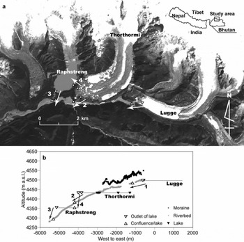
Fig. 11. (a) Possible section where GLOFs occur and (b) projected cross-section in west–east direction. Arrows with numbers denote possible sections of GLOF where the lake level is higher than the riverbed or neighboring lake. Gray lines denote extent of each glacial lake in the eastward direction. Altitudinal differences and gradients are summarized in Table 1.
Table 1. Altitudinal differences (m) and gradient (%) between lake level and juncture of river and outlet channel, area (km2) and maximum depth (m) of the glacial lakes in Lunana. Horizontal distances between outlet and juncture (between lakes for case 4) are obtained from the ASTER image taken in 2001 in order to calculate the gradients. Locations of each case are shown in Figure 11. Maximum depths of Lugge and Raphstreng glacial lakes are cited from Yamada and others (2001) and Reference BhargavaBhargava (1995), respectively

Volume estimation in case of GLOFs provides significant information for planning risk mitigation. Bathymetric profiles were measured for Raphstreng glacial lake (Reference BhargavaBhargava, 1995) and Lugge glacial lake (Reference YamadaYamada and others, 2004). However, it is practically impossible to measure the bathymetric profiles of ponds on Thorthormi glacier, because many ponds are now expanding and aggregating on the glacier. Table 1 shows that the glacial lakes of Lunana have high potential for a GLOF with a volume similar to that of 1994.
Conclusions
The potential for GLOFs in the Lunana region was assessed using DEMs generated from ground survey carrier-phase differential GPS, ASTER and SRTM. We evaluated the relative accuracy of elevations indicated by the ASTER DEM and SRTM DEM, by comparing with the ground-survey data. Topographical classification allows us to partition the total error in both DEMs into those in the terrain class. This classification enables better evaluation of altitudes of lakefronts, glacier surfaces and riverbeds, although it is less useful for moraine ridges and hill slopes because the terrain slope is significantly correlated with the topography. Using satellite images and the DEMs, we have re-evaluated the volumes and examined causes of the 1994 GLOF. In addition, we point out the sections where future GLOFs could occur, showing altitudinal differences and gradients around the glacial lakes.
One of the GLOF-triggering events is considered to be the melting of ice inside the moraine, which is damming water. Photogrammetric analysis of aerial photographs, which showed high accuracy, helped monitor the possible outburst trigger in the Swiss Alps (Reference Haeberli, Kääb, Vonder Mühll and TeysseireHaeberli and others, 2001). However, our study reveals that the remote-sensing DEMs from space are not applicable for monitoring altitudinal changes in a moraine ridge because of its inferior altitudinal relative accuracy. Monitoring at the site, therefore, is still crucial in addressing GLOF problems, even in this age of remote-sensing technology. GLOFs have been a serious problem in Himalayan countries. It is our hope that this study might not only present some sort of scientific advance, but also contribute to the daily lives of the local people who even now face the ongoing risk of GLOFs.
Acknowledgements
We thank the staff of the Geological Survey of Bhutan for the opportunity to conduct field research in the Lunana region. We are deeply obliged to the people who assisted us in the field. Special thanks are due to A.B. Surazakov and an anonymous reviewer for helpful comments. This analysis was supported by a Grant-in-Aid for Scientific Research (Project 19253001) from the Ministry of Education, Culture, Sports, Science and Technology of Japan.


