


Introduction
The atmospheric and oceanic conditions that govern the mass balance of the Greenland ice sheet (GrIS) are displaying a warming trend. Atmospheric temperatures, measured by coastal Greenlandic weather stations, have been increasing in recent decades, most notably along the west coast of Greenland (Reference BoxBox, 2002). Higher atmospheric temperatures contribute to higher surface melt rates of Greenland glaciers. Besides the direct effect of a reduction in ice mass through enhanced melt, the higher melt rates could trigger a speed-up of glacier flow through basal lubrication, accelerating the drainage of the ice sheet (Reference Rignot and KanagaratnamRignot and Kanagaratnam, 2006). Marine-terminating glaciers in particular, such as Jakobshavn Isbræ/Sermeq Kujatdleq (Reference Holland, Thomas, de Young, Ribergaard and LyberthHolland and others, 2008) and Helheimgletscher (Reference JoughinJoughin and others, 2008), have demonstrated high sensitivity to local climatic conditions. Since there is a >400 km long succession of small to large-sized calving glaciers in Melville Bay (northern Baffin Bay region; Fig. 1), the consequences for the local glaciers and the GrIS could be extensive in a changing climate.
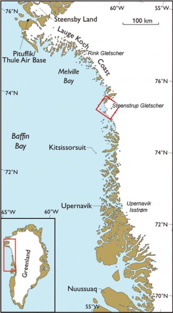
Fig. 1. Map of the Baffin Bay region of northwest Greenland. The boxed area at Steenstrup Gletscher outlines the coverage of Figure 2.
Signs of ice-mass change in northwest Greenland are already starting to show. Ice, Cloud and land Elevation Satellite (ICESat) observations suggest that the ice sheet in the coastal Melville Bay region experienced a drastic dynamic thinning of ∼0.5 m a−1 between 2003 and 2007, similar to the changes in the southeastern GrIS and the major calving outlet glaciers (Reference Pritchard, Arthern, Vaughan and EdwardsPritchard and others, 2009). Recently, Reference Khan, Wahr, Bevis, Velicogna and KendrickKhan and others (2010) pointed out an accelerated mass loss from northwest Greenland based on Gravity Recovery and Climate Experiment (GRACE) satellite data from 2003 to 2009. Possibly related to this is the regional retreat of glaciers draining into Melville Bay over the past few years to decades, such as observed at the large Rink Gletscher (76.2° N) and Steenstrup Gletscher (75.2° N) (Reference Dawes and van AsDawes and Van As, 2010); it is known from modelling studies that there can be a large dynamic response of marine-terminating glaciers to changes in frontal conditions (Reference Nick, Vieli, Howat and JoughinNick and others, 2009).
In this paper, we focus on the southern region of Melville Bay (Fig. 1), where the observed changes in surface height and frontal positions have been largest. Figure 2 shows the glacier front positions of Steenstrup and neighbouring glaciers, obtained from satellite imagery and aerial photography. Steenstrup Gletscher has retreated 10 km over the past 60 years, and ∼20 km over the past century judging from the first detailed mapping of the region by J.P. Koch in 1916. The front of Kjer Gletscher, until recently separated from Steenstrup Gletscher by Red Head peninsula, was fairly stable during most of the observation period. However, it has retreated since the northern part of the glacier lost the buttressing effect of Red Head in 2005. The cause of changes in calving glaciers in Greenland has been debated extensively over past years (e.g. Reference Joughin, Abdalati and FahnestockJoughin and others, 2004). The systematic retreat of glaciers along the entire coastline of Melville Bay cannot be explained by the natural variability displayed by calving glaciers, which are known to advance and retreat periodically in a steady climate (Reference ClarkeClarke, 1987), but must be a sign of past or present-day changes in climatic conditions. Causes should be sought amongst current or past changes in atmospheric temperature, sea-water temperature (Reference Holland, Thomas, de Young, Ribergaard and LyberthHolland and others, 2008) or precipitation (Reference BurgessBurgess and others, 2010).

Fig. 2. Modified Landsat image of Steenstrup Gletscher in 1999 showing glacier extent in 1916 (white), 1949 (red), 1963 (orange), 1975 (yellow), 1985 (green), 1999 (blue), 2007 (pink) and 2009 (purple). The white curve is taken from a hand-drawn map by L. Koch. Other curves are based on aerial and satellite imagery. The position of the AWS is marked with a star. See also Reference Dawes and van AsDawes and Van As (2010).
Automatic weather stations (AWS) are capable of monitoring the near-surface atmospheric conditions in remote and inaccessible places such as the Melville Bay region of the GrIS, and provide excellent tools to determine the energy exchange between the atmosphere and the glacier surface. Currently there are ∼30 permanent AWS on the GrIS, installed by the Cooperative Institute for Research in Environmental Sciences (CIRES; Reference Steffen, Box and AbdalatiSteffen and others, 1996), the Institute for Marine and Atmospheric Research Utrecht (IMAU) and the Geological Survey of Denmark and Greenland (GEUS; Reference AhlstrømAhlstrøm and others, 2008). Since no near-surface measurement records existed in the Melville Bay region of the GrIS, an AWS was placed on a slow-moving branch in the lower regions of Steenstrup Gletscher in 2004 (Fig. 2). In this paper, we aim to present the temperature changes in Melville Bay over the past decade and to provide a detailed surface energy budget for the AWS location on Steenstrup Gletscher. This is an exploratory and first in situ study in a region undergoing substantial glacial change. Observed climate data are used to quantify and put into a regional perspective the long-term temperature trends in the Melville Bay region using land-station data of the Danish Meteorological Institute (DMI). AWS data from Steenstrup Gletscher are used to present the local atmospheric conditions, and to give a detailed description of the local surface mass budget as derived from energy-balance modelling.
Methods
Observational records from land stations
This study uses data collected by weather stations both on land and ice. Land-station temperature data were purchased from the DMI. Continuous meteorological observations in the Melville Bay region were initiated in September 1981, on the island of Kitsissorsuit located 130 km south of Steenstrup Gletscher (Fig. 1). Longer time series are available from Pituffik/Thule Air Base (since 1974), Upernavik (since 1873) and Nuussuaq (since 1961), which are respectively 330 km northwest and 280 and 520 km south of Steenstrup Gletscher. Upernavik data are used, but are not the focus of this study; we chose to use Nuussuaq data for more pronounced zonal temperature gradients. Besides discussing the zonal temperature gradients, we also present measurements from Daneborg, located approximately at the same latitude as Kitsissorsuit (74° N), but on the east coast of Greenland. We calculated monthly means from the DMI data, provided that at least 50% of all monthly measurements were successful; otherwise the mean value cannot be considered representative of the full month. A second requirement was an equal spread of observation times capable of capturing the full daily cycle (i.e. not just daytime values). Rare occurrences of values outside the two-standard-deviation range of monthly means were considered erroneous and not taken into account. We focus on the period during which all four stations produced data simultaneously, i.e. since 1982 (data coverage from Kitsissorsuit in late 1981 did not meet the 50% data coverage criterion).
Other data were obtained from weather stations installed on the ice. Ablation data from the JAR (Jakobshavn ablation region) transect on the ice margin in the Ilulissat region (69.5°N) were provided by CIRES, who maintain the Greenland Climate Network (GC-Net; Reference Steffen, Box and AbdalatiSteffen and others, 1996). Finally, we also used data collected by an AWS positioned on Steenstrup Gletscher (Fig. 2).
The Steenstrup Gletscher AWS
The AWS on Steenstrup Gletscher was placed on a slow-moving and fairly flat ice patch next to the calving front and main ice stream on 28 April 2004. The position of the station (75°14.2′ N, 57°44.8′ W; 190 m a.s.l.) is such that no continuous data series have been obtained on the ice sheet within a 230 km radius, and within the ablation zone, over a much larger radius. Initially the station was installed as a basic ablation station, measuring ice ablation, temperature in the logger enclosure and relative humidity. On 18 July 2006 the station was upgraded to a full AWS. When the station was dismantled in September 2008, it was found with the battery and sensor cables torn out of the logger enclosure due to compacting snow in spring, providing us with a lower estimate of wintertime accumulation. The last recorded data originate from 10 April 2008.
The skeleton of the AWS consisted of an aluminium tripod with a lower and upper horizontal boom attached (Fig. 3). The frame of the station was not drilled into the ice, but was sinking with the ablating ice surface, allowing a fixed sensor height during the ice melt season. The AWS was equipped to measure air temperature, T, relative humidity, q R, wind speed, u, and direction, incoming (S in) and reflected (S rfl) shortwave radiation and incoming longwave radiation, L in, using the sensors listed in Table 1. The ice-height changes were monitored by pressure transducer (see below). Also station tilt and orientation were monitored by inclinometer and compass. Measurements were taken every full hour and data were stored locally in a Campbell CR10X data logger. In addition, data were transmitted four times per day during summer, when a solar panel provided a surplus of energy. Temperature, humidity and wind sensors were mounted on the upper boom at 2.5–3 m above the ice surface. The radiation instruments were mounted on the lower boom at ∼1.2 m height.

Fig. 3. Photograph from the measurement site on Steenstrup Gletscher taken after upgrading the ablation station to a full
Table 1. List of sensors and their accuracies as reported in the sensor manuals

The AWS was not equipped with a sonic ranger, but ice ablation (which is synonymous with net ablation/net balance in the ablation zone) was measured using a pressure transducer enclosed in a liquid-filled hose (50% ethylene glycol (antifreeze) solution) and steam-drilled into the ice (Reference Bøggild, Olesen, Ahlstrøm and JørgensenBøggild and others, 2004). Ablation can be deduced from the changes in the vertical liquid column as recorded by the transducer. An advantage of this system is that it can be left to measure for years on end, whereas a stake set-up with sonic rangers needs to be re-drilled regularly in melt regions. A disadvantage is that wintertime accumulation cannot be recorded. Capturing the mass of accumulation is a recurring problem in AWS studies as the density of snow and the change therein cannot be monitored.
Data treatment of the Steenstrup Gletscher AWS
The tilt correction of the incoming shortwave radiation record is essential, as this is the dominant parameter when it comes to ablation in Greenland (Reference Van de Wal, Greuell, van den Broeke, Reijmer and OerlemansVan de Wal and others, 2005). The type of sensor used in this study, the double-domed Kipp & Zonen CM7, is sensitive to beam direction (Reference Van den Broeke, van As, Reijmer and van de WalVan den Broeke and others, 2004), and will give inaccurate measurements in clear-sky conditions when tilted. S in is corrected using the fact that the radiation is composed of a diffuse and direct beam part, of which only the direct component requires adjustment. For a horizontal sensor, the direct beam component equals S in reduced by its diffuse fraction, f dif. For a tilted sensor, S in is determined from the measured value, S in,m, following
where C is the direct beam correction factor using a complex but straightforward algebraic transformation with sensor tilt values and direct-beam direction. From this we obtain
where f dif is estimated to range from 0.2 for clear skies to 1 for overcast conditions (Reference Harrison, Chalmers and HoganHarrison and others, 2008), assuming a linear dependency on the cloud fraction. Cloud fraction is approximated from the dependence of near-surface temperature on L in. The relationships between L in and near-surface T for both clear and cloudy conditions at each site (Reference Van As, van den Broeke, Reijmer and van de WalVan As and others, 2005) showed excellent agreement with the equation for clear-sky longwave dependency on T by Reference SwinbankSwinbank (1963), and black-body radiative dependency on T for overcast conditions. Linear interpolation between these clear and cloudy estimates produces an estimate of the cloud fraction for certain pairs of L in and T measurements. Values below and exceeding the range of theoretical incoming longwave radiation values were assumed to have been recorded in clear and overcast conditions respectively.
Due to a faulty sensor the relative humidity record was deemed unusable from July 2006 onward. This shortcoming required us to estimate humidity in order to be able to calculate the surface energy balance, which is possible due to the high dependency of specific humidity on temperature. Using the 2004–06 q R and T values we calculated mean q R values for every 1° temperature bin and fitted a polynomial to approximate q R from T for 2006–08. Even though the mean standard deviation of the temperature bins is relatively low (16%) due to the generally moist atmosphere at the AWS site (mean value 76%), we only present 30 day running-mean values of the surface energy balance. Doing so averages out inaccuracies due to the q R estimate on daily and synoptic timescales.
Surface energy-balance models calculate ablation rates that can be validated using surface height observations, but generally need accumulation observations to introduce a snow layer. However, there is no measured precipitation record available within a radius of hundreds of kilometres of the AWS. All we know from the radiation measurements, performed at 1.2 m above the ice surface, is that the lower boom of the station has not been covered by the snowpack between 2006 and 2008. It was necessary to introduce a modelled wintertime snow layer to be able to calculate the winter and spring energy fluxes (next subsection). Therefore we included an accumulation of 1 × 10⁻³ m w.e. during hours with subfreezing temperatures and a thick cloud cover. The occurrence of a thick cloud cover is identified from moments during which downwelling longwave radiation exceeded the black-body emission calculated using near-surface air temperature. The accumulation rate is tuned so that the modelled start of the ice-melt season corresponded to the observed start as shown from pressure transducer readings. Because it is tuned, the only potential inaccuracy due to a mismatch between modelled and actual snow thickness is in the calculation of the subsurface heat flux in winter, or during other short periods with a snow cover present. All other calculated surface energy fluxes will be unaffected by inaccuracies in snow thickness. This is shown in a sensitivity study in the Results section. Furthermore, we do not take the wintertime accumulation into account when discussing net ablation in the Results section, eliminating the impact of the lack of precise snow-layer thickness estimates from the mass-balance discussion. As a final test we compared the parameterized snowfall (2006–08) with output of the regional atmospheric climate model RACMO2/GR (Reference Ettema, van den Broeke, van Meijgaard, van de Berg, Box and SteffenEttema and others, 2010). Our parameterization distinctly lags the cumulative RACMO snowfall until March, but shows a correlation of r = 0.89, with similar end-of-winter totals of ∼0.4 m w.e. It is generally unadvisable to use model output to validate results as is done here, but it is the only option due to the lack of precipitation measurements within a radius of hundreds of kilometres of Steenstrup Gletscher. On the other hand, RACMO has been shown to perform very well in its validation using AWS data from the ablation zone of the GrIS near Kangerlussuaq (Reference Ettema, van den Broeke, van Meijgaard, van de Berg, Box and SteffenEttema and others, 2010).
Surface energy-balance calculations
In this paper, net ablation estimates are presented, calculated by running a surface energy- and mass-balance model for the location of the AWS at Steenstrup Gletscher, and validated by pressure transducer observations. The model bears a strong resemblance to that described by Reference Van As, van den Broeke, Reijmer and van de WalVan As and others (2005), who calculated the surface energy fluxes for the Antarctic plateau.
The surface mass budget consists of accumulation, melt and sublimation/deposition, of which the latter two are determined from surface energy budget calculations. The surface energy balance is composed of the net shortwave (S net) and longwave (L net) radiative fluxes and the sensible (H S), latent (H L) and subsurface (G) heat fluxes:
The fluxes are defined positive when adding energy to the surface. Using measurements from the AWS, we can calculate the full energy budget, provided that we iterate to find the surface temperature, T s, for which all left-hand side terms are balanced. M is the energy used for surface melt when the left-hand side fluxes cannot be balanced, i.e. when the calculated surface temperature is limited by the melting point. Hourly observations are interpolated into 15 min values for computational stability of the subsurface heat conduction.
The radiative fluxes are the sum of their (positive) incoming and (negative) outgoing/reflected components. S in, S rfl and L in were measured, and the longwave radiation emitted by the surface, L out, is determined using surface temperature assuming near black-body radiative properties. A value of 0.98 was chosen to best approximate the broadband emissivity of snow and ice (Reference Salisbury, D’Aria and WaldSalisbury and others, 1994). An exponential shortwave radiation penetration scheme is included (Beer’s law) using an extinction coefficient of 20 m−1 in snow and 1.4 m−1 in ice. Both shortwave radiation penetration and the subsurface heat flux are calculated up to 20 m depth using a grid spacing of 5 × 10⁻² m. We consider shortwave radiation absorbed in the upper grid box to be available for surface energy-balance calculations, and radiation-induced melt occurring in the upper grid box as a contribution to surface melt.
Subsurface temperature evolution also depends on the ice temperature gradient, the density-dependent effective conductivity of snow and ice, and the temperature-dependent specific heat of snow and ice. Snow and ice densities are assumed constant at 467 and 900 kg m−3 respectively. The former is based on an observational study of firn density versus temperature by Reference Reeh, Fisher, Koerner and ClausenReeh and other (2005). Effective conductivity is calculated using the parameterization by Reference AndersonAnderson (1976). Refreezing of meltwater in snow is not taken into account as this is of secondary importance in the ablation zone. Whether the meltwater runs off directly or is stored in the snowpack until it melts a second time does not affect the net mass or energy budgets. The initial temperature profile is chosen to resemble the temperature profile after a 1 year model spin-up run, with a lower boundary condition of −10°C, to resemble the mean yearly atmospheric temperature at the AWS site (−9.2°C for Kitsissorsuit).
H S and H L are calculated using the bulk method, assuming Monin–Obukhov similarity. This allows the turbulent heat fluxes to be approximated by
and

Here ρ is air density, cp = 1005 J K−1 kg−1 is the specific heat of dry air at constant pressure, L s = 2.83 × 10⁶ J kg−1 is the latent heat of sublimation, L v = 2.50 × 10⁶ J kg−1 is the latent heat of vaporization, κ. = 0.4 is von Kármán’s constant, q (s) is specific humidity (at the surface), zu/T/q is the measurement height of u, T and q, z0u/T/q is the surface roughness length for momentum, heat and moisture, and ψu /T/q is the stability correction function for momentum, heat and moisture. These equations use near-surface gradients in wind speed, temperature and specific humidity, which can be deduced from the AWS records using the surface as the lower level. Air at the surface is saturated, so q s can be calculated from T s. Stability-correction functions by Reference Holtslag and de BruinHoltslag and De Bruin (1988) are utilized for stable stratification and by Reference PaulsonPaulson (1970) for unstable stratification. The surface roughness length for momentum is chosen to have a constant value of 1 × 10⁻³ m for ice and 1 × 10⁻⁴ m for snow, common values for surfaces without crevasses or large hummocks (Reference Brock, Willis and SharpBrock and others, 2006). The surface roughness lengths for heat and moisture were calculated in accordance with Reference Smeets and van den BroekeSmeets and Van den Broeke (2008a) for ice, and Reference AndreasAndreas (1987) for the smoother snow surface. Air density was determined assuming an air pressure of 987 hPa, which is the mean value at Kitsissorsuit after altitude correction. The potential consequences of not having a variable, local air pressure in the calculations are minor: instantaneous values of H S and H L can be a few percent too high or low, but the contribution to the inaccuracy in the 30 day running-mean time series is negligible as over- and underestimates will balance out.
Results
Temperature regime of northwest Greenland
The 1982–2008 mean temperature on the southern Melville Bay island of Kitsissorsuit is −9.2°C, which is similar to the temperature at Daneborg on the east coast (−9.0°C). In contrast, there is a distinct latitudinal temperature gradient shown from the annual mean temperatures at Pituffik (−11.2°C) and Nuussuaq (−5.5°C). Figure 4 presents the annual temperature cycle in Melville Bay. The highest mean temperatures occur in July (4.0°C). Whereas temperatures generally decrease with increasing latitude, the exception is the period with the larger solar angles from May to July. At the three comparison sites, mid-summer temperatures all exceed the Melville Bay temperature, ranging from 4.7°C to 5.5°C. The highest mean temperatures are recorded at the northernmost location, due to larger quantities of solar radiation in mid-summer. Melville Bay stands out with spring- and summertime temperatures 1–2°C below those we would anticipate based on readings from the comparison sites, where temperatures are higher and similar to each other. This is not simply explained by the proximity of water, as all four measurement sites are situated on the coast. Nor could we correlate with regional differences in sea-ice cover after a review of satellite imagery. Because of the curved shape of the Lauge Koch coast, it is likely that Melville Bay is a confluence zone for cold katabatic winds discharged from the ice sheet, potentially suppressing temperatures over a large region.

Fig. 4. Mean monthly temperatures as measured by land-based weather stations in Pituffik (blue), Kitsissorsuit (red), Nuussuaq (green) and Daneborg (black) for 1982–2008.
The lowest mean temperatures in Melville Bay occur in February (−23.8°C). Wintertime temperatures are also less than expected, with a 4°C difference between the Kitsissorsuit and Daneborg records (Fig. 4). However, in autumn the situation is reversed. Whereas Kitsissorsuit temperatures remain relatively high, Daneborg observations show up to 6.3°C lower mean temperatures which may be related to the east coast of Greenland being more exposed to atmospheric and oceanic advection from the High Arctic.
After subtracting the mean yearly cycle from the monthly-mean temperature records since 1982, Kitsissorsuit temperatures show a high correlation to the Nuussuaq record (r = 0.89), suggesting that both sites are subject to the same atmospheric and oceanic variability on monthly timescales. Correlation with Pituffik is also high, with a value of 0.82. Correlation with Daneborg is low (r = 0.31), which is mostly the result of the larger distance separating the sites but is also an indication of an east/west contrast in atmospheric conditions in Greenland. These correlation values agree well with and are 0.02–0.08 larger than those presented by Reference BoxBox (2002) for yearly data from the 1990s.
Figure 5 presents mean values for the warmest (July) and coldest (February) months for Kitsissorsuit and comparison sites using all available data. Whereas in July the mean temperature rise is relatively small, with values of 0.03, 0.10 and 0.12°C a−1 for Pituffik, Kitsissorsuit and Nuussuaq respectively, the February temperatures increase more rapidly by 0.04, 0.30 and 0.34°C a−1 . Daneborg’s records show the same pattern, with July temperatures rising by 0.03°C a−1, and February temperatures by 0.11°C a−1. If we consider equal observational periods for all four land-based stations (since 1982), we see that the annual mean temperatures at all sites are increasing, with an average rate of 0.20°C a−1 for Kitsissorsuit and Nuussuaq, and 0.10°C a−1 for Pituffik and Daneborg. From the Upernavik records we find an annual mean warming of 0.16°C a−1 for the same period, which almost matches the values of Kitsissorsuit and Nuussuaq, even though data from five years in the 1980s are omitted as these did not meet our requirements.

Fig. 5. Monthly-mean temperatures for Pituffik (blue), Kitsissorsuit (red), Nuussuaq (green) and Daneborg (black). High values are July temperatures, low values are February temperatures, and lines are linear fits to the data.
Figure 6 shows the mean temperature change for each month. At Kitsissorsuit a warming trend is observed for all months, as it is for Nuussuaq. The period June–October has been warming by about 0.1 °C a−1, whereas the rate of warming is three to four times higher for winter months. The Pituffik record over the same period contrasts with this. Here May–August values show a change of <0.05°C a−1, and even a slight cooling in June and July. Spring and autumn show the largest warming for this location, with values of >0.2°C a−1. A January temperature change is not observed. The same is valid for Daneborg, where the mean temperature change shows approximately the same yearly cycle as at Pituffik, but with a less pronounced yearly cycle. Upernavik findings (not shown) fully correspond to the Kitsissorsuit and Nuussuaq results, with a July warming of 0.09°C a−1 and a February warming of 0.30°C a−1.

Fig. 6. Temperature trends for 1982–2008 in Pituffik (blue), Kitsissorsuit (red), Nuussuaq (green) and Daneborg (black). Dots are statistically significant at the 90% level, circles are not.
All trends for Kitsissorsuit are statistically significant at the 90% significance level, as they are for Nuussuaq. For Daneborg January, February and December results are below the 90% statistical significance level, most notably in January (25.5%), when the temperature rise is smallest. For Pituffik, only the trends reported for March, April, October and November are above the 90% statistical significance level, corresponding to the largest monthly temperature increases. Table 2 shows the statistics for February and July. Note that the Pituffik record suffers from data gaps in recent years. This is partly because measurements were discontinued in November 2006. Also, from 2000 until the final date of operation, 26 months of data are missing or do not fulfil the 50% data coverage criterion. As recent years are among the warmest on record for the other locations, we should consider the temperature trend for Pituffik as a lower estimate.
Table 2. Number of monthly-mean values, n, correlation of linear fit, r, and significance level, p, for the DMI land stations for February and July over the period 1982–2008

Temperature trends in Greenland have shown several fluctuations throughout the past century. West Greenland cooled between ∼1940 and 1980, but has experienced various rates of warming during the remaining periods since the start of observations in 1873 (Reference BoxBox, 2002). The warmest decade of the 20th century was the 1930s. During the period 1915–40, temperature increases were large, with the largest (statistically significant) values on record found at Upernavik (>0.1°C for annual means), chiefly due to winter temperature rise (∼0.3°C a−1). Reference BoxBox (2002) identified the 1990s as a decade of even stronger warming. Whereas yearly temperatures on the east coast increased by ∼0.1°C a−1, the central west coast of Greenland warmed by 0.4°C a−1, with winter month warming in some places up to 1°C a−1. These warming rates were matched at Kitsissorsuit and Nuussuaq for the same decade (datasets not included by Reference BoxBox, 2002), where mean temperature rose by 0.33°C a−1 and 0.42°C a−1 respectively. Reference HannaHanna and others (2008) used data from seven southern and western DMI stations to determine a 1991–2006 summer temperature increase of 1.7°C. They also reported a mean temperature increase of 0.9°C for 1961–2006. The above results are in line with the Fourth Assessment Report of the Intergovernmental Panel on Climate Change (IPCC; Reference SolomonSolomon and others, 2007), which identifies West Greenland as having one of the largest recent temperature increases on the planet.
In conclusion, positive temperature trends are noticed at all four land-based measurement sites included in this study, and are most pronounced in the Baffin Bay region due to large and statistically significant increases of mean wintertime temperatures.
Positive degree-days
As a result of the atmospheric warming, the surface melt rate at Melville Bay glaciers will likely have increased since the 1980s. Below we present net ablation as measured and calculated at the AWS location on Steenstrup Gletscher. Here we give a first-order estimate based on positive degree-day (PDD) totals at Kitsissorsuit, with the advantage of obtaining a longer time series. In Figure 7 the yearly PDD totals from the Kitsissorsuit temperature series are plotted for 1982–2009 (in black). The PDD totals vary considerably from year to year. The 1995 total was both preceded and followed by years with less than half its value yet ranks among the four largest totals in the time series. The two lowest PDD totals in Figure 7 correspond to the years with the second and third coolest summers of the 20th century (1992 and 1996), as identified by Reference BoxBox (2002). In the new millennium the PDD totals display a lower variability and higher values, indicative of the warmer conditions, and in agreement with observations around Greenland.

Fig. 7. Yearly PDD totals at Kitsissorsuit (black curve) and measured net ablation on Steenstrup Gletscher (red dots).
Net ablation is not a linear function of above-freezing temperature, partly since precipitation variability is not accounted for, and partly since the complex interaction of surface energy fluxes cannot be accurately represented by temperature alone. Nevertheless, Figure 7 gives a first-order estimate of the year-to-year variability in melt potential in the region based on PDD totals. The measured net ablation for 2004–07 on Steenstrup Gletscher (red dots and right-hand side vertical axis) correlates well with the PDD totals from Kitsissorsuit (r = 0.82) as both records show an increase over the 4 year period, though the data points are too few to have statistical significance. It is likely, though, that net ablation has increased over the 1982–2009 period as well as the PDD totals. An extrapolation of the 2004–07 net ablation record based on the PDD totals suggests an increase by roughly a factor of two since the 1980s. It also suggests that yearly net ablation since 2000 has exceeded the ablation in all but three years between 1982 and 1999.
However, as stated earlier, the atmospheric temperatures decreased between 1940 and 1980, which could indicate a reduction in ablation rates over that period. If so, there is no clear relationship between surface melt and calving-front retreat of Steenstrup Gletscher, since the retreat of the northern part of the glacier has not been confined to the warming periods, but was continuous, as far as can be determined from the available sources (Fig. 2). Not all calving fronts in the Melville Bay region showed similar behaviour over the past century, though. The southern ice stream of Steenstrup Gletscher, currently separated from the main ice stream by a nunatak, has shown stability during the cooling period of the previous century, but has been in retreat since the 1980s when local temperatures started to increase.
Micrometeorological observations from Steenstrup Gletscher
In order to better understand the atmospheric influences on surface melt, we start by looking into the meteorological AWS measurements from Steenstrup Gletscher. Figure 8 shows the measured temperatures over the full observational period of the AWS (2004–08). High-accuracy measurements are available for 2006–08, prior to which temperatures were recorded in the logger enclosure. The logger temperatures exceed the actual air temperature in mid-summer, when solar radiation heats the enclosure, and are slightly too low in winter due to the lower measurement level within the stable boundary layer, but are well capable of resolving the temperature variability on daily timescales.

Fig. 8. Hourly (thin bars) and 30 day running mean values (thick curves) of air temperature (light and dark blue) and logger enclosure temperature (grey and black) on Steenstrup Gletscher. Red dots show monthly-mean values at Kitsissorsuit.
Above-freezing temperatures commonly occur from May to October. Thirty-day running-mean values range from 5.7°C to −22.5°C. Instantaneous temperatures range from maximum values >12°C in summer to −36°C in winter. Spells of exceptionally warm air (>8°C) can last for 2 days (e.g. 10 and 11 July 2007) and are associated with easterly winds originating from the higher regions of the ice sheet. During such events wind speeds are up to 12.5 m s−1,with an above-average mean value of 5.5 m s−1. Coincidentally, such an event occurred during the upgrade of the AWS on 18 July 2008 (Fig. 3), when a temperature of 12.4°C was measured, and during which a full altostratus cloud cover developed into an intermittent cloud cover. High temperatures accompanied by an inland wind direction are not uncommon for the GrIS, as similar conditions exist at low-elevation sites on the southern GrIS as recorded by other GEUS AWS. However, at Steenstrup Gletscher the deviation with respect to the mean conditions is greater. Warm spells with easterly winds also occur in wintertime, during which above-freezing conditions can occur. These winds share characteristics with föhn winds, and are possibly the result of a similar process, i.e. orographic lifting of air masses. A difference with the common föhn wind is that the region of uplift is situated a large distance from where these events take place, unless the warm air was advected towards the interior of the ice sheet in the Melville Bay area itself, but at altitudes higher than the reach of the near-surface boundary layer where the along-slope winds are generated.
Figure 8 shows monthly-mean temperatures measured at Kitsissorsuit, outside the direct impact radius of the ice sheet. The Kitsissorsuit values correspond well with the measurements taken on Steenstrup Gletscher; the amplitude of the yearly cycle, length of the melt season and absolute values are in close agreement. The correlation between Steenstrup and Kitsissorsuit instantaneous temperatures is high (r = 0.87 for 2006–08). Whereas the temperature at Steenstrup Gletscher is 2–3°C lower on average, the largest temperature differences between the two sites (and cause for a reduced correlation) occur during the warm spells mentioned above. In winter, this causes the Steenstrup Gletscher temperature to exceed the Kitsissorsuit temperature by up to 18°C. Evidently, these föhn-type winds do not reach coastal islands such as Kitsissorsuit.
Figure 9 shows an example of two warm events in January and February 2007. Temperatures were close to the melting point for a few days, whereas values normally are around −20°C. Both events are accompanied by relatively strong winds. The first event (days 22–25) was observed at both Steenstrup Gletscher and Kitsissorsuit, with winds blowing from the south, along the coast. However, the second warm event (days 37–39), during which winds were easterly, was only recorded on the glacier.

Fig. 9. Three-hourly values of wind speed (black) and temperature (blue) at Steenstrup Gletscher, and temperature at Kitsissorsuit (red).
Figure 10 shows temperature, wind speed, wind direction, net shortwave radiation and downwelling longwave radiation from summer 2006 to spring 2008. The mean wind speed is 4.2 m s−1;values are larger in wintertime. In storm conditions wind speeds are up to 18.8 m s −1, low compared to many other locations in Greenland such as Pituffik where supposedly the second highest wind speed on the planet has been measured. The fact that on Steenstrup Gletscher air is commonly transported from inland, given the easterly (∼90°) measured wind directions, is a strong indication that local winds are often katabatic in nature.

Fig. 10. Hourly values of air temperature, wind speed, wind direction relative to north, net shortwave radiation and downwelling longwave radiation at the AWS on Steenstrup Gletscher. An arrow indicates the transition from a snow surface to an ice surface in 2007.
Net shortwave radiation measurements show that solar radiation is absent for three winter months. Absorbed shortwave radiation is chiefly a function of solar elevation, cloud amount and surface albedo. Cloud amount, of which the downwelling longwave radiation is an indicator, influences solar radiation on hourly to weekly timescales, which are hard to identify in Figure 10. The shift from a snow surface to an ice surface in 2007 is clear, as the lower ice albedo causes a sudden increase in absorbed shortwave radiation in June. In mid-summer, solar radiation contributes as much as 400 W m −2 to the surface energy budget. The downwelling longwave radiation shows a day-to-day variability of ∼100 W m −2, and a distinct yearly cycle due to the seasonal heating and cooling of the atmosphere, ranging from a minimum of ∼130 W m −2 in winter to 350 W m −2 in summer. The cycle lags the solar cycle by about a month, as do the measured temperatures.
Surface mass and energy budgets at Steenstrup Gletscher
Figure 11 shows pressure-transducer measurements of surface-height change in red, covering the full 4 year period of AWS deployment. The AWS was placed at the start of the ice ablation season in 2004, providing four full ice (net) ablation years. Measured net ablation was 2.1, 2.3, 2.6 and 2.7 m ice equivalent during the consecutive melt seasons 2004–07 (Fig. 7), a total of 9.6 m ice equivalent. Whereas the 2004 ice ablation season started earlier than in the other years, the surface lowered less in total due to a lower melt rate. The increasing melt rate over the measurement period is consistent with the temperature records in Figures 7 and 8, which show an increase in mid-summer temperature (totals) at the AWS and at Kitsissorsuit.

Fig. 11. Measured (red) and modelled (black) surface height change due to ablation and accumulation at the AWS on Steenstrup Gletscher. Note that the measurements do not capture wintertime accumulation.
Note that due to the measurement principle of the pressure transducer assembly, only ice ablation is monitored. Wintertime signal variability is a result of pressure build-up in the system due to the weight of a snow layer. This signal cannot be translated to accumulated snow mass accurately and is disregarded in this study. Modifications to the ice ablation assembly during the station visit in 2006 prompted larger sensitivity to the presence of a snow layer, but left the accuracy of the summertime record unaffected.
A comparison between the Steenstrup Gletscher AWS net ablation record and other low-elevation observations is hampered by the lack of on-ice AWS in the region. The closest candidates make up the CIRES JAR transect near Illulisat, 700 km south (Reference Steffen, Box and AbdalatiSteffen and others, 1996). The JAR3 station compares best with the Steenstrup Gletscher AWS in terms of elevation (323 m versus 190 m a.s.l.), but was discontinued in 2004. The JAR2 station at 542 m elevation compares better in terms of net ablation totals (2.8 m ice equivalent in 2004 and 3.6 m ice equivalent in 2005). To put this into further perspective, net ablation on the southern tip of the GrIS can be as large as 6 m ice equivalent per year due to a long melt season and low surface albedo values (Reference Van AsVan As and others, 2009).
Figure 11 also shows the surface height change (in black) calculated from the surface energy-balance model introduced above. The results for summer ablation agree well with the pressure transducer measurements. The artificially accumulated snow layer in winter (maximum 0.8 m thick in 2007 and 0.6 m at the end of the measurement series in 2008) is in broad agreement with an educated guess based on extremes: we know that the lower sensor boom at ∼1.2 m height has not been buried by the wintertime snow layer, and a snow layer of at least 0.4 m must have been present to pull the sensor cables out of the logger enclosure in April 2008. The modelled snow layer of 2007 has been ablated away in time to allow the measured and modelled ice surface levels in summer to decrease synchronously over the summer, adding confidence in the model’s ability to simulate the surface energy fluxes accurately.
The surface energy budget over the period 2006–08 is shown in Figure 12, and the mean values are given in Table 3. At Steenstrup Gletscher’s latitude, the polar night lasts from early November until early February. During the initial phase of winter the decreasing longwave radiation observations reflect the cooling atmosphere and glacier surface. Mean wintertime values of downwelling longwave radiation are <200 W m−2 (Fig. 10), while ∼40 W m−2 more are emitted by the surface as a result of the greater emissivity of snow and ice than of the atmosphere. Sensible heat transfer from the atmosphere to the cooler glacier surface chiefly balances the negative longwave radiation budget. Whereas the latent and subsurface heat fluxes contribute more on shorter (e.g. synoptic) timescales, they only make a minor contribution averaged over 30 days.

Fig. 12. Thirty-day running mean values of the energy budget components at the AWS on Steenstrup Gletscher: downwelling and reflected shortwave radiation (dark and light blue respectively), absorbed and emitted longwave radiation (red and orange respectively), sensible and latent heat fluxes (dark and light green respectively), subsurface heat flux (purple) and the energy used for melt (black), which is partly within the ice and snow due to shortwave radiation penetration (dotted curve). All fluxes are plotted as gains to the surface budget, except for the outgoing/ reflected radiative fluxes and melt, to facilitate visual comparison.
Table 3. Sensitivity study of modelled mean values to change in a single input parameter. Values in parentheses indicate the change with respect to the reference run

In spring, increasing amounts of solar radiation heat the atmosphere and snow surface, as seen from synchronously increasing components of the longwave radiation budget. During the period when increasing shortwave radiation reduces the wintertime radiative cooling of the surface, the temperature deficit of the atmospheric surface boundary layer is reduced. Therewith the driving force behind the katabatic winds is weakened, as seen from the lower wind speeds in spring in Figure 10. This in large part causes the sensible heat flux to have a less prominent role in the surface energy budget. From May 2007 onwards, occasional spells of high atmospheric temperatures could not be compensated by higher amounts of emitted longwave radiation as the melting point of the surface had been reached. This initiated the gradual change of surface albedo from typical snow values to ice values (0.5–0.6 for the AWS site) as the wintertime snow layer melted away. The subsequent further increase in absorbed solar radiation resulted in a higher availability of melt energy.
Figure 12 also shows that shortwave radiation (S) penetration through the glacier surface (dotted curve) is relatively small with a snow surface present, but with a bare ice surface a substantial amount of S is absorbed below the surface. After the absorbed S has eliminated the cold content of the uppermost ice layers, the ice reaches the melting point and meltwater is generated below the surface. This is a more efficient location to produce melt than at the surface, since internally generated heat can only be compensated for by heat conduction, which is a slow process in ice. At the surface the energy influx will be partly balanced by the generally negative net longwave radiation flux over ice. Also the turbulent heat fluxes can make the surface lose heat to the atmosphere. In practice, this situation will not occur frequently as it requires the presence of dry air and/or subfreezing temperatures over a melting surface. In total, 64% of the calculated melt occurred internally. This is twice the amount presented by Reference Van den Broeke, Smeets and EttemaVan den Broeke and others (2009), who found values of ∼30% in the ablation zone of the southwest GrIS. The difference is caused by the fact that the sun does not set at high latitude in summer, causing the surface and subsurface to experience virtually continuous heating by radiation absorption. The nocturnal absence of S at lower latitude allows the development of a more substantial cold content in near-surface ice layers, which must be compensated for by radiation penetration before subsurface meltwater can be generated the following day.
The fact that the 30 day mean subsurface heat flux is positive (i.e. transporting heat towards the surface) throughout the entire observational period is a result of S penetration. In wintertime, heat is conducted from below towards the cold glacier surface. In summertime, S penetration keeps the upper model layers of the ice at melting temperature, diminishing the subsurface heat flux at the surface. The exception occurs during periods when the surface cools down (e.g. at night), causing the subsurface heat flux to become positive once again.
The mean values of the surface energy budget are shown in Table 3. We see that over the entire period, S contributed 35.2 W m −2, but that the surface on average experienced radiative cooling due to a net longwave (L net) emission of 38.1 W m−2. H S contributed 28.0 W m −2, far exceeding the latent heat loss of 2.0 W m−2 and the G value of 10.6 W m−2. The energy available for melt was 24.0 W m−2, of which 8.6 W m−2 was consumed in the upper gridcell. Note that the flux values in Table 3 do not balance out, since S net as measured by the AWS is given, of which only part is absorbed in the upper model layer. Nearly 10 W m −2 of S net were used to heat the subsurface layers of ice through S penetration.
Our model calculations use several assumptions, of which the modelled accumulation is the least common in similar studies. These model assumptions call for a sensitivity study (Table 3). Results show that the sensitivity to most model assumptions is small (<1 W m−2) and, in the case of the accumulation-related asssumptions, mostly due to a lengthening/shortening of the period with a snow cover. We conclude that not knowing the exact accumulation amount or the timing of precipitation events does not prohibit us from calculating an accurate surface energy budget. Changes in accumulation or snow/ice density are chiefly reflected in the surface height change, which is a validated parameter (for an ice surface) in the reference model run.
But there are two model assumptions to which the energy budget components show a larger sensitivity. Firstly, if the model is run without S penetration in snow and ice, all melt occurs at the glacier surface and no S is used to heat the subsurface ice. As a result, G compensates by taking on a mean near-zero value, as opposed to conducting heat towards the surface. In total, the mass budget is 7% less negative without S penetration, since excess heat at the surface can more easily be balanced by other energy flux components than within ice.
Secondly, the surface energy budget is sensitive to the choice of the aerodynamic roughness length. Increasing the roughness length by a factor of five, which is within the range of plausible values, increases the turbulent heat fluxes in an absolute sense (H S by 4.6 W m−2 and H L by 1.1 W m−2). The increase in H S is partially balanced by H L, but nevertheless causes the surface temperature or melt (and thus net ablation) to increase. The higher surface temperatures cause a more negative L budget and a smaller contribution of subsurface heat conduction. The lack of information on the surface roughness lengths is a recurring problem for observational studies and can only be overcome by placing eddy-correlation sensors or profile masts. This has been done by Reference Smeets and van den BroekeSmeets and Van den Broeke (2008b) who showed that wintertime values of the aerodynamic roughness length are fairly constant and close to 1 × 10⁻⁴ m at various altitudes in the ablation zone, but that values increase up to and over 1 × 10⁻² m during summer depending on the glacier surface. Because eddy-correlation equipment is expensive and power-heavy, and profile masts are bulky, these approaches are not suitable for most remote in situ studies. This leaves us to choose a constant value for surface roughness length that is within the range of estimates given in the literature (Reference Brock, Willis and SharpBrock and others, 2006).
Comparison of our surface energy-balance results with other studies is hampered by the limited number of AWS studies performed in the ablation zone of the GrIS. Most suitable for comparison in terms of latitude are studies by Reference Konzelmann and BraithwaiteKonzelmann and Braithwaite (1995) and Reference Braithwaite, Konzelmann, Marty and OlesenBraithwaite and others (1998) that both used the same dataset to determine the mid-summer (∼July) energy budget for the ice-sheet margin in northeast Greenland (79.9° N; 380 m a.s.l.) in 1993. Both studies determined the mean subsurface heat flux contribution to the surface energy budget to be 17.6 W m−2 based on ice temperature observations, which corresponds to our July-mean value of 14.5 W m−2 for Steenstrup Gletscher in 2007. Furthermore, they presented 16% higher values for net shortwave radiation, and 4–11 W m−2 larger values for longwave radiative cooling; the former difference is chiefly due to the more northerly location and lower albedo values, the latter to a cooler atmosphere and a measurement site at higher elevation. While both studies used roughly the same appropriate methodology as we did to calculate the energy budget, a few important differences prevent a thorough discussion of the significant differences in calculated turbulent heat fluxes. For instance, they used a fixed input value for the subsurface heat flux, and did not use ventilated radiation shields for their temperature measurements.
More recent studies by Reference Van den Broeke, Smeets and EttemaVan den Broeke and others (2009) showed that for the latitude of the polar circle in southwest Greenland the ablation zone receives and reflects 10–20% lower quantities of shortwave radiation in mid-summer compared to the lower regions of Steenstrup Gletscher. At their AWS at lowest elevation (490 m a.s.l.), both down-welling and emitted components of longwave radiation exceed the observed values in the lower regions of Steenstrup Gletscher in an absolute sense. However, there is a strong resemblance between the Steenstrup values of both long-wave radiation components and those measured at 1020 m a.s.l. in the polar circle throughout the year. Also the sensible heat flux at this elevation is similar: at both locations it is limited to 50 W m−2 for monthly means, has a value of roughly 30 W m−2 in mid-summer and does not show a clear yearly cycle. The same can be stated for the latent heat flux, which is slightly negative on average, peaks in mid-summer when values are up to 10 W m−2 and drops to −10 W m−2 in other seasons (notably spring). The ∼10% difference in net ablation between the two sites can chiefly be attributed to differences in insolation. Also noteworthy is that at 490 m a.s.l. in the polar circle the turbulent heat fluxes in midsummer are two to three times larger than at 190 m at Steenstrup Gletscher (Reference Van den Broeke, Smeets and EttemaVan den Broeke and others, 2009).
Lastly, Reference Van AsVan As and others (2009) presented the midsummer surface energy balance for three GrIS ablation locations below the polar circle (south at 61.0° N, southwest at 64.7° N and southeast at 65.7° N). Due to lower surface albedo values, these sites absorb higher quantities of solar radiation than the Steenstrup site, especially at the southernmost AWS where S net values are 25% larger. The longwave-radiative budget is less negative due to a warmer atmosphere emitting higher amounts of radiation towards the surface, with the exception of the southwest station that shows similar L net values at ∼900 m a.s.l. Because of the more positive net radiation budget in mid-summer, the mean melt rates are 20–65% larger below the polar circle (keeping in mind that the melt season in the south also lasts longer), and the upper few metres of ice are at the melting point, reducing subsurface heat flux means to <1 W m−2.The mean summertime sensible heat flux is 20–70% larger at the three southern sites, which is most striking for the southernmost location, since here both the mean summertime temperature and wind speed are lower than at the Steenstrup AWS. This is partially due to differences in aerodynamic roughness of glacier ice from site to site, but is also a sign of the nonlinear behaviour of the surface energy balance and thus the importance of including the daily cycle in calculations.
Conclusions
The Melville Bay coastline is characterized by a multitude of calving glaciers draining a large proportion of the GrIS. The glaciers in this region have been undergoing extensive dynamic thinning in recent years as shown from satellite observations. There are three additional signs of change in the Melville Bay area.
Firstly, a widespread glacier retreat is occurring along the entire Melville Bay coastline. As shown by Reference Dawes and van AsDawes and Van As (2010), the central flowline of Steenstrup Gletscher has shown a seemingly continuous retreat over at least 60 years, and has shed >20 km of its tongue since the first detailed mapping by L. Koch in 1916. The surrounding glaciers have shown more stable behaviour in terms of extent than Steenstrup Gletscher during certain phases of the 93 year observational period, but have all reached their minimum extent in recent years, which can be related to the dynamic thinning of the ice-sheet margin in northwest Greenland (Reference Pritchard, Arthern, Vaughan and EdwardsPritchard and others, 2009).
Secondly, atmospheric temperatures along the Baffin Bay coast of Greenland are rising faster than elsewhere. Since the start of continuous meteorological observations in Melville Bay (on the island of Kitsissorsuit) in 1981, the annual mean temperature has shown a statistically significant increase of 0.20°C a−1. This increase is a factor of two larger than the recorded changes at the more northerly Pituffik and at Daneborg on the east coast. However, it is matched by the Nuussuaq trend nearly 400 km farther south in Baffin Bay. The summer warming is -0.1°C a−1, but the largest temperature rise on the west coast occurs in midwinter (up to 0.4°C a−1).
Thirdly, ablation is increasing. AWS observations near the calving front of Steenstrup Gletscher from 2004 to 2008 showed a mean yearly net ablation of 2.4 m ice equivalent. In an effort to prolong the time series as measured on Steenstrup Gletscher, an estimate of ablation values based on the Kitsissorsuit temperature record suggests that yearly net ablation since 2000 has exceeded the ablation in all but three years between 1982 and 1999, and has potentially doubled over the past three decades.
Using the weather station data to calculate the surface energy budget at Steenstrup Gletscher not only shows that solar radiation chiefly drives the meltwater production, but also that 64% of the meltwater is produced in subsurface ice layers due to shortwave radiation penetration. As a result, the subsurface heat flux is positive throughout the year. Whereas in winter heat is conducted from the subsurface layers towards the cold glacier surface, in summer the radiation penetration causes the subsurface layers to match or exceed the surface temperature, albeit limited by the melting point of ice.
Acknowledgements
We are grateful to the driving force behind the placement of the AWS on Steenstrup Gletscher, C.E. Bøggild. Equal gratitude goes to technician S. Nielsen for the AWS construction. R.S. Fausto and A.P. Ahlstrøm were instrumental in making the station upgrade happen. RACMO2/GR data were kindly provided by J. Ettema. We also thank the two reviewers and scientific editor R. Hock for valuable comments.


