Introduction
Most of the mass loss from the Antarctic continent takes place from the floating ice shelves, via iceberg calving from their outer margins and basal melting beneath them (Reference Jacobs, Hellmer and DoakeJacobs and others, 1992). The surface height of an ice shelf varies in time with ocean tides, atmospheric pressure, ocean and ice density, snow loading, firn compaction, ablation or accretion of ice at the ocean/ice interface, and ice dynamics. These processes act over a wide variety of time-scales: from hours to decades and longer. The main cause of short-timescales: (less than seasonal) height variability will generally be ocean tides, with predicted peak-to-peak tide-induced displacements being 43 m under some shelves. The largest tides occur in the Weddell Sea: a gravimeter record from near the grounding zone of the Rutford Ice Stream in the southern Ronne Ice Shelf shows peak-to-peak tidal changes of about 6 m (Reference Doake and OerterDoake, 1992). To accurately monitor long-term trends in ice-shelf surface height, the tide component must be removed from the height measurement, such that all ice-shelf heights are referred to atide-freedatum.
The vertical displacement of an ice shelf can be measured to high accuracy using global positioning system (GPS) receivers placed on the ice (e.g. Reference King, Nguyen, Coleman and MorganKing and others, 2000), and interferometry from time-separated satellite synthetic aperture radar (SAR) images (e.g. Reference Rignot, Padman, MacAyeal and SchmeltzRignot and others, 2000). Satellite altimetry is the best approach to monitoring changes in ice-shelf height over time-scales of months to several years. A significant new dataset on ice-shelf surface height will be obtained from the Geoscience Laser Altimeter System (GLAS), scheduled for launch in late 2002 on the Ice, Cloud and land Elevation Satellite (ICESat). GLAS will provide measurements of ice-shelf surface height at ~5 cm accuracy during its expected 3 year mission lifetime. On this time-scale, however, the height changes may be small compared with the high-frequency variability of tide height: perhaps tens of centimeters per year compared with the order 1m standard deviation of the tides. Tides, with periods of ~0.5 and ~1day, are undersampled by satellite repeat periods. ICESat, for example, will have a 183 day repeat interval for most of its planned 3 year mission, after ~3 months of an 8 day repeat cycle. Orbits can be designed to allow removal of tides from a long record of satellite altimeter data (Reference Parke, Stewart, Farless and CartwrightParke and others, 1987). At the time of writing, however, TOPEX/Poseidon (T/P) is the only satellite that is designed for this purpose (Reference SmithSmith, 1999; Reference Smith, Ambrosius and WakkerSmith and others, 2000), and it only provides coverage to latitude ~66.2˚ S. Therefore, the most effective method for predicting tides for removal from satellite data over Antarctic ice shelves is through numerical modeling.
In this paper we describe recent progress in modeling tides in the Southern Ocean. We treat tides as noise that must be removed from satellite data collected over ice shelves, so we focus here on prediction of tidal height rather than tidal currents. We note, however, that tides contribute directly to the dynamics and thermodynamics of ice shelves (see, e.g. Reference MacAyealMacAyeal, 1984; Reference Makinson and NichollsMakinson and Nicholls, 1999) and play a major role in setting the oceanic and sea-ice conditions north of the ice shelves (Reference Robertson, Padman, Egbert, Jacobs and WeissRobertson and others, 1998; Reference Padman and KottmeierPadman and Kottmeier, 2000). The distribution of tidal currents rather than height variability is the most significant factor affecting these processes; therefore accurate prediction of currents is also an important goal of our tidal studies, but is not discussed here.
Tide-Model Description
Several models of tides in the Southern Ocean already exist, including the global Finite-Element Simulation, version 95.2 (FES95.2: Reference le Provost, Lyard, Molines, Genco and Rabilloudle Provost and others, 1997) and regional models, such as those for the Ross Sea (Reference MacAyealMacAyeal, 1984) and the Weddell Sea (Reference Smithson, Robinson and FlatherSmithson and others, 1996; Reference Robertson, Padman, Egbert, Jacobs and WeissRobertson and others, 1998; Reference Makinson and NichollsMakinson and Nicholls, 1999). The Circum-Antarctic Tidal Simulation (CATS) (Reference Padman and KottmeierPadman and Kottmeier, 2000) covers the entire Southern Ocean south of ~56˚ S. While the predictive skill of recent versions of CATS is better than that of previous models, comparisons of predictions with a variety of datasets indicate that significant further improvement is still required.
Errors in present-day tide models arise from three sources: errors in forcing, primarily due to errors in openboundary specifications; simplifications in model physics; and errors in the water-column thickness grid. Simplifications of the physics are necessary to reduce computation time for a model run. Some simplifications (e.g. parameterizations of bottom friction and lateral mixing) apply to all tide models. When ice shelves are included, additional terms are required to account for some of the inelastic behavior of the ice. In our model, the shelves are treated as passive elements freely floating on a perturbed ocean free surface, and their only effects are to reduce the water depth and to provide an additional frictional surface (the ice/ocean interface) for dissipation of tidal energy (Reference MacAyealMacAyeal, 1984). Watercolumn thickness (d) is the same as water depth for the open ocean, and is the vertical distance between the ice base and the seabed under the ice shelves (see fig. 1 in Reference Williams and RobinsonSmithson and others (1996) for a diagram of tide-model geometry). Errors in d(x; y) are largest under the ice shelves. Indeed, even the precise location of the grounding line for sections of some ice shelves is still not known, although progress is now being made through satellite mapping (see, e.g., Reference GrayGray and others 2002; Reference FrickerFricker and others, in press). The water-depth grid is slowly being improved (see Appendix) using additional data from cruises and re-analyses of existing ice-penetrating radar data, but more depth data are needed.
In the long term, improvements in tide modeling will result from an increase in model sophistication combined with a more accurate water-depth grid. In the shorter term, however, we adopt a data-assimilation (or inverse) approach. An inverse model is a formalized hybrid of a purely empirical model (in which tidal constituents are determined from measurements) and a dynamical model in which predictions are based on solutions to the equations of fluid motion and known forcing (Reference Robertson, Padman, Egbert, Jacobs and WeissRobertson and others, 1998). Dynamical models, including CATS, are called forward models, because they are run by time-stepping the model equations and analyzing the time series after the model has reached equilibrium. One can think of assimilation as using data to objectivelynudge a forward model such as CATS towards satisfactory agreement with the data, or using a physical model to provide a dynamically based scheme for interpolating and extrapolating tide values from sparse measurement sites onto a uniform grid. The details of the data-assimilation method that we follow are described in Reference EgbertEgbert (1997). Here, we briefly describe the assimilated dataset and the relevant features of the final model, which we call the Circum-Antarctic Data Assimilation tides model, version 00.10 (CADA00.10).
In CADA00.10, tides for the entire ocean south of 58˚ S aremodeled on a grid with node spacing of 1/4°61/12˚ (about 10 km spacing near the Antarctic coast at ~70˚ S), using the depth grid described in the Appendix. The prior solution (i.e. the dynamically based first estimate) is a linearized form of the CATS model, version 00.10 (CATS00.10). Four diurnal (O1, K1, P1, Q1), four semi-diurnal (M2, S2, K2, N2) and two long-period (Mm, Mf) constituents are modeled.
These constituents are the same as those in the global tides model TPXO5.1 (personal communication from G. D. Egbert, 2000), which we use for model boundary conditions. The CATS00.10 model is driven by time-steppingTPXO5.1-derived sea surface height along the northern open boundary at 58˚ S, and by the astronomical tide-generating potential within the model domain. Sea ice is included neither in this forward model nor in the data-assimilation version (see following paragraph). In CATS00.10, the equations are solved for all constituents concurrently, and non-linearities can enter into the final tidal solutions through the quadratic bottom friction and momentum advection. One potentially important outcome of non-linearity in tide models is the establishment of mean flows, even though the basic forcing is entirely periodic (Reference Makinson and NichollsMakinson and Nicholls, 1999). Such flows are output by the forward model, but are lost in the assimilation model because it is based on linearized equations to make the inverse computations tractable.
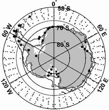
Data assimilation was performed using the Oregon State University Tidal Inversion Software (OTIS: http://www.oce.orst.edu/po/research/tide/index.html), which uses the representer approach to data assimilation (Reference Egbert, Bennett and ForemanEgbert and others, 1994; Reference Egbert, Bennett and Malonette-RizzoliEgbert and Bennett, 1996; Reference EgbertEgbert, 1997). A total of 37 tide-gauge stations lie in our model domain (Table 1), including coastal sea-level gauges and bottom pressure recorders, and gravimeter measurements on the Ross and Ronne Ice Shelves. Twelve of these records were excluded, 4 because of uncertainties in their quality, and 8 gravimeter stations on the Ross Ice Shelf which are used to provide independent validation of model performance in this region. Representers were located at each of the remaining 25 sites, and an additional 270 representers were located in the T/P data domain (north of ~66.2˚ S). Locations of all representers and the eight Ross Ice Shelf gravimeter records are shown in Figure 1. Note that the data south of the T/P data domain account for 510% of the total number of representers. Their influence on the final model is greater than this, however, because the model–data misfit is scaled by a prior error covariance map, which in turn depends on the amplitude of the tides in the prior model solution. Since the largest tidal amplitudes are found in the southern and western Weddell Sea and Siple Coast section of the Ross Sea (see Fig. 2), data from these regions have a significant influence on the final inverse solution. Nevertheless, most of the inverse model improvement relative to the forward model is due to the tight constraints imposed by the 270 T/P-based representer sites north of ~66.2˚ S.

Fig. 1. Representer and data locations for the CADA00.10 model. The T/P satellite radar altimetry measurements are all north of ∽66.2˚ S (indicated by the dashed line). The 270 representer locations within the T/P coverage area are shown as small dots. Asterisks indicate locations of non-T/P data records (Table 1) that are also used as representer sites in the assimilation. Solid squares on the Ross Ice Shelf show the locations of eight gravimeter records that are used in validating the tide models but are not used in the assimilation. Solid black contours indicate the 1000 and 3000 m isobaths, and the gray contour represents the ice fronts.
Fig. 2. Rms tide height (σζ) for the entire circum-Antarctic seas to 60˚ S. The thick white line is the SCAR 1993 ice-shelf edge. The black line is the 1000 m water-depth contour as a guide to the location of the continental slope.
Table 1. Tidal records used in model for assimilation or validation
As a measure of the efficacy of data assimilation, in Table 2 we present the root-mean-square (rms) error for the four major constituents, M2, S2, K1 and O1. These error estimates are calculated in the time domain, i.e. errors of both amplitude and phase are included in the calculations. We use two datasets, the 25 non-T/P sites used in the assimilation, and the eight gravimeter stations on the Ross Ice Shelf. Note that since the former dataset is used in the assimilation, improvements from the forward to the inverse solution are expected. In contrast, the gravimeter sites provide an independent check of the value of data assimilation as a dynamical means of data interpolation/extrapolation. With the exception of M2 on the Ross Ice Shelf, assimilation significantly improves the fit between the model and measurements. The fit of the inverse solution to the 25 assimilated sites, rms errors of 2–4 cm per constituent, is constrained by the choice of our expected error for each height measurement and our choice of a value for the OTIS parameter, σε, which essentially measures the relative role of dynamics and assimilated data in constraining the final solution. Overconstraining the inverse model to height data results in height fields that are bumpy, and unrealistic velocity fields and dynamic residual errors (the error forcing that is required to nudge the forward model solution to the inverse solution). Our choice of σε, which is chosen separately for each species (semi-diurnal and diurnal), is presently based on a combination of subjective tolerance for height field variability, and informal comparisons of model predictions with other data types such as current-meter data and satellite interferometry.
Table 2. Comparison of the rms error (in cm) between the modeled and measured tide heights for the four major tidal constituents, M2, S2, O1and K1
The comparison of forward and inverse model skills in Table 2 indicates that further improvements are required under the Ross Ice Shelf. In a study of Ross Sea tides that will be reported elsewhere, we show that assimilating the eight gravimeter records from the ice shelf significantly improves model performance as judged by model comparisons with SAR interferometry data from the Siple Coast (personal communication from I. Joughin, 2001).
The full model grids for both CATS00.10 and CADA00.10 can be obtained on CD-ROM (in ![]() form) from the first author.
form) from the first author.
Model Results
We characterize tidal-height variability by the standard deviation of the modeled tidal-height fields summed over all tidal constituents. This value, σζ, is given as a function of position (x; y) by
where hn is the height amplitude of the nth tidal coefficient. The typical magnitude of the tidal range (low to high tide) is ~2σζ. We also define a maximum height, ζmax, given by
i.e. the height when all 10 explicitly modeled constituents are in phase. We do not show maps of this value, but the distribution of ζmax(x; y)/σx; ζ(y) is narrow, with a mean value of ~2.4. The maximum peak-to-peak tidal range is ~2ζmax, or ~4–5 σζ. Slightly higher values are possible when the many minor tidal constituents are included in the summation in Equation (2) (see, e.g., Reference le Provost, Lyard, Molines, Genco and Rabilloudle Provost and others, 1997).
In the following subsections we summarize the distribution of σζ for three sectors of the Southern Ocean. Colorversions of the figures in this paper can be found at our web site, http://www.esr.org/antarctic.html.
Notes: The comparison is performed for each site in the time domain, i.e. both amplitude and phase errors between modeled and measured constituent values are used. The two datasets for which mean rms statistics are presented are: the 25 non-T/P data records that are included in the assimilation; and the 8 gravimeter records on the Ross Ice Shelf (RIS) that were not assimilated. Results are presented for the forward model, CATS00.10, and the inverse solution, CADA00.10.
Weddell and Bellingshausen Seas
Model values of σζ exceed 150 cm in the Weddell Seaunder sections of the Ronne–Filchner and Larsen Ice Shelves (Fig. 3a). The spring tide peak-to-peak range exceeds 7 m in the channel south of the Henry and Korff Ice Rises in the southern Ronne Ice Shelf. This prediction is consistent with gravimeter records from near the grounding lines of the Doake Ice Rumples and Rutford Ice Stream, and site S902 (Reference SmithSmith, 1991; Reference Doake and OerterDoake, 1992; Reference Robinson, Doake, Nicholls, Makinson and VaughanRobinson and others, 1996). The major semi-diurnal constituents, M2 and S2, dominate tide heights except near their amphidromic points close to the center of the Ronne Ice Shelf front.
Fig. 3. Close-up of rms tide heights (σζ ) for three sectors. Asterisks indicate locations of non-satellite tide-height records listed in Table 1. (a) Weddell and Bellingshausen Seas. The highest values of σζ in the southern Filchner–Ronne Ice Shelf are >180 cm south of the Henry and Korff Ice Rises (HKIR). The locations of tidal measurements at Ronne Entrance (R.E.) and the Rutford grounding line (Rutford G.L.) are indicated. (b)Ross Sea to Pine Island Bay (PIB). The highest values of σζ in the eastern Ross Ice Shelf are >80 cm along the Siple Coast. The locations of tidal measurements at McMurdo Sound and the Little America Station(LAS) are indicated. (c) East Antarctic sector including the AIS. The highest values of σζ in the southern AIS are ∽70 cm. The locations of tidal measurements at Beaver Lake (B.L.) on the western side of the AIS, the GPS measurements at the hot-water-drilling site (HWD) and the Mawson, Davis and Casey stations are indicated.
Our modeled tide heights in this region are acceptable for most present purposes, even without assimilation: in differential SAR interferograms (DSIs) from the front of the Ronne and Filchner Ice Shelves (Reference Rignot, Padman, MacAyeal and SchmeltzRignot and others, 2000), the typical error between the differential height signal in the DSIs and the same signal synthesized from the non-assimilative CATS model was about 10 cm. Tests in which we increased the benthic friction coefficient under the ice shelves, as a simple means to parameterize additional tidal-energy sinks, suggest that higher energy losses under the ice shelf further improve the fit of the CATS model to the ice-front DSIs, although at the cost of poorer fits to open-ocean data. The best fit was found for an under-ice drag coefficient of CD = 0.015, which is ~5 times greater than is typically used for benthic friction in ocean tide models. Reference Williams and RobinsonSmithson and others (1996) came to a similar conclusion: a higher value of CD under ice shelves is required to reproduce some data, particularly near the grounding line, but also at the expense of degrading agreement at open-water sites. While some of the additional energy loss can be attributed to turbulence generation at the ice-shelf base, other energy sinks are needed to explain this large value of CD. Possibilities include inelastic flexure in the grounding zone, non-linear transfers to other frequencies, and generation of baroclinic tides. Identifying and parameterizing these additional energy sinks under ice shelves is a priority for future studies.
Smaller values of σζ (~50 cm) occur in the Bellingshausen Sea. Three tidal stations, Faraday, Rothera and Ronne Entrance (Table 1), are available to test forward model performance in this region, and to constrain the inverse solution. In early versions of CATS, tides at Ronne Entrance (73.13˚ S, 72.53°W) were very poorly represented when the model was run with the ETOPO-5 global bathymetry grid, in which the cavity under the George VI Ice Shelf was 20m thick. The forward model performed much better, however, when the grid of d(x; y) was adjusted to agree with values based on seismic sounding transects across the George VI Ice Shelf (Reference MaslanyjMaslanyj, 1987). These transects showed that d exceeds 600 m in a trough that runs under the entire length of this ice shelf, providing a conduit for tidal energy flux around the eastern side of Alexander Island that was essentially closed with the ETOPO-5 grid.
Ross Sea to Pine Island Bay
Under the Ross Ice Shelf, σζ is ~60 cm, except for a small region of higher σζ (up to 140 cm) along the southern Siple Coast where Ice Streams A and C and Whillans Ice Stream enter the Ross embayment (Fig. 3b). Tides are predominantly diurnal except along the Siple Coast. However, the distribution of d in this area is poorly known, and even the grounding-line location is uncertain: recent satellite data suggest that the Crary Ice Rise is actually connected to the Siple Coast instead of being a separate feature as indicated in present coastline charts (Reference GrayGray and others, 2002).
Tidal records for the Ross Ice Shelf are mainly gravimeter time series obtained in the 1970s (Reference Williams and RobinsonWilliams and Robinson, 1980).With the exception of the Little America Station (LAS) point, these gravimeter data are not included in the data-assimilation runs discussed herein. The typical amplitudes for the two most energetic diurnal constituents, K1 and O1, are about 30–40 cm. The rms error for the unassimilated gravimeter points (Table 2) is about 4 and 5 cm, respectively, for K1 and O1, i.e. 10–20% of the true signal. Most of this error arises through phase errors: modeled diurnal amplitudes are within 2–3 cm of measured values. The weaker semi-diurnal constituents are very poorly represented in the model, even with assimilation of LAS and McMurdo Sound tide records. Both amplitude and phase errors are large. For one example, the S2 amplitude and phase at F9 (in the southeastern corner of the Ross Ice Shelf) is 11 cm and 142˚ from data, but 28 cmand187˚ from CADA00.10. The rms error resulting from this misfit is ~15 cm, with maximum values of ~22 cm. That is, the error in S2 alone can exceed our nominal requirement of ~10 cm for tidal prediction accuracy. The S2 constituent is difficult to predict because some of the S2 signal in data records is associated with ocean response to atmospheric radiational tides, and so is not modeled correctly by the shallow-water equations.
Three main factors contribute to the difficulty of modeling tides in the Ross Sea. First, T/P altimetry of the open-ocean surface is not available south of ~66.2˚ S, more than 1000 km north of the Ross Ice Shelf front. The T/P data provide the most rigorous constraint on the inverse model solution because of the good spatial coverage of the data in the northern part of our model domain. Second, d(x; y) under the Ross Ice Shelf is poorly known, and may also have changed significantly since the surveys in the 1970s (see Reference GrayGray and others, 2002). Third, no high-quality modern tidal records exist for the Ross Sea. The quality of the gravimeter records is unknown; hence, some of the difference between the model and the data may be due to data errors rather than model quality. (However, as we noted previously, assimilation of all the gravimeter sites does improve model comparisons with SAR interferometry estimates of tidal displacement.)
The value of σζ in Pine Island Bay (~~105°W) is 50–60 cm. Pine Island and Thwaites Glaciers are dynamic ice streams draining the West Antarctic marine ice sheet, and are believed to be presently out of dynamic equilibrium (Reference RignotRignot, 1998; Reference Wingham, Ridout, Scharroo, Arthern and ShumWingham and others, 1998). Tide modeling is important for this region, both to assess the possible role of tides in the loss of shelf ice and to remove tide-height variability for satellite sensing of trends in ice-shelf thickness. There are, however, no tide data and very few bathymetry data in this region, so even our data-assimilation model is poorly constrained at this time.
East Antarctica
Along most of the coast of East Antarctica, σζ is ~40–55cm (Fig. 2). However, under the Amery Ice Shelf (AIS) at the southern end of Prydz Bay, σζ increases to ~65 cm near the groundingline (Fig.3c). Tides in this sector are mixed diurnal– semi-diurnal. Tidal currents under the ice shelf are small, typically<5 cm s–1. With the exception of the AIS, much of the East Antarctic coastline lies close to the southern limit ofT/P altimetry coverage, unlike the southern portions of the major embayments of the Weddell and Ross Seas. Tidal-height predictions in this sector are therefore relatively reliable in our model, because of the assimilation of T/P data. As expected, due to the T/P constraints in CADA00.10, our model predictions for σζ at Mawson, Davis and Casey stations are close to the measured values. For the AIS, errors in our forward model (CATS00.10), as judged by time-series comparisons between short GPS records and model predictions, increase further south. These data are not, however, of sufficient duration to be assimilated in CADA00.10, and so can only be used for model validation studies. When tides at Beaver Lake (a tidal lake to the west of the ice shelf) and the hot-water drilling site (HWD-2000) near the northwestern corner of the AIS are assimilated, the rms errors between model predictions and the GPS data further south are slightly reduced. Much of the error may, however, be due to the exclusion of non-tidal sources of height variability, and so would not be removed even if the tidal model were perfect.
An Example Of Tide-Model Application To Satellite Data
Satellite orbit repeat periods (ΔT) are long compared with tidal time-scales, and so the satellite data undersample tidal variability. Tidal energy appears in the satellite record at an aliasing frequency that falls between 0 and 1/(2ΔT). If the aliasing frequencies for the major constituents are separable during a mission life, then tidal information can be retrieved from the satellite records. This is true for the T/P satellite, whose orbit was designed specifically for tidal retrieval (Reference Parke, Stewart, Farless and CartwrightParke and others, 1987). For other satellites, however, this is not the case. Reference SmithSmith (1999) and Reference Smith, Ambrosius and WakkerSmith and others (2000) compared aliasing periods for GEOSAT, the European Remote-sensing Satellite (ERS) and T/P, and found that several problems arise. First, a constituent may be effectively frozen; that is, its alias period is long compared with the satellite’s mission life, or even infinite. In this case, regardless of how large the constituent amplitude is, the recorded variability of that constituent is negligible during a mission. Second, two or more constituents may be aliased to nearly the same frequency, and so cannot be separated from each other. Third, constituents may be aliased to other frequencies at which non-tidal energy may be present. The most significant source of non-tidal energy is the annual response to cycles in oceanic or atmospheric conditions. The diurnal constituents K1 and P1 in the 35 day repeat phases of the ERS missions are both aliased to ~1year periods and so cannot be separated from each other or from non-tidal, annual variability.
To demonstrate the aliasing problem, we show a 1year time series of predicted tide heights for the point 71.5˚ S, 70°E on the AIS, and the same time series sampled by the GLAS ~8 day repeat Verification Phase (Fig. 4). We show a full year of predictions, even though the Verification Phase is only planned to be 3 months long, to demonstrate the range of possible outcomes from a short mission. The apparent quasi-annual cycle in the GLAS time series arises because two of the four largest semi-diurnal tides, S2 and K2, have aliasing periods of ~ 1year. Another energetic constituent, the diurnal K1, has an aliasing period of about 2 years. During the first 100 days, GLAS sees significant short-period variability associated with the tide. From day 100 to day 200 the trend in height is downward, until it recovers in the last half of the year but with reduced short-period variability. If this entire signal was interpreted as being non-tidal, the apparent height change (Δh) over 3 months of data collection could be as large as 60 cm. If the GLAS time series was corrected with a tidal model, Δh would be smaller but would still contain the aliased signal of the tide-model error. Thus, without an accurate tide model, tidal-height variability seen in the GLAS data may be misinterpreted as long-time-scale, non-tidal, geophysical variability.
Fig. 4. Example of satellite aliasing problem. The thin gray line is the predicted hourly tide height for the point 71.5˚ S, 70°E on the AIS. The thick black line is the same tidal time series sampled at the GLAS sampling frequency during the 8 day repeat, Verification Phase of the ICES at mission. This phase will only last for 3 months, but we show 1year of prediction to demonstrate the range of possible outcomes for an aliased time series that is shorter than the aliasing periods of major constituents.
Another potential source of error over ice shelves that may be significant in satellite altimeter data is the inverse barometer effect (IBE). The isostatic response of the ocean surface to changing air pressure (Patm) is a depression of ~1cm for each 1mbar increase in Patm (Reference GillGill, 1982, p. 337). A pressure anomaly of ~30mbar associated with a typical polar low therefore leads to a ~30 cm increase in sea level. There is some evidence from differential SAR interferometry that the IBE can be an important component of the residual height-change signal after tides have been removed (Reference Rignot, Padman, MacAyeal and SchmeltzRignot and others, 2000).
Conclusions
We have presented a new tide model for the Antarctic ice shelves and seas south of 58˚ S. Data assimilation was used to constrain the model to better agreement with measurements of tide height. Typical peak-to-peak tidal ranges under most ice shelves fringing Antarctica are 1~–2m. This can increase to 2–4m at spring tides, and occasionally exceeds 6 m, notably under the south of the Filchner–Ronne Ice Shelf (FRIS) in the southern Weddell Sea. Tides provide the major short-period signal that will be detected by satellite-based techniques such as SAR and laser altimetry. These instruments can detect height variability of ~5 cm or smaller, yet we cannot provide tidal predictions at accuracies better than 10–20cm for several critical segments of the Antarctic ice-shelf area, notably the southern FRIS and the eastern side of the Ross Ice Shelf. Thus, the quality of tide models is presently one of the factors preventing the full exploitation of these datasets.
Forward tide models based on the shallow-water equations can be improved by increasing the sophistication of the model physics and the accuracy of the water-column thickness grid. In an attempt to address the former requirement, we are currently investigating adding parameterizations for tidal energy loss to baroclinic tide generation, following Reference Jayne and LaurentJayne and St. Laurent (2001), and changing the bottom drag coefficient to improve model fit to various datasets. We have found that increasing the parameterized tidal energy dissipation under ice shelves improves model skill along the Ronne and Filchner ice fronts when compared to displacements observed in DSIs (Reference Rignot, Padman, MacAyeal and SchmeltzRignot and others, 2000). However, the additional energy loss implied by this parameterization is much larger than one would expect from extra turbulence production at the ice-shelf base. This suggests that there is at least one more major physical mechanism for energy loss under ice shelves. Possible energy sinks not accounted for in our present forward model include inelastic flexure in the grounding zone, baroclinic tide generation, and/or transfer of tidal energy to other harmonics and terms through non-linear interactions, especially in the shallow water near the grounding zones.
The alternative approach to improving tide modeling, using an inverse technique such as data assimilation, requires that we increase the number of tidal records for assimilation. Satellite altimetry aside, most new data will consist of bottom pressure sensors moored in the ocean near the ice fronts, or static GPS on ice shelves controlled with nearby GPS on bedrock (e.g. Reference King, Nguyen, Coleman and MorganKing and others, 2000). In this case, care should be taken to obtain the ice-shelf records well away (>10 km) from the grounding line and shear margins, since the tide models presently do not include the glacial rheology needed to model tide-forced displacements within the flexural boundary layer. Models can predict phase and relative amplitude information closer to the grounding line but will overestimate absolute amplitude (Reference Riedel, Nixdorf, Heinert, Eckstaller and MayerRiedel and others, 1999). Ideally, the new measurements would be of long duration (e.g. 1year), allowing good resolution of the major tidal constituents. However, shorter records are still useful: records of 30 days or longer can be analyzed for the major tidal constituents, and shorter records can be used for model validation. To our knowledge, the only current plan for significant tidal data collection is for the Amery Ice Shelf. Other areas, particularly the outlets of the major West Antarctic ice streams along the Siple Coast and Pine Island Bay, require new tide measurements.
One additional source of ice-shelf height variability that is not accounted for in our tide model is the IBE, which, as we discussed above, causes a change of ~1cm per 1mbar change in atmospheric pressure. Since typical pressure anomalies for polar low-pressure systems are ~30mbar, an IBE response of ~30 cm change in sea level is possible. This must be considered when attempting to de-tide satellite-derived measurements of ice-shelf heights.
Acknowledgements
The ocean tidal modeling was supported by grants to Earth& Space Research from the U.S. National Science Foundation Office of Polar Programs (OPP-9896041) and NASA (NAG57790). Funding for H.A.F. was provided by NASA grant NAS599006 to GLAS Team Member J.-B. Minster. Work on the Amery Ice Shelf was supported by grants to R.C. from the Australian Research Council and the Antarctic Science Grant (ASG) scheme. Tidal sea-level analyses for Mawson, Davis and Casey stations and Beaver Lake were supplied by the National Tidal Facility, The Flinders University of South Australia, copyright reserved. We thank the reviewers for their valuable comments on the manuscript.
Appendix
The CATS/CADA Depth Grid
Our 1/4°61/12˚ model grid of d(x; y) is based on ETOPO-5 (NOAA, 1988). Smith and Sandwell (1997) have developed a high-resolution depth grid for regions north of 72˚ S, using gravity anomalies obtained from satellite altimeter heights to interpolate water depth between ship-track depth soundings. However, we have not yet developed a satisfactory scheme for merging this grid with our grid for regions south of 72˚ S, and so have not yet implemented this improvement. Instead, we have updated several areas of specific interest using local depth grids. For the open Weddell Sea, we use a grid developed by Robertson and others (1998), which has been updated with depth data for the southwestern Weddell Sea acquired during the 1998 Ronne Polynya Experiment (ROPEX-98) (Nicholls and others, 1998). For the open Ross Sea, we use a grid generated from data acquired from the U.S. National Geophysical Data Center (NOAA,1992). The resultant map of water depth for the open-water section of the Ross Sea is similar to that presented by Reference Brancolini, Cooper, Barker and BrancoliniBrancolini and others (1995). For the Amundsen Sea, including Pine Island Bay, we use ETOPO-5, but replace shallow shelf depths in ETOPO-5 with a more typical depth of 400 m.
Water-column thickness for the ocean cavities under the major ice shelves was obtained from various sources. Gridded water-column thickness data for the Filchner– Ronne Ice Shelf were obtained from Reference Johnson and SmithJohnson and Smith (1997), and those for the Ross Ice Shelf were provided by D. Holland (personal communication, 1999) based on the measurements reported by Reference Greischar and BentleyGreischar and Bentley (1980). The Ross Ice Shelf cavity geometry was updated using the 1993 SCAR coastline (SCAR, 1993). Depths for the George VI Ice Shelf were obtained from Maslanyj (1987). For the AIS, d(x; y) was obtained from Williams and others (1998), and the ice shelf was extended further south based on results of hydrostatic calculations (Fricker and others, in press). For all other ice shelves, d(x; y) was taken from ETOPO-5.