


Introduction
The major aim of the Global Land Ice Measurements from Space (GLIMS) initiative is to generate a global snapshot of digital glacier outlines from satellite data and make them available to the wider scientific community via the internet (Reference Khromova, Dyurgerov and BarryKargel and others, 2005; Reference Rignot, Rivera and CasassaRaup and others, 2007b). Given the declining glacier mass on a global scale (Reference MihalceaLemke and others, 2007; WGMS, 2007, 2008), the increasing importance of glacier meltwater as a water resource in the dry season in areas such as the Himalaya (Reference Surazakov and AizenSingh and others, 1997; Reference Sun, Ranson, Kharuk and KovacsSingh and Jain, 2002; Reference Singh, Jain and KumarSingh and Bengtsson, 2004; Reference Bamber and RiveraBarnett and others, 2005) and the Andes (Reference Bradley, Vuille, Diaz and VergaraBradley and others, 2006), as well as the contribution of alpine glaciers to global sea-level rise (Reference Aniya, Sato, Naruse, Skvarca and CasassaArendt and others, 2002; Reference RöhlRignot and others, 2003; Reference RaupRaper and Braithwaite, 2006; Reference Narama, Kääb, Kajiura and AbdrakhmatovMeier and others, 2007), global glaciological data are required for four main reasons:
1. The World Glacier Inventory (WGI) was compiled from aerial photography, maps and satellite imagery acquired during the 1960s and 1970s and is not complete with respect to detailed glaciological information (World Glacier Monitoring Service, 1989). Furthermore, glaciers in the WGI database are represented by point data rather than glacier outlines, making change detection for individual glaciers nearly impossible.
2. Data for the WGI were compiled mostly during the 1960s, 1970s and 1980s. Since that time period, major changes have taken place in glaciers all over the world (Reference Barnett, Adam and LettenmaierBarry, 2006; Reference Khromova, Osipova, Tsvetkov, Dyurgerov and BarryKaser and others, 2006; Reference MihalceaLemke and others, 2007). This means that there is an urgent need to update the global glacier database, as mentioned in the strategy of the Global Terrestrial Network for Glaciers (GTN-G) (Reference Haeberli and EpifaniHaeberli, 2006).
3. Complete detailed glacier parameters such as glacier area, length, elevation, hypsography and ice volume in particular are needed for those glacierized regions that are currently missing from global mass-balance records or have only preliminary data in the WGI, such as the Arctic, Himalaya and Patagonia (Reference BraithwaiteBraithwaite, 2002; Reference Duncan, Klein, Masek and IsacksDyurgerov and Meier, 2005; WGMS, 2007). Moreover, coupled models for assessing the impact of climate change on glacier evolution (e.g. Reference HaeberliGregory and Oerlemans, 1998; Raper and others, 2000; Reference RaupRaper and Braithwaite, 2006) require detailed glacier parameters, in particular glacier area and hypsography.
4. There is a need to incorporate glaciers and ice caps near, or adjacent to, Greenland and Antarctica into global mass-balance and sea-level estimates (Reference RaupRaper and Braithwaite, 2006; Reference Raup, Racoviteanu, Khalsa, Helm, Armstrong and ArnaudRahmstorf, 2007).
On a global scale, glacier outlines can be derived using automated classification algorithms from multispectral satellite data (e.g. Reference Paul and L.M.Paul and others, 2002; Reference Paul, Huggel and KääbPaul and Kääb, 2005), as recommended in the GTN-G (Reference Haeberli and EpifaniHaeberli, 2006). The advantages of using remote sensing for glacier delineation are:
1. Sensors such as the Landsat Thematic Mapper (TM) have a relatively large swath width (185 km) and cover large areas with a medium spatial resolution (~30 m). Since the end of 2008, the entire United States Geological Survey (USGS) Landsat Archive, containing 35 years of nearly complete global coverage data from the Landsat TM and Landsat Enhanced TM Plus (ETM+) sensors, has been available at no charge from the USGS (http://landsat.usgs.gov/).
2. For regional-scale studies, satellite imagery has been available from the Advanced Spaceborne Thermal Emission and Reflection Radiometer (ASTER) sensor since 2000. The adequate spatio-temporal resolution (16 days revisit time, 60 km swath width, 15m spatial resolution in the visible and near-infrared (VNIR)), high spectral resolution (14 bands), low cost (free for GLIMS), near-global coverage and the capability of acquiring stereo imagery make ASTER a suitable sensor for monitoring glacier parameters, including velocity fields and other applications (Reference Kaser, Cogley, Dyurgerov, Meier and OhmuraKääb and others, 2003; Reference Raper, Brown and BraithwaiteRacoviteanu and others, 2008b).
3. Automated methods for multispectral glacier classification have been developed and tested in the past decade using Landsat TM and ASTER imagery (Reference BarryBayr and others, 1994; Reference Singh and JainSidjak and Wheate, 1999; Reference Paul and L.M.Paul, 2002; Reference Paul and L.M.Paul and others, 2002; Reference Kaser, Cogley, Dyurgerov, Meier and OhmuraKääb and others, 2003, Reference Kääb, Paul, Maisch, Hoelzle and Haeberli2005; Reference Paul, Huggel and KääbPaul and Kääb, 2005; Reference Raper and BraithwaiteRacoviteanu and others, 2008a). These methods are simple, robust and accurate for detection of clean to slightly dirty glacier ice and fresh snow (Reference AlbertAlbert, 2002; Reference Paul and HaeberliPaul, 2007).
4. Remote-sensing-derived glacier outlines combined with digital elevation models (DEMs) in a geographic information system (GIS) are used to derive topographic glacier inventory parameters such as hypsometry, minimum, maximum and mean elevations in an efficient manner (Reference Larsen, Motyka, Arendt, Echelmeyer and GeisslerKlein and Isacks, 1996; Reference DozierDuncan and others, 1998; Reference KääbKääb and others, 2002; Paul and others, 2002; Reference Paul and HaeberliPaul, 2007).
5. Digital elevation data from remote sensing are increasingly available for conducting glacier change studies at various spatial scales. The global DEM derived from ASTER data (GDEM) was released in July 2009 and is freely available from the Japanese Earth Remote Sensing Data Analysis Center (ERSDAC) at http://www.gdem.aster.ersdac.or.jp/ and from NASA’s Land Processes Distributed Active Archive Center (LP DAAC) at: https:// wist.echo.nasa.gov/~wist/api/imswelcome/. Near-global (60˚N to 57˚ S) elevation datasets at ~90m spatial resolution are available from the Shuttle Radar Topography Mission (SRTM), flown in February 2000 (Reference Racoviteanu, Williams and BarryRabus and others, 2003; Reference Eckert, Kellenberger and IttenFarr and others, 2007). Various versions of the SRTM data are available at no cost over the internet. The ‘unfinished’ product is available from the USGS (http://srtm.usgs.gov/data/obtainingdata.php) but it contains data voids, unedited coastlines, spurious values and some geolocation shifts. The latest version of the SRTM data (‘finished’ version 3/4) available from the Consultative Group for International Agriculture Research – Consortium for Spatial Information (CGIAR-CSI) (e.g. http://www.ambiotek.com/topoview/) is a hydrologically sound DEM where data voids were filled by interpolation. However, the interpolated regions in the ‘finished’ version of the SRTM may be inaccurate, so the ‘unfinished’ version can be used to mask these regions out for further analysis.
The GLIMS initiative
Based on this increasingly available stock of satellite imagery suitable for global glacier monitoring from space, mapping activities within the GLIMS initiative became widespread (Reference Khromova, Dyurgerov and BarryKargel and others, 2005). As of August 2009, the GLIMS Glacier Database hosted at the National Snow and Ice Data Center (NSIDC) in Boulder, CO, USA, contains digital vector outlines from approximately 83 000 glacier entities, covering an area of 262 000 km2. Glacier outlines can be downloaded at no cost from the GLIMS website (www.glims.org). The website also has several tools for data query and visualization Reference Rignot, Rivera and Casassa(Raup and others, 2007a). The glacier delineation techniques applied by individual GLIMS regional centers vary from full manual glacier delineation to various automated techniques based on multispectral classification of ice and snow. A number of GLIMS analysis comparison experiments (GLACE) have demonstrated that the automated methods produce very similar results for sunlit clean ice and snow, while the analyst’s interpretation in the delineation of more challenging regions (debris, shadow and lakes) may differ strongly (Reference Rignot, Rivera and CasassaRaup and others, 2007b). In particular, the methodological interpretation of a glacier as an entity (ice divides, split tributaries and compound glaciers) varies widely, prompting the need for standardized methods. Two of the tutorials generated by the GLIMS team to guide the interpretation of the satellite images and to provide consistency among regional centers are: the GLIMS Analysis Tutorial (B. Raup and S. Khalsa, http://glims.org/MapsAndDocs/assets/GLIMS_Analysis_Tutorial-a4.pdf; hereafter GLIMS Analysis Tutorial) and the Illustrated GLIMS Glacier Classification Manual (F. Rau and others, www.glims.org).
Several workshops and meetings have been held within the GLIMS initiative to discuss technical and methodological challenges of glacier mapping and to propose possible solutions. The most recent of these workshops was held during 16–18 June 2008 at the NSIDC. This GLIMS workshop focused on advances and the current state of knowledge related to glacier studies using remote sensing. This paper summarizes the major results of this workshop with an emphasis on definitions, methods and recommendations for satellite-data processing. These are relevant issues for deriving glacier inventory data from spaceborne sensors on a global scale. While the list of proposed methods and recommendations is not comprehensive, our goal here is to provide a starting point for the regional centers in terms of documentation on possible pitfalls in remote-sensing methods for glaciers, along with potential solutions. The following section introduces the workshop topics, remaining challenges and definitions.
GLIMS Workshop Topics, Challenges and Definitions
Workshop topics
During the first 2 days of the 2008 GLIMS workshop, two key topics were addressed by a total of 17 oral presentations and six focus groups: (a) glacier delineation (day 1); and (b) DEM generation and analysis (day 2). Specifically, oral presentations and working groups focused on algorithm development and comparison on the following topics:
1. mapping clean ice and lakes;
2. mapping ice divides;
3. mapping debris-covered glaciers;
4. assessing changes in glacier area and elevation through comparisons with older data;
5. DEM generation from satellite stereo pairs;
6. accuracy and error analysis.
Day 3 of the workshop was dedicated to summaries and discussion on the topics addressed during the first 2 days. The overarching goal of this workshop was to achieve consensus on algorithms and procedures used for glacier analysis, and to prepare a set of recommendations that can be used by the GLIMS regional centers to avoid inconsistencies in the various glacier datasets included in the GLIMS database. All workshop presentations are listed in Table 1 and are referred to in the text as numbers (e.g. [1] corresponds to reference 1 in Table 1), to distinguish them from bibliographic references.
Table 1. A selection of oral presentations and topics from the GLIMS workshop held during 16–18 June 2008 at the NSIDC. Presentations point to studies cited in the paper
Challenges
One aim of this contribution is to describe the most relevant aspects pertaining to glacier outlines derived from satellite data. The focus is on proposing simple, robust and established techniques that work well in most cases. We acknowledge the fact that several special cases, such as debris-covered glaciers, rock glaciers and frozen/turbid lakes, might not be solved with the methods proposed below, and need special attention. Further development of algorithms is ongoing and may provide ways to overcome some of the current problems in the future. However, these are not all described here in detail. The present discussion focuses on remaining challenges with mapping glacier outlines and deriving basic glacier parameters (mostly glacier area and elevation). Additional glacier parameters that can be derived from spaceborne sensors (e.g. mapping of snowlines, flow velocity, debris thickness, glacier lake temperatures and turbidity) are not discussed at length here. Instead, the reader is directed to a number of studies published specifically on these topics: glacier velocity (Reference Berthier, Arnaud, Baratoux, Vincent and RémyBerthier and others, 2005; Reference Kääb, Paul, Maisch, Hoelzle and HaeberliKääb, 2005), glacier lake temperature (Reference Scherler, Østrem and WallénWessels and others, 2002) and debris thickness (Reference PaulMihalcea and others, 2008). A thorough discussion on most remote-sensing techniques for glacier mapping can be found in Reference Bishop, Hickman and ShroderBishop and others (2000), Reference Arendt, Echelmeyer, Harrison and LingleBamber and Kwok (2004), Reference Kayastha, Takeuchi, Nakawo and AgetaKääb and others (2005), Reference BamberBamber (2006) and Reference Bamber and KwokBamber and Rivera (2007).
In mapping glaciers from satellite imagery within a specific region, three of the most important questions are: (1) Which sensor has the best data for glacier mapping of our region? (2) Which sensor should be used in a particular region? and (3) How can individual glacier entities be identified? While (1) and (2) are related to technical issues and data availability that vary widely with the investigated region and the mapping conditions (e.g. the presence of clouds and snow), (3) is a methodological issue that needs further guidance and is less clear in most cases. Here we present semi-automated methods for mapping clean and debris-covered glacier ice, as well as for delineating ice divides (glacier drainage basins) using available datasets. In many cases, the analyst may also be interested in comparing the new glacier extents with previous assessments derived from other data sources, such as different sensors or, most commonly, older topographic maps. Therefore, this overview includes a discussion on glacier change analysis (area and elevation changes). As DEMs constitute an essential tool for extracting glacier parameters such as length, mean elevations, slope and aspect, as well as for debris-cover mapping and analysis, we also discuss techniques for DEM generation from stereo satellite imagery and give general recommendations for DEM quality assessment.
Definitions
Before presenting techniques for glacier mapping, it is important to be clear about what should be mapped. The answer to the simple question ‘What is a glacier?’ varies with the purpose of the investigation. We rely on definitions developed within the context of the GLIMS project and further discussed during the June workshop. While these definitions are based on other official documents like the UNESCO guidelines for the compilation of the WGI (Reference PaulMüller and others, 1977), they were adapted for the purpose of satellite-based mapping.
GLIMS definition of a glacier
The GLIMS definition of a ‘glacier’, tailored to remote sensing and compliant with the World Glacier Monitoring Service (WGMS) standards, states that: ‘A glacier or perennial snow mass, identified by a single GLIMS glacier ID, consists of a body of ice and snow that is observed at the end of the melt season, or, in the case of tropical glaciers, after transient snow melts. This includes, at a minimum, all tributaries and connected feeders that contribute ice to the main glacier, plus all debris-covered parts of it. Excluded is all exposed ground, including nunataks. An ice shelf shall be considered as a separate glacier’ (GLIMS Analysis Tutorial).
The following selected points from the explanation section should also be mentioned:
1. Bodies of ice above the bergschrund that are connected to the glacier should be considered part of the glacier, because they contribute snow (through avalanches) and ice (through creep flow) to the glacier.
2. A tributary in a glacier system that has been treated (and named) historically as a separate glacier should be included as part of the glacier into which it flows.
3. A stagnant ice mass that is still in contact with a glacier is part of the glacier, even if it supports an old growth forest.
4. If snowfields are identifiable, they should be disconnected from the main glacier. For hydrological purposes, they can be included in the GLIMS Glacier Database under a separate GLIMS glacier ID, but they must be marked as a snowfield.
5. Lateral glacier outlines that might be hidden by seasonal snow or by avalanches should be labeled as preliminary, or even the entire glacier can be excluded. Ice avalanche cones below a glacier terminus (dry-calving) are not part of the glacier.
Debris-covered glaciers
Debris cover on a glacier varies with thickness, presence or absence of dead ice, type of rock, thermal resistance of the material, etc. (e.g. Reference PaulMihalcea and others, 2008). Given the high variability in debris characteristics, an attempt to present a standardized definition of debris-covered ice is difficult. Debris on the glacier tongues refers to material incorporated into a glacier by mass-wasting processes, entrainment of subglacial debris and meltout of englacial debris. On a typical debris-covered glacier, such as Khumbu Glacier, Nepal Himalaya, the thickness of the debris ranges from 0m at the boundary with clean ice to up to several meters at the glacier snout (Conway and Rasmussen, 2000; Reference Klein and IsacksKayastha and others, 2000; Reference Taschner and RanziTakeuchi and others, 2000). Special cases which do not necessarily fit this category include: thermokarst debris-covered tongues on Tana Glacier, Chugach Mountains, Alaska, USA, and Malaspina Glacier, Alaska, where active debris-covered ice is covered by vegetation [1]; the old, weathered and dirty calving margin of Tasman Glacier, New Zealand (Reference Schiefer, Menounos and WheateRöhl, 2008), wet debris cover, as well as ice covered completely or partly by debris, where only some patches of ice are visible. Such ‘special cases’ must be treated separately. All debris-covered parts of the glacier should be mapped if possible.
Rock glaciers are sometimes difficult to distinguish from debris-covered glaciers in medium-resolution satellite imagery. Rock glaciers differ from debris-covered glaciers mainly by a much smaller size and a missing accumulation area. They often reach further down in elevation and their typical ridge-and-furrow surface structure and steep fronts result in a characteristic illumination pattern that can be identified on satellite scenes in most cases. We recommend that rock glaciers be included as a separate category in a glacier inventory when they are easily identified and properly delineated.
Ice divides
Ice divides are used to define the glacier as an individual entity in a hydrologic sense. This implies that connected units must be separated in the accumulation area where they drain into different basins. The separation of tributaries is more delicate as their connectivity can change over time. From this point of view it makes sense to start with the oldest available datasets (e.g. Little Ice Age extent as mapped from trimlines). According to the GLIMS Analysis Tutorial:
1. If there is no flow between separate parts of a contiguous ice mass, the two parts should, in general, be treated as distinct units, separated at the topographic divide. However, for practical purposes, such an ice mass may be analyzed as a unit at the analyst’s discretion, if delineation of the flow divides is impossible or impractical.
2. Any steep rock walls that avalanche snow onto a glacier but do not retain snow themselves should not be included as part of the glacier.
Available/Proposed Methods
Glacier mapping: clean ice and glacier lakes
Multitemporal satellite imagery from the Landsat TM and ETM+, Système Probatoire pour l’Observation de la Terre (SPOT) and ASTER sensors has been used for automated glacier mapping within the context of the GLIMS initiative in the Swiss Alps (Reference KargelKääb and others, 2002; Reference Paul, Kääb, Maisch, Kellenberger and HaeberliPaul and others, 2002), central Asia (Reference KrupnikKhromova and others, 2003,Reference Kulkarni2006; Reference Svoboda and PaulSurazakov and Aizen, 2006; Reference Aizen, Kuzmichenok, Surazakov and AizenAizen and others, 2007; Reference BolchBolch, 2007), the Peruvian Andes (Reference Gregory and OerlemansGeorges, 2004; Reference Raper and BraithwaiteRacoviteanu and others, 2008a) and the Himalaya (Reference Bolch, Kamp, Kaufmann and SulzerBolch and Kamp, 2006; Reference Bolch, Buchroithner, Pieczonka and KunertBolch and others, 2008) among others. Most of the papers presented at the GLIMS workshop dealt with glacier mapping algorithms from Landsat and ASTER. Here we present an overview of various methods for automated delineation of clean to slightly dirty glacier ice, with advantages and disadvantages of each algorithm. A more detailed review and comparison of band ratio techniques is provided by Reference Paul, Kääb, Maisch, Kellenberger and HaeberliPaul and others (2002), Reference Paul, Huggel and KääbPaul and Kääb (2005), Reference Paul and HaeberliPaul (2007) and Reference Raper, Brown and BraithwaiteRacoviteanu and others (2008b).
Automatic delineation of clean glacier ice relies on the high reflectivity of snow and ice in the VNIR wavelengths (0.4–1.2 μm) compared with a very low reflectivity in the shortwave infrared (SWIR; 1.4–2.5 μm) (Dozier, 1989; Reference Rivera and CasassaRees, 2006). In the absence of clouds, snow and ice are distinguished from the surrounding terrain using the VNIR bands from the various sensors available. Commonly used techniques such as TM3/TM5, TM4/TM5, the normalized difference snow index (NDSI) (Reference Hall, Bayr, Schöner, Bindschadler and ChienHall and others, 1995) and other methods using band ratios take advantage of the spectral uniqueness of snow and ice in the SWIR wavelengths to separate them from non-glacier areas such as rock, soil or vegetation (Reference BarryBayr and others, 1994). Other simple methods include: manual delineation based on visual interpretation; qualitative digital thresholding based on spectral reflectance (e.g. Reference Schiefer, Menounos and WheateRott, 1994); and linear/non-linear functional boundaries for supervised hard classifications (e.g. Reference Andreassen, Paul, Kääb and HausbergAniya and others, 1996).
Several presentations at the GLIMS workshop illustrated techniques for automatic extraction of clean to slightly dirty glacier ice. Three studies [3–5] used Landsat imagery to delineate glaciers over large regions in Norway, western Canada and Baffin Island, respectively. The TM3/TM5 ratio with a threshold of 2.0 (TM3/TM5 >2.0 = ice/snow) yielded satisfactory results for Norwegian glaciers where debris-covered ice is sparse (Reference Andreassen, Paul, Kääb and HausbergAndreassen and others, 2008). An area cutoff of 0.01 km2 and a 3 x3 median filter were applied to obtain glacier outlines for the Jotunheimen region (Fig. 1). Similar methods were employed by Bolch and others [4] to map the glaciers of British Columbia and Alberta (Bolch and others, in press) (Fig. 2). Racoviteanu and others [6, 7] illustrated the use of the NDSI in the Sikkim Himalaya, India, and the Cordillera Blanca, Peru. These studies emphasized the need to choose the threshold manually depending on the scene characteristics (e.g. haze, sun position and topography). For example, for Sikkim, the threshold chosen was 0.7 (NDSI > 0.7 = snow/ice) (Reference Raper, Brown and BraithwaiteRacoviteanu and others, 2008b), but for Cordillera Blanca the suitable threshold was 0.5–0.6 (Reference Raper and BraithwaiteRacoviteanu and others, 2008a). The NDSI algorithm correctly classified the clean ice in these two areas, including most of the ice in shadow (Fig. 3), and also masked out clouds. However, all band ratio algorithms fail to identify debris-covered ice. Paul [5] further provided a thorough comparison of various techniques, including band ratios TM3/TM5, TM4/TM5, NDSI (TM2 – TM5)/(TM2 + TM5), as well as a median filter and dark object subtraction (DOS) for Baffin Island (cf. Reference Paul, Huggel and KääbPaul and Kääb, 2005). For this region, Paul reports the TM 3/5 ratio with an additional threshold in TM1 to be a robust, simple and accurate method, partly even better then manual delineation (i.e. not generalized and consistent for the entire scene). An advantage of this method is that clean ice can be identified even under (optically) thin clouds and in shadow regions. Molnia and others [1] used various masks based on image ratios and thresholding of digital numbers (DN) to construct a glacier inventory of Afghanistan using ASTER and Landsat-7 ETM+ imagery from 2001 to 2004. The rather complex classification scheme also distinguishes between snow and ice, but glacier outlines are of the same quality compared with the simpler methods. For delineation of water bodies, some studies proposed the following: using the normalized difference water index (NDWI) [4]; using glacial lake color to aid classification schemes such as band ASTER 1/3 ratio and band 3 intensity [2]; and other new techniques such as sub-pixel mapping using ASTER imagery (Reference Zhang, Lin, Liu and ShiZhang and others, 2004). The accuracy of the glacier outlines derived from image classification using automated methods is generally estimated to be one pixel in most accuracy studies (Reference CongaltonCongalton, 1991; Reference Zhang and GoodchildZhang and Goodchild, 2002). However, the accuracy estimates may vary widely by region depending on the quality of the images, the methods used and the presence of debris-covered glaciers.
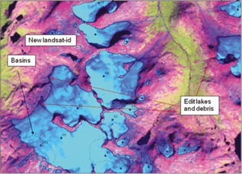
Fig. 1. The new glacier inventory for Jotunheimen, Norway, is based on Landsat TM and ETM+ imagery using a TM3/TM5 band ratio [3].The false-color composite (FCC) with bands 5, 4, 3 (as RGB) displays glaciers in light blue–green and also shows drainage divides, edited lakes and internal IDs of the glaciers finally selected.
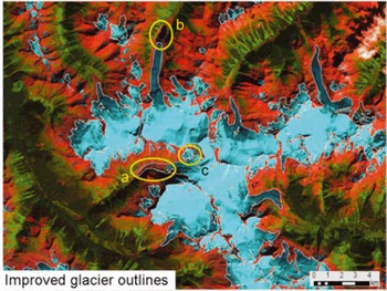
Fig. 2. Results of the western Canada glacier inventory based on Landsat scenes using the TM3/TM5 band ratio. Labels point to: (a) debris cover delineated manually; (b) proglacial lake edited manually; and (c) ice divides that are different in the glacier inventory from the Terrain Resource in Management (TRIM) program (http://ilmbwww.gov.bc.ca/bmgs/pba/trim) [4]. Clouds (white) are clearly recognizable in the FCC.
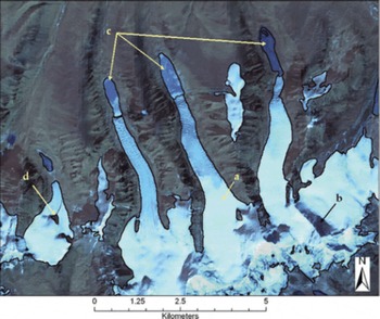
Fig. 3. Results of the classification algorithm for clean ice in northern Sikkim/China from 2001 ASTER imagery. Arrows point to: (a) clean snow and ice classified correctly; (b) shadowed glacier classified correctly; (c) proglacial lakes misclassified as glacier; (d) internal rock correctly delineated (reproduced from Reference Raper, Brown and BraithwaiteRacoviteanu and others, 2008b).
Challenges
While the above presentations illustrated the effectiveness of NDSI and single-band ratios (such as TM3/TM5 and TM4/ TM5) for fast glacier mapping over large areas, there remain challenges in regions with shadow, clouds, seasonal snow, turbid/frozen/multi-hued proglacial lakes and debris cover. Many presentations in the GLIMS workshop pointed to these challenges. For example, three studies [4, 5, 7] discussed problems in regions with clouds, late-season snow, perennial ice, proglacial/frozen lakes, regions with crevasses, dark (polluted) ice in shadow and debris cover (Figs 3–5). Figure 4 also indicates regions that are not accurately classified with the TM3/5 ratio (polluted bare ice in shadow and thicker debris cover). Figure 5 indicates the subtle differences in hue for ice-covered lakes compared with flat ice caps which can be present in some regions. In most studies, turbid or frozen glacier lakes and debris-covered glaciers were delineated manually using color composites from various VNIR and SWIR band combinations (Figs 2 and 5). Recommendations/ possible solutions with respect to mapping of shadow, clouds, seasonal snow, and turbid/frozen/multi-hued proglacial lakes are briefly presented below. Challenges related to debris-cover mapping were given special consideration in the GLIMS workshop by the working groups and are addressed in a separate section of this paper.
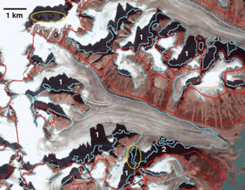
Fig. 4. Mapping accuracy of the TM3/TM5 ratio method in a challenging region near Penny Ice Cap on Baffin Island, Canada [5]. The light-blue lines show the glacier outlines as originally mapped, red lines indicate the glacier basins and yellow circles denote regions that have not been mapped correctly. The numbers indicate: 1 – snow and ice in shadow; 2 – bare rock in shadow; and 3 – snow couloirs.
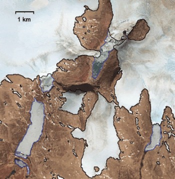
Fig. 5. Illustration of the subtle difference in color between ice-covered lakes (blue outline) and clean ice (black) for a system of ice caps on Baffin Island, Canada, using a Landsat ETM+ image from August 2002 in the background [5]
Technical recommendations
Below is a list of conclusions and technical recommendations for delineation of clean glacier ice. These recommendations may be used as guidelines for choosing one image classification scheme over another, depending on specific cases.
1. Careful selection of satellite scenes at the end of the ablation season is compelling. Scenes where seasonal snow is present outside of glaciers should be avoided [4, 5].The latter is only possible when the scene is acquired in a year with a very negative glacier mass balance, i.e. when glaciers are free of snow up to the highest elevations. Otherwise, the irregular melt pattern of snowfields might help in discriminating them from the more regularly shaped glacier outlines.
2. Perennial snow banks can be identified by comparing two images that have been acquired several (≥10) years apart under similar conditions (e.g. same time of year). In general, perennial snow should not change at all and should be located in topographically preferred regions.
3. In choosing one classification scheme over another, the analyst should consider the end product vs processing time, research vs operational algorithms and acknowledge that operational needs depend also on terrain complexity.
4. Band ratios and normalized difference methods such as TM2/5, TM3/5, TM4/5 and NDSI are simple and robust and are efficient in delineating clean ice in a timely manner. However, these algorithms might not work properly for dark (polluted) ice in shadow, debris-covered ice is excluded and turbid or frozen lakes are misclassified as glaciers. These regions need to be delineated manually or using algorithms customized and tested for such cases.
5. The image threshold should be iteratively selected based on inspection of shadow regions, which are the most sensitive for the threshold value, before applying it to the whole scene [5].
6. Clouds are highly reflective in the VNIR bands, confounding the classification schemes based on single-band ratio. They are thus classified as ‘non-glacier’ with any of the above methods [1, 7]. Although clouds are visible in a TM band 5, 4, 3 composite (appearing white), a separate cloud mask might help to identify their location. In most cases, they can be masked out by using a threshold in a SWIR band (AST4 or TM5) where clouds are highly reflective (Dozier, 1989).
7. Delineating the glaciers underneath optically thick clouds remains a challenge. Multiple scenes may be used to eliminate regions that are frequently clouded. Alternatively, glacier identification can be conducted using glaciological knowledge about glacier flow or morphometric analysis in addition to spectral classification [4]. The latter is particularly useful for partly cloud-covered ablation regions, while isolated gaps in the accumulation area due to clouds can be corrected more easily.
8. Turbid proglacial lakes, frozen lakes and supraglacial lakes exhibit a similar band ratio to snow and ice, thus confounding the band ratio classification procedures. While proglacial lakes should not be included as part of the glacier, supraglacial lakes are part of the glacier and must be included. Frozen lakes can only be identified by careful visual inspection (see Fig. 5). A separate classification of lakes is of limited use for glacier delineation, but serves as a valuable input for other investigations.
9. Post-classification steps such as median filters, visual checking for classification errors and manual editing are helpful to further improve classification results. A 3 x3 median filter helps to smooth the resulting glacier outlines and removes noise in regions of shadow or from isolated small snowpatches [3, 5].
Glacier mapping: debris-covered ice
Mapping of debris-covered glaciers is important for accurate determination of glacier area and for further applications that use glacier area as a component. Debris-covered glacier parts confound the band ratio techniques presented above, because the spectral signature of debris is similar to that of surrounding moraines (Reference Rabus, Eineder, Roth and BamlerPaul and others, 2004a). Spectral information alone is thus insufficient to delineate debris cover. Several approaches were developed to address debris-cover mapping by including the characteristic geomorphometric properties of such glaciers as derived from a DEM (Reference Bishop, Kargel, Kieffer, MacKinnon, Raup and ShroderBishop and others, 2001; Reference Rabus, Eineder, Roth and BamlerPaul and others, 2004a), or temperature information derived from thermal bands (Reference ToutinTaschner and Ranzi, 2002). While manual digitization of debris-covered glaciers is still a commonly used technique, its application is time-consuming and not practical over large regions. Therefore, current efforts within GLIMS also focus on developing potential algorithms that can be used to guide the glacier mapping in such regions.
Algorithms
Various semi-automated approaches for mapping of debris-covered glaciers were presented at the GLIMS workshop: band ratios and masks [1], a morphometric approach coupled with thermal information [7] and a neural network approach [2]. Reference Racoviteanu, Manley, Arnaud and WilliamsPaul and others (2004a) developed a semiautomated method for glacier mapping based on slope characteristics, a map of vegetation cover and a TM4/TM5 band ratio. The algorithms are implemented in a Fortran code and PCI Geomatica modeling scripts (see Reference Racoviteanu, Arnaud, Williams and OrdoñezPaul, 2007), which can be translated into other software. The result depends highly on the quality of the DEM and the type of debris-covered glaciers being mapped (e.g. a smooth surface without melt ponds). Reference Bolch, Buchroithner, Kunert and KampBolch and others (2007) tested various morphometric approaches coupled with thermal information. A supervised classification with a slope threshold yielded satisfactory results for the Khumbu region in Nepal (Reference BolchBolch and others, 2007) and can always be used as a starting point when other algorithms are not available. One study [7] presented a morphometric approach coupled with thermal information using ASTER data in a decision tree classifier. Binary (yes/no) masks are created for different classes (such as ice/snow, vegetation, bare land and clouds) from single-band thresholding or band ratios (NDSI). Thresholds are chosen manually and are then applied to the entire image to eliminate regions unsuitable for the occurrence of debris cover. This approach proved useful for mapping the debris-covered glaciers in the Sikkim Himalaya, although some noise needs to be eliminated from the final map (Fig. 6).
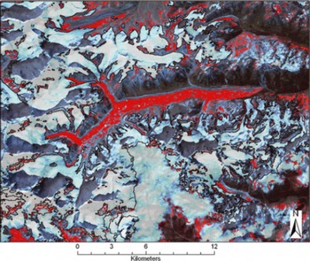
Fig. 6. Results of the debris-covered mapping algorithm using a decision tree for the Sikkim area, Indian Himalaya, based on an ASTER scene from November 2001. Pixels classified as potentially debris-covered are shown in red; clean glacier outlines are shown in black [7].
Currently, there is no single best algorithm for debris-cover mapping that can be applied to large regions without some manual corrections of the resulting outlines. The various methods for mapping debris-covered glaciers have not yet been compared and a superior method has thus not yet emerged. The basic consideration for applying a semiautomated method over fully manual correction is the required workload, which varies by region with respect to characteristics and number of the debris-covered glaciers, DEM availability and the complexity of the method. For example, complicated algorithms such as neural networks or Fuzzy C Mean clustering classifications may provide more accurate results, especially for various types of debris cover (Reference Berthier, Arnaud, Kumar, Ahmad, Wagnon and ChevallierBishop and others 1999), but the long processing time may limit their applicability over large regions.
Remaining challenges in debris-cover mapping relate to accurate identification of the glacier terminus, the separation from stagnant glacier parts and, in some areas, the lack of a high-resolution DEM needed to apply the specified algorithms. Stereo viewing of the original satellite bands, which strongly enhances visual perception, may be helpful in interpreting subtle morphological details (personal communication from V. Aizen, 2008). However, one of the greatest remaining challenges is the validation of the existing debris-cover algorithms. Possibilities for validation include use of velocity maps derived from feature tracking, field campaigns using radar techniques or drilling, georeferenced ground photos or calculation of thickness changes from DEM differencing. Given that it may be difficult to locate the boundary of a debris-covered glacier even in the field (e.g. Reference Hall, Riggs and SalomonsonHaeberli and Epifani, 1986), the uncertainty in mapping debris-covered glaciers from satellite data remains high no matter what technique is used and this should be acknowledged in any glacier inventory and analysis derived from it.
Technical recommendations
1. In choosing an algorithm for debris-cover mapping, the analyst should consider the software availability, the type of image being analyzed and the type of terrain.
2. Given the complexity of the debris-cover mapping methods, the algorithms presented above may be used as a guide or a starting point for manual delineation.
3. Over large regions, manual delineation of debris-covered glacier ice is very time-consuming (about 5 min per glacier) and the analyst might consider relying on automated algorithms while acknowledging the errors associated with these algorithms.
4. Visual identification of debris-covered parts may be strongly enhanced by utilizing stereo-viewing techniques on the original images (e.g. using ASTER bands 3N and 3B).
5. Surface slope and vegetation maps may work well in most cases. If thermokarst features are present (hummocky surface), the analyst should either use a different method, or try to first fill the holes in the DEM (sinkholes) using various available interpolating methods.
6. Terrain curvature can work well for delineating debris-covered regions when marked moraines are visible on the DEM.
7. Using the highest-resolution DEM available is not always advisable because of the noise in the data and the additional features that become visible, so terrain smoothing may be useful in some cases before applying the algorithms.
8. ‘Special cases’ mentioned above should be identified and treated specifically, possibly by using manual delineation.
9. Visual inspection of the derived debris-cover maps and final editing are always required.
Ice-divide mapping
The purpose of ice-divide mapping is to identify glacier entities in an objective and consistent manner, for hydrologic applications (e.g. glacier runoff) and glaciological applications (e.g. change detection). Generally, ice divides may be identified faster using semi-automated algorithms (hydrologic modeling tools) than by visual interpretation, but a DEM is required in the former case. Three basic considerations need to be addressed: (1) where to place the divide; (2) how to delineate it automatically; and (3) how to match ice divides from recent imagery with formerly used ice divides derived from topographic maps. Also, the type of glacier must be considered (e.g. ice field, ice cap, outlet glacier, mountain/valley glacier and glacieret) before a separation is made. Ice fields consist of a central ice mass (with nunataks) from which several ‘outlet glaciers’ originate. An ice cap is a dome-shaped mass of ice, not divided by topography, which may also have ‘outlet glaciers’, and is most commonly found on top of volcanoes or in Arctic regions (Reference PaulMüller and others, 1977). For both types it can be very challenging to find or assign divides in the accumulation area and thus the analyst may opt to treat the entire system as one entity in the beginning. This might apply, for example, for the rather complex ice-cap system on Baffin Island, which is depicted in Figure 7. Valley or mountain glaciers are confined to a valley and may have tributaries. These glacier types usually have easily identifiable upper divides due to the presence of rock outcrops (see Fig. 4), but determining whether tributaries should be included may be challenging, depending on whether these tributaries contribute substantially to the mass of the glacier. Several methods for delineating ice divides for the above four types were illustrated in oral presentations at the workshop and are summarized below.
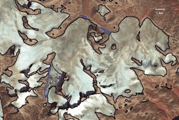
Fig. 7. A system of ice caps with complex topology on Baffin Island, Canada, as seen on a Landsat ETM+ satellite image from August 2002 (bands 4, 3, 2 as RGB). Black lines indicate automatically generated glacier outlines; blue lines enclose (partly ice-covered) lakes and have been deleted manually.
Challenges
Algorithms
A first starting point for ice-divide mapping is a flow-direction and/or watershed grid derived from the DEM. This can be used in many cases to digitize the ice divides accurately (Reference Paul and Kääb.Paul and Andreassen, 2009) but is rather time-consuming. Other automated methods were also presented at the workshop. One study [4] described an approach for ice-divide delineation which consists of: (1) generating a buffer around the glacier; (2) calculating basins based on a DEM; and (3) removing all basins without a glacier (Fig. 8). An algorithm developed by Reference Müller, Caflisch and MüllerManley (2008) was illustrated for the Afghanistan and Cordillera Blanca glaciers, respectively [1, 6]. Manley’s algorithm consists of creating ‘contiguous ice’ polygons, identifying ice divides for them using DEM analysis, then ‘cutting’ the contiguous ice polygons along the ice divides. The steps are: (1) calculating the median elevation for each ice mass; (2) isolating the ‘toes’ of the ice masses, where each toe is identified by ice gridcells with elevations lower than the median elevation for the ice mass; (3) using the toes as ‘pour points’ (starting points for watershed analysis) to identify separate glacier basins (watersheds); (4) identifying complex ice masses (those with more than one toe, and only those larger than a variable area cut-off, depending on the number of toes per ice mass); (5) isolating basin areas within the complex ice masses (‘complex basins’); (6) converting the complex basins to polygons; and (7) overlaying the basin polygons on the ice polygons. The result of the algorithm depends on the choice of less-than-median-elevation for toes that act as ‘pour points’ for glacier basins. ‘Pour points’ can be digitized manually or derived automatically (Reference Singh and BengtssonSchiefer and others, 2008).
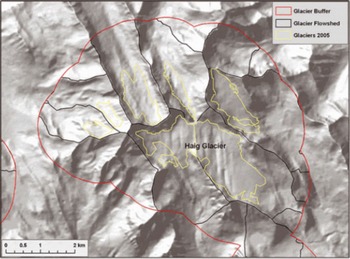
Fig. 8. Schematic illustration of the ice-divide mapping algorithm using DEM analysis in Western Canada. The background shows a shaded relief from the used TRIM DEM [4].
The methods presented above rely on the availability of an appropriate DEM, which is not always available for some glacierized regions. Furthermore, it must be mentioned that DEMs based on optical imagery often have inaccuracies in the accumulation zones of the glaciers (where the ice divides are situated) due to low or almost no contrast on the snow-covered areas (Reference VanLooy and ForsterToutin, 2008; Svoboda and Reference Paul and Kääb.Paul, 2009). In the absence of a DEM, illumination differences and glaciological knowledge about glacier flow can be applied for a first estimation of the ice-divide position (cf. Reference Paul, Huggel and KääbPaul and Kääb, 2005). Ice divides derived in this way can be revised later in the digital database when DEM information becomes available.
Challenges
The types of difficulties faced in applying the ice-divide algorithms depend on whether the ice bodies are ice caps or ice fields, complex topologies or compound glacier types. Such cases need to be addressed separately in most cases. It is important to acknowledge that the choice of an ice-divide mapping method depends on the intended application. Consistency with ice divides from various years is desirable for change analysis studies, such as area changes, to minimize errors. However, it is necessary to consider that ice divides may change and glaciers may disintegrate, requiring the delineation of new ice divides [4]. The analyst can start with the largest possible (e.g. Little Ice Age) extent, which can be used subsequently to track the changes of the entire system
Technical recommendations
The choice of an ice-divide algorithm requires a DEM for watershed modeling, and glacier outlines derived from topographic maps or satellite imagery. The following recommendations are based largely on a case study in Baffin Island (Reference Paul, Huggel and KääbPaul and Kääb, 2005) as well as on other participants’ expertise compiled during the working session on ice-divide mapping:
To a large extent, choosing a location for the ice divide depends on the purpose of the glacier inventory and the glacier type (e.g. ice caps of varying complexity). Four scenarios were identified:
1. When a former glacier inventory already exists and a comparison with these former glacier extents is envisaged, ice divides should be placed at the same locations as in the former inventory. When the old ice divides are not available digitally but have to be digitized from printed (sketch) maps, a larger error must be considered (which might even be larger than the real area change).
2. If the purpose of glacier mapping is a hydrologic one (e.g. to calculate specific runoff from a catchment), the glaciers should be divided in a hydrologic way. Given an accurate orthorectification of the satellite data, readily available digitized catchments should be used. To some extent it might be possible to use major hydrologic divides instead of those related to a lower stream order.
3. When no former inventory is available, glaciers should be divided in a more glaciological sense. However, principal rules of a hydrologic numbering scheme (see Reference PaulMüller and others, 1977) should also be considered. Where printed maps with point data from the WGI are available (e.g. as for Baffin Island), they should be considered as an identifier for individual entities.
4. Ice caps can be divided into distinct units when they are well defined. When they are more compact or the units are not clear, they should not be subdivided (see Fig. 7).
The algorithms to be applied for digitizing ice divides mostly depend on the availability of a (reliable) DEM. Two scenarios were identified:
1. When no DEM is available, a best guess of the location should be made based on illumination differences and glaciological knowledge about glacier flow. Uncertain divides in the accumulation region can be indicated by straight lines and a lower positional accuracy in the metadata table for the respective line segment.
2. When a DEM is available, the first step is the calculation of a flow direction grid that allows delineating divides manually. A second step is the calculation of watersheds or upslope area from given pour points. A third step is the application of the above-mentioned automated methods.
DEM generation
DEMs are used by glaciologists to derive glacier parameters such as length (using flow direction functions), terminus elevation, median elevation, hypsometric information and glacier flow patterns. When combined with glacier outlines, DEMs are also useful for defining ice divides from flow direction grids and watershed analysis in a semi-automated fashion [4, 5], and for orthorectification of satellite imagery. DEMs from different time-steps may be used to determine changes in glacier surface elevation at decadal scales (e.g. Reference Svoboda and PaulSurazakov and Aizen, 2006; Reference MeierLarsen and others, 2007; Reference RahmstorfRacoviteanu and others, 2007; Reference Sidjak and WheateSchiefer and others, 2007; Reference Paul, Hendriks, Pellika and ReesPaul and Haeberli, 2008). While DEM accuracy is a key issue for glaciological applications, there is no consensus within the glaciological community regarding the best software package and methodology for generating DEMs from satellite imagery. This section describes the most commonly available commercial DEM-generation software packages that are designed to work with satellite-image stereo pairs, and attempts to describe the strengths and weaknesses of each. The goal here is not necessarily to advise on which package works best under various conditions, or even to provide relative error assessments, but only to provide some characteristics of the packages and to list some implications for glacier studies. Most of these points were summarized in one presentation in the GLIMS workshop [8] and were discussed in the DEM working group.
Commercial software currently available for DEM generation from satellite-image stereo pairs includes: Geomatica from PCI Geomatics, ENVI from ITT Visual Information Solutions, Leica Photogrammetric Suite (LPS) from ERDAS, Silcast from Sensor Information Laboratory Corp., Desktop Mapping System (DMS) from R-WEL and Photomod from Racurs. Recent efforts have been undertaken to validate DEMs derived from ASTER (Reference KääbKääb, 2002; Reference ToutinToutin, 2002; Reference KääbHirano and others, 2003; Reference Bolch and G.M.Bolch, 2004; Reference Dyurgerov and MeierEckert and others, 2005; Reference Fujisada, Bailey, Kelly, Hara and AbramsFujisada and others, 2005; Racoviteanu and others, 2007), SPOT (Reference LemkeKrupnik, 2000; Reference Berthier, Arnaud, Vincent and RémyBerthier and others, 2007) and SRTM (Reference Sun, Ranson, Kharuk and KovacsSun and others, 2003; Reference BerthierBerthier and others, 2006; Reference Carabajal and HardingCarabajal and Harding, 2006). Other studies focused on comparing the SRTM DEMs with ASTER DEMs (Reference Fujita, Suzuki, Nuimura and SakaiFujita and others, 2008; Reference KääbHayakawa and others, 2008). For a detailed review of the methods, algorithms and available commercial software to extract elevation from ASTER satellite imagery, and its various applications in geoscientific applications, the reader is directed to a recent review article by Reference VanLooy and ForsterToutin (2008).
There is a need for further accuracy assessment in the specific context of glacier studies. One study presented in the GLIMS workshop [8] processed three ASTER scenes containing glaciers in different regions of the world (Cordillera Blanca in Peru, Lahul-Spiti in western Himalaya, and the Antarctic Peninsula) using four different packages: PCI, ENVI, Silcast and LPS. The resulting DEMs were compared and the results and experiences in using these packages are summarized in Table 2. The packages vary widely in sophistication and ease of use, with LPS requiring the most training before all its features can be properly utilized and Silcast requiring nothing more than an input file. Although LPS offers the most options for optimizing the DEM generation process, it does not uniformly produce the best DEM. We believe that this is in part due to the fact that in the version we were using (9.2) the pre-processing routines for radiometric corrections were not working properly. In summary, there is no one package that performs best under all circumstances – each has its strengths and weaknesses. The trade-offs include performance, cost, control and ease of use.
Table 2. Summary of features and functionality of four software packages capable of generating DEMs from ASTER stereo pairs [8]. Version of Silcast used by the LP DAAC was not available; products ordered 3 April 2008. GcPs: ground control points; TPs: tie points
Challenges
Challenges in DEM extraction from optical satellite imagery are manifold and include among others: lack of ground control due to logistical, cultural and/or political issues; lack of contrast over accumulation areas of the glacier or in regions of shadow, exacerbated by suboptimal instrument gains; the presence of clouds on the satellite scene being analyzed; and obscuration of terrain due to the looking direction of the stereo sensor. Users must be cognizant of errors inherent in DEMs derived from remote-sensing imagery, such as elevation and slope biases (Reference Kaser, Cogley, Dyurgerov, Meier and OhmuraKääb and others, 2003; Reference BerthierBerthier and others, 2006; Racoviteanu and others, 2007; Reference GeorgesFujita and others, 2008; Reference Paul, Hendriks, Pellika and ReesPaul, 2008).
For some glaciological applications, a one-time modernera global DEM of adequate spatial resolution and well-characterized errors would be desirable. As mentioned earlier, the DEM derived from the SRTM has found application within the community, although the biases, voids and the 3 arcsec resolution limit its utility. The Silcast software has been used to produce a GDEM at 1 arcsec resolution from about 30 000 ASTER scenes. The product is due for completion mid-2009 (http://www.ersdac.or.jp/GDEM/E/). A recent study focused on comparing a prerelease version of the GDEM and the SRTM-3 (Reference KääbHayakawa and others, 2008). A validation summary of the ASTER GDEM produced by the Ministry of Economy, Trade and Industry (METI), Japan, and NASA was recently released and is available from https://lpdaac.usgs.gov. This study concludes that the overall accuracy of the global ASTER DEM can be taken to be approximately 20m at 95% confidence interval. While the accuracy of carefully generated DEMs from satellite data might be higher than the near-global products (SRTM, GDEM), the latter might be well suited to derive detailed glacier inventory data on a global scale. Further studies comparing the different DEM sources and software packages quantitatively will be performed in the future.
Technical recommendations
Quality control of the DEMs is essential before they are applied for glacier studies. Acceptable errors depend on the intended application. These include, in order of increasing accuracy requirement: extracting topographic information (slope/aspect) which does not change rapidly, orthorectification of satellite imagery, hypsometry, extracting glacier parameters (e.g. minimum/mean/maximum elevations), and geodetic mass balance (from DEM differencing). DEMs can be derived from topographic maps by interpolating either points or contour lines digitized from these maps. The accuracy of the resulting DEM is largely dependent on the type of terrain and the interpolation method used (Racoviteanu and others, 2007; Reference KääbKääb, 2008). DEMs from satellite imagery are constructed by stereo-correlation procedures with the above mentioned specialized software packages. Below is a summary of steps that may be used to minimize DEM errors and to conduct quality control on DEMs for both topographic maps and satellite imagery.
1. In choosing a satellite scene for DEM generation, the following should be considered:
the quality of source imagery such as channel gains (high gains provides detail in shadow regions, but may result in saturation over the accumulation area); the degree of cloudiness, their possible elevation and maybe a predefined cloud mask;
the date of acquisition: for area change detection and mass-balance applications, the satellite scene should be acquired at the end of the ablation season with minimal seasonal snow;
the choice of spatial resolution influences the output DEM. The cell size should be chosen according to terrain characteristics (higher resolution for rugged terrain, lower resolution for smooth terrain).
2. Ground-control points (GCPs) acquired in the field for DEM generation and/or evaluation should be spread across the scene, away from steep slopes and have similar slope/aspect to the glacier. The placement of the antenna must be included in GCPs from the field as this can induce vertical errors of a few meters.
3. Methods of assessing the accuracy of DEMs derived from either map or satellite imagery include:
examining the root-mean-square error in the vertical coordinate (RMSEz) with respect to GCPs;
identifying artefacts such as blunders and outliers, using hillshades, profile curvature, elevation histograms, DEMs with coarser cell size and slope maps;
performing a trend assessment on the DEM to detect biases;
comparing transects from the DEM with field data;
specifically for DEMs constructed from topographic maps using interpolation, spot elevation from the DEMs can be compared with points extracted from the original contours to determine the accuracy of each interpolation method;
for DEMs created from satellite imagery, software reports such as score channel and error maps;
for a reliable DEM, the orthorectified stereo bands (e.g. ASTER 3N and 3B) should match exactly. DEM errors that may occur due to mismatching can be calculated by dividing the shift through the stereo ratio of the sensor (e.g. 0.6 for ASTER);
when a DEM is created from mosaicking several scenes together, examining discontinuities at mosaic seams will provide information on the accuracy of the orthorectification process and DEM extraction.
4. Some suggestions for improving the quality of the resulting DEMs include:
pre-processing (selection of cloud-free satellite scenes with good contrast over snow and ice), stretching, sharpening and filtering;
ensuring a good distribution of GCPs and avoiding questionable ones;
downsampling of the epipolar image pairs;
post-processing/editing such as hole filling from DEMs with coarser resolution, interpolation, and terrain smoothing.
Change detection
Multitemporal analysis is used to detect changes in various glacier parameters such as area, length, elevation, proglacial lakes, debris cover and internal rock. Important issues relating to change detection include accurate and consistent orthorectification, flowline digitization, the date of acquisition of the data used for DEM generation, and their spatial resolution. Regarding the latter, it must be emphasized that medium-resolution satellite DEMs (ASTER/SRTM) are more useful for assessing changes in glacier surface elevation for large glaciers and on decadal timescales. High-resolution DEMs (e.g. derived from aerial photogrammetry or lidar) can also be used for small glaciers (area < 1km2) and/or for shorter timescales (annual changes). Further details on the detection of glacier area changes can also be found in Reference Paul, Hendriks, Pellika and ReesPaul and Hendriks (2009).
Examples of deriving glacier area changes from multi-temporal analysis of satellite images in the context of the GLIMS initiative are numerous. A small selection of such studies, conducted by some of the GLIMS researchers, include Reference BarryBayr and others (1994), Reference KargelKääb and others (2002), Reference Paul, Kääb, Maisch, Kellenberger and HaeberliPaul and others (2002,2004b, Reference Racoviteanu, Arnaud, Williams and Ordoñez2007), Reference Hayakawa, Oguchi and LinHall and others (2003), Reference KulkarniKhromova and others (2003, Reference Kulkarni2006), Reference Bolch, Kamp, Kaufmann and SulzerBolch and Kamp (2006), Reference Bolch, Buchroithner, Kunert and KampBolch (2007) and Racoviteanu and others (2008a). The approach of deriving changes in glacier surface elevations from multiple DEMs was used in several studies on the basis of historical topographic maps and DEMs derived from SPOT imagery (e.g. Reference Bayr, Hall and KovalickBerthier and others, 2004,Reference Berthier, Arnaud, Vincent and Rémy2007), SRTM (Reference RöhlRignot and others, 2003; Reference Svoboda and PaulSurazakov and Aizen, 2006; Reference MeierLarsen and others, 2007; Racoviteanu and others, 2007; Reference Sidjak and WheateSchiefer and others, 2007; Paul and Haeberli, 2008), ASTER (Reference RottRivera and Casassa, 1999; Reference KääbKääb, 2008) and laser altimetry (Reference Aniya, Sato, Naruse, Skvarca and CasassaArendt and others, 2002). A combination of optical imagery (SPOT HRV, Landsat TM and ASTER) and synthetic aperture radar (SAR) (European Remote-sensing Satellite (ERS), RADARSAT) data, as well as high-resolution DEMs derived from the Panchromatic Remote-sensing Instrument for Stereo Mapping aboard the Japanese Advanced Land Observing Satellite (ALOS PRISM) launched in 2006 and Corona (Reference PaulNarama and others, 2007; Reference Bolch, Buchroithner, Pieczonka and KunertBolch and others, 2008), provide potential for thickness change estimations over small regions, but they are not particularly useful for achieving global DEM coverage.
Challenges
Various presentations [1, 4, 6] addressed challenges in glacier change detection studies and comparison with old topographic data, posed by inconsistencies in the various data sources and processing steps. Such challenges include: geometric changes in glacier topography such as rock outcrops, splitting or disintegration of glaciers; and inconsistencies arising from comparing data from various sources, for example satellite-derived data vs data derived from topographic maps, or comparison with the point data as stored in the WGI. The largest sources of error in the estimates of area changes may come from errors in the baseline data sources, mostly in the case of old data from topographic maps. For example, two studies conducted in the Cordillera Blanca (Reference Gregory and OerlemansGeorges, 2004; Racoviteanu and others, 2008a) point out that the glacierized area in the 1970 baseline inventory was overestimated by as much as 10% due to seasonal snow, thus resulting in a larger estimated area change from 1970 to the present. Racoviteanu and others (2008a) point to apparent growth in glacier areas of as much as 100% due to digitizing errors in the baseline glacier inventory of the Cordillera Blanca, mostly in debris-covered areas. Other challenges for area change detection are posed by use of poor-quality satellite images, the presence of seasonal snow in the accumulation region of glaciers and the presence of debris cover on the glacier surface. Challenges in vertical change detection using multiple DEMs could be related to inconsistencies in horizontal/ vertical datums in the various elevation datasets being compared or penetration of the radar beam into dry snow for interferometric SAR (InSAR)-derived DEMs (Reference FarrFarr and others, 2007). For example, Racoviteanu and others (2007) report an apparent glacier thickening at high elevations of Nevado Coropuna, Peru, due to known errors in the baseline topographic map. Such errors are common when the topographic map was derived from aerial photography with low contrast in the accumulation areas, and pose a major problem in elevation change studies. To minimize such inconsistencies, a few recommendations are listed below.
Recommendations
For calculation of glacier area changes between two points in time, the following issues should be considered:
1. When possible, area change calculations should be derived from similar datasets (e.g. same type of satellite imagery).
2. The change should be calculated by subtracting the obtained total sizes in each analyzed year and not by digitally subtracting the glacier maps.
3. To minimize inconsistencies, the use of the same type of data by the same surveyor and the same analysis methods is recommended.
4. There should be consistency in upper glacier boundaries, internal rocks, debris cover and snow cover among various inventories used for comparison. If inconsistencies exist in parts of the dataset, selecting a subsample of the glacier dataset for detailed change analysis is recommended (Racoviteanu and others, 2008a).
5. If glacier outlines from different sources are compared (e.g. one set of outlines derived from older topographic maps and the other from satellite imagery), special care must be taken that exactly the same entities are compared. In such cases and for analysis purposes, drainage divides should be kept constant for both datasets, thus ignoring any changes in the position of the ice divides [4] (Reference Racoviteanu, Arnaud, Williams and OrdoñezPaul and others, 2007; Racoviteanu and others, 2008a; Reference Paul and Kääb.Paul and Andreassen, 2009).
In assessing changes in elevation from multiple DEMs, the following points may be considered:
1. Any physical changes on the glacier surface over the period of evaluation (e.g. snow amount, lake formation) should be considered.
2. Change detection analysis should be avoided in regions where DEM values are interpolated.
3. It should be taken into account that DEMs from optical stereo are often inaccurate in accumulation areas (e.g. Reference Sidjak and WheateSchiefer and others, 2007; Reference Wessels, Kargel and KiefferVanLooy and Forster, 2008).
4. The distribution of vertical errors between two DEMs with respect to elevation and slope should be quantified.
5. Elevation differences should be computed on non-glacierized terrain vs glacierized terrain and care should be taken that they are as flat as possible to avoid resampling artefacts (Reference Paul, Kääb, Maisch, Kellenberger and HaeberliPaul, 2008).
6. If difference maps look like hillshade maps, this indicates a geolocation registration error (shift).
7. When using spaceborne altimetry data (ICESat) or InSAR (ERS, SRTM) in evaluating DEM accuracy, errors arising from signal saturation and beam penetration should be considered.
8. Changes in topographic parameters such as minimum or mean glacier elevation through time are difficult to quantify if there were strong changes in glacier geometry, such as separation of tributaries or disintegration of ice masses, as noted in various studies (Reference Rabus, Eineder, Roth and BamlerPaul and others, 2004a; Reference Manley, Williams and FerrignoKulkarni and others, 2007; Racoviteanu and others, 2008a). The related rules and recommendations for such calculations have yet to be defined.
Errors in Remote Sensing of Glaciers
Given that the assessments of glacier area are sensitive to the quality of the data used to derive them, the issue of uncertainty and its propagation in glacier delineation based on remote sensing deserves proper consideration. So far, only a few glaciological studies (Reference Hirano, Welch and LangHall and others, 2003; Reference Rignot, Rivera and CasassaRaup and others 2007b) have provided careful evaluations of uncertainty in glacier mapping using ground data. At the core of the problem is the lack of systematic ground-control data (such as DGPS measurements) to evaluate errors in the derived glacier outlines. In most cases, all glacier outlines are validated and corrected against a ground truth (e.g. visual comparison with the satellite image). Since an independent ground truth is often not available, standard measures of accuracy no longer apply (see Reference Takeuchi, Kayastha and NakawoSvoboda and Paul, 2009). However, it is possible to differentiate between certain types of error, and for some of them accuracy measures are available.
In remote sensing of glaciers, the main sources of uncertainty may arise from: (1) positional errors (geocoding, GCPs); (2) classification errors (misidentified features); (3) processing errors (e.g. from digitization, coordinate precision, attribute data, ‘sliver’ polygons resulting from overlay operations); and (4) conceptual errors (e.g. glacier definition issues such as ice divides, perennial snowfields, minimum size, and fragmentation). While errors of type (1), (2) and (3) are generally small and can be calculated by standard statistical methods (Reference CongaltonCongalton, 1991; Reference Zhang and GoodchildZhang and Goodchild, 2002), conceptual errors can be quite large but difficult to quantify. In order to identify the latter, several so-called GLIMS analysis comparison experiments (GLACE) have been performed (Reference Rignot, Rivera and CasassaRaup and others, 2007b). They helped to design the guidelines of the GLIMS Analysis Tutorial, which could be seen as a large step forward regarding the consistency of the GLIMS database entries. Presently, it is possible to store errors of type (1) and (3) for each glacier in the database. Type (2) and (4) errors currently can be identified (at least partly) by visual inspection of the outlines using 3-D digital overlays or stereo viewing.
Conclusions and General Recommendations
The GLIMS workshop held in Boulder, CO, USA, in June 2008 focused on the current state of glacier monitoring from satellite imagery in the context of the GLIMS initiative. Presentations and working groups addressed algorithms and challenges for glacier delineation and DEM generation and analysis. The workshop participants also aimed at establishing protocols and providing a set of tools and algorithms for glacier delineation and DEM generation, which can be used by GLIMS regional centers. As a result of the workshop, the GLIMS algorithm page hosted at http://glims.org will be updated to contain code, scripts and processing steps that will be shared within the GLIMS community.
Currently, fully automated inventorying of individual glaciers from threshold ratio satellite images is hampered by challenges encountered with mapping of debris-covered glaciers, separation of seasonal snow from perennial snow and glacier ice, and finding the correct location of ice divides [9]. Topographic shadowing effects, clouds and water bodies can be corrected by visual interpretation and manual editing. Many workshop presentations demonstrated that the use of digital terrain information in a GIS greatly facilitates automated procedures of image analysis, data processing and modeling/interpretation of newly available information. General recommendations with respect to glacier delineation and analysis in a remote-sensing and GIS environment are given below:
1. Refer to published tutorials and algorithms, such as the GLIMS Analysis Tutorial.
2. Compile and make use of additional material that facilitates the glaciological interpretation, such as oblique photos, topographic maps, published glacier inventory data in digital (coordinates) or analog (books) form, and ground photos.
3. Use the freely available and already orthorectified scenes from Landsat TM/ETM+ (USGS, http://landsat.usgs.gov)to check for geolocation errors.
4. Start with the most simple image classification method and test more advanced methods when the required input (e.g. a DEM) is available.
5. Select thresholds for band ratios that minimize the workload needed for post-processing (i.e. manual editing).
6. Thoroughly document the applied techniques (e.g. thresholds, filters, and manual interpretation).
7. Keep one original image classification result and apply any corrections (e.g. debris delineation and water body separation) on a copy.
8. Apply necessary manual corrections to remove regions that should not be taken into account for glacier area (e.g. seasonal snow and proglacial lakes).
9. Change assessments should be carried out at decadal scales between (dated) trimlines of the Little Ice Age (~1850s) and ~2000, with respect to the global baseline inventory.
10.Metadata are essential to face the challenges of using different mapping techniques (e.g. maps vs aerial photos vs satellite images).
Future work
Current efforts within the GLIMS initiative focus on further systematizing the process of extracting glacier boundaries from satellite imagery. We expect that these efforts will lead to a more consistent and higher-quality database of glaciers that can be used for many scientific purposes. We are additionally focusing on integrating the GLIMS Glacier Database with other global glacier databases, such as the WGI. Challenges in achieving this task are posed by: difficulty in matching up corresponding records due to poor geolocation in some cases, differences in snow–firn–ice differentiation among the different databases, disintegration and disappearance of glaciers, missing meta-information, different methodologies and data formats between WGI and GLIMS and other databases, and limited capacities of monitoring services. To minimize inconsistencies in various databases in the future and to aid the process of integration of the various databases, future steps should focus on: defining key regions that are relevant for climate change, sea-level rise, hydrological questions and natural hazards; providing guidelines and algorithms for calculation of glacier parameters from digital sources; conducting detailed inventories at decadal scale in these regions; linking annual in situ measurements with decadal remote-sensing data for change assessments; providing a better definition of priorities and workflows for the different datasets; and improving the coordination of efforts between the key players such as the WGMS, NSIDC, GLIMS, international organizations and the wider scientific community
Acknowledgements
The GLIMS team at NSIDC is supported by NASA awards NNG04GF51A and NNG04GM09G. A. Racoviteanu’s research is supported by a US National Science Foundation (NSF) doctoral dissertation improvement award (NSF DDRI award BCS 0728075) and a NASA Earth System Science Fellowship (NNX06AF66H). The work of F. Paul has been performed within the framework of the European Space Agency project GlobGlacier (21088/07/I-EC). We thank V. Aizen and T. Bolch for their constructive comments. We are grateful to all the workshop participants for their feedback, discussion and ongoing input to the GLIMS project.


