


Introduction
Ice is commonly regarded as an extremely slippery material because it has a coefficient of friction µ an order of magnitude lower than other crystalline solids under conditions at which most people interact with it. Historically the high-resolution microscopic observation of ice surfaces has been problematic, so the processes related to ice friction have been determined using an analytical approach (Reference Bowden and HughesBowden and Hughes, 1939; Reference Bowden and TaborBowden and Tabor, 1950) or have been inferred from the relationship between friction force and a series of parameters used in tribological experiments (Reference Barnes, Tabor and WalkerBarnes and others, 1971; Reference Evans, Nye and CheesemanEvans and others, 1976; Reference Kennedy, Schulson and JonesKennedy and others, 2000). More recently, plane-light microscopy of wear surfaces has been used to characterize ice friction processes (Reference Montagnat and SchulsonMontagnat and Schulson, 2003). Here we present a method for the observation of ice wear surfaces using low-temperature scanning electron microscopy (LT-SEM), which allows the interpretation of friction processes based on the morphology of the ice debris.
Friction on ice has been the subject of scientific enquiry for more than 100 years (Reference JolyJoly, 1887; Reference ReynoldsReynolds, 1900) and it has long been recognized that µ for ice is strongly dependent on the temperature T of the ice–slider system and the sliding velocity v (Reference Bowden and HughesBowden and Hughes, 1939). At velocity greater than ~0.01 ms−1 and temperature greater than −10ºC, frictional heating is sufficiently high to melt the ice surface and provide a lubricating film of liquid water (Reference Bowden and HughesBowden and Hughes, 1939; Reference Bowden and TaborBowden and Tabor, 1950; Reference Evans, Nye and CheesemanEvans and others, 1976). for a given load, the frictional heating and the thickness of the fluid film increase with velocity, resulting in a reduction of friction as speed increases. At a velocity less than ~0.01 ms−1, frictional heating is not sufficiently high to lubricate the ice–slider interface, and frictional sliding proceeds via the deformation of asperities and surface fractures (Reference Barnes, Tabor and WalkerBarnes and others, 1971; Reference TusimaTusima, 1977; Reference RistRist, 1997; Reference Montagnat and SchulsonMontagnat and Schulson, 2003). Thus at low sliding velocity, µ is controlled by the creep rate of ice (Reference Barnes, Tabor and WalkerBarnes and others, 1971), adhesion by sintering leading to asperity growth (Reference TusimaTusima, 1977; Reference Maeno and ArakawaMaeno and Arakawa, 2004), or a combination of both processes (Reference Kennedy, Schulson and JonesKennedy and others, 2000).
The presence and thickness of a lubricating fluid is also dependent on the thermal properties of the slider. Frictional heat generated at the sliding interface is partitioned between the ice and slider depending on their relative thermal conductivity and heat capacity. Lubricating fluid is produced when the heat conducted into the ice is sufficiently high to overcome the latent heat of fusion and raise the temperature to the melting point of ice. for sliding at constant velocity a greater thickness of fluid is produced and µ is reduced as the temperature of the ice–slider system approaches the melting point of ice (Reference Bowden and TaborBowden and Tabor, 1950).
Observation of wear surface morphologies can give an insight into the frictional processes that produced them. The relationships between temperature, velocity and frictional processes are examined here by combining wear surface observation using LT-SEM with ice friction experiments and the development of an ice wear map. Wear maps for a variety of counter-facing materials have been used to determine how sliding occurs when different conditions are encountered (Reference Lim and AshbyLim and Ashby, 1987; Reference LimLim, 1998). Friction experiments were performed over a temperature range from −27 to −0.5ºC and velocity range from 0.008 to 0.37 ms−1 and the results contoured to construct an empirical µ-v-T wear map. The kinetic friction of ice in this velocity–temperature range is of particular interest to engineers designing structures for ice-prone regions and winter sports equipment. LT-SEM observations from different regions within the µ-v-T wear map are presented here and used to identify diagnostic wear and debris features. The morphology of wear and debris features is used to identify friction processes acting at different temperatures and velocities.
Experimental Methodology
Sample preparation
Ice hemispheres with flat sides attached to aluminium stubs were used in all tribology experiments and LT-SEM observations. Ice samples were produced by placing droplets of deionized water on 10 mm diameter aluminium sample stubs with a syringe at temperatures between −27 and −22°C. The droplets were placed within a 7 mm diameter, 1 mm deep recess within the stub and allowed to freeze. Surface tension and expansion of water during the phase transition from liquid to solid produced the hemispherical shape. The depression in the stub had a bevelled edge that locked the sample in place during experimentation and LT-SEM observation (Fig. 1a).

Fig. 1. (a) Aluminium sample stub with bevelled edge used to hold ice hemispheres in friction experiments and LT-SEM observations. (b) Dovetail with brass cap that covers aluminium stub and ice samples and prevents alteration by frost from atmospheric water. (c) Geometry of wear surface and debris relative to transport direction.
The substrate used in all tribology experiments presented here was a 1 m long, 0.1 m wide, 2 mm thick steel sheet. The steel sheet was dry-polished using an 800 grit silicon carbide paper in a circular motion, and then scored with a coarse sheet of 60 grit silicon carbide paper to produce a consistent surface roughness. The steel sheet was then cleaned with ethanol until all traces of metallic debris were removed. The sheet was clamped to the linear tribometer and placed into a chest freezer overnight to reduce its temperature to −27°C. Before each friction experiment the steel sheet was wiped with long-fibre tissue to remove surface frost formed from atmospheric water vapour. A shorter (0.2 × 0.05 × 0.002 m) steel rail was prepared in an identical fashion for wear surface preparation in the LT-SEM laboratory.
Linear tribology
A metre-length linear reciprocating tribometer was developed and used to determine the coefficient of friction between ice hemispheres and the steel rail over a temperature range from −27 to −0.5°C and a velocity range from 0.008 to 0.37 ms−1. The tribometer consists of an aluminium carriage that travels on a rail system that confines it to linear motion (Fig. 2). Extending perpendicular from the carriage is a rectangular brass arm that is connected to a load of known mass that bears on a sample holder containing the ice hemisphere. Loads of 2.10 and 4.20 N were used during experiments. The carriage was towed using a variable voltage electric motor. Mechanical vibration was minimized by isolating the electric motor and using a cable to tow the carriage. A counterweight system was used to reciprocate the tribometer.

Fig. 2. Linear reciprocating tribometer in (a) plan view, and (b) side view.
The brass arm was engineered to allow flexure parallel to the direction of motion and to minimize horizontal axial rotation perpendicular to the motion. A pair of strain gauges was placed on either side of the arm at the point of maximum flexure to measure the deflection of the arm caused by frictional force acting between the ice sample and substrate (Fig. 2). The strain gauges were connected via a full Wheatstone bridge to two ‘passive’ strain gauges placed on a second brass plate on top of the carriage, which was fixed at one point. This arrangement eliminates the effect of thermal expansion, as all four strain gauges expand with temperature at the same rate. A 5 V direct current was placed across the bridge, and the difference in voltage at the centre of the active gauges compared to that at the centre of the passive gauges was used to determine the flexure of the brass arm. The tribometer was calibrated before and after each experimental run by attaching a spring balance to the sample holder and relating forces to the voltage output. A typical output signal is shown in Figure 3.

Fig. 3. Typical force output from linear reciprocating tribometer. This experiment was conducted at v = 0.019 m s−1, T = −25.4°C and with a load of 2.10 N. Negative force after 428 s is due to reciprocation of the tribometer.
The tribometer was placed on the floor of a chest freezer on granite blocks that acted as a heat sink. Experimental runs began at −27°C, and the power to the freezer was switched off to reduce electromagnetic interference to the output signal. The temperature of the tribometer was allowed to rise during each experimental run, and thermocouples in the steel rail and sample holder were used to record the temperature and to assess whether the sample and rail were in thermal equilibrium. The tribometer required approximately 6 hours for the temperature to rise from −27°C to 0°C, during which time 30–55 individual measurements were made. Each experiment had an experimental uncertainty in temperature of ±0.1 °C and in velocity of ±0.001 ms−1.
The analogue voltage signal from the tribometer was converted into digital data by a Pico® 212-ADC, recorded at a rate of 5 kHz and time-tagged using Pico® software. The data were imported into Matlab2, and a pattern recognition algorithm used to identify the start and finish of each experiment. The coefficient of friction was calculated as the mean ratio of the shear and normal stresses precluding the first 0.1 m of the experiment, which was the maximum distance required for the carriage to accelerate to constant velocity.
Wear surface observation
Wear surface observations were performed using a Hitachi 4700 low-temperature scanning electron microscope fitted with a Gatan Alto 2500 cryopreparation system, which uses a cold field-emission electron source. The temperature of samples must be reduced to liquid nitrogen temperature before entering the LT-SEM. This has proved problematic, as frost from atmospheric water vapour immediately covers the sample. In the case of biological samples, this frost is sublimed from the sample within the vacuum chamber of the LT-SEM, but clearly this is not appropriate with an ice sample as it would also sublime ice from the wear surface. To prevent ice contamination of the wear surface, the following procedure was adopted. Wear surfaces were prepared adjacent to the LT-SEM in a small chest freezer. The linear tribometer was used to prepare wear surfaces on ice hemispheres under a load of 4.20 N. A shorter 0.20 m steel rail was used due to space restrictions in the freezer; otherwise the sample preparation was identical to that used to produce the ice friction map. Samples were immediately removed from the tribometer’s sample holder and placed in a dovetail specimen-carrier that slides into the LT-SEM stage. The temperature of the specimen-carrier was pre-equilibrated with the temperature of the friction experiment. The dovetail is customized with a hinged brass cap that covers the ice sample (Fig. 1b). Samples were placed in the dovetail and capped with care to ensure that the cap did not come into contact with the samples’ surfaces. Sample and dovetail were then cryofixed in liquid nitrogen within the chest freezer to preserve the wear surface morphology and to prepare the sample for the LT-SEM. Any frost contamination from atmospheric water thus formed on the outside of the brass cap, and adulteration of the ice sample’s surface was dramatically reduced. The samples were immediately transferred to the vacuum chamber of the LT-SEM, and a coating of 6–8 nm of 60/40 gold/palladium alloy applied. The period of time between wear surface preparation and entry into the LT-SEM varied between 2 and 4 min. No samples cracked due to thermal contraction during the cyro-fixation process, though some samples were damaged during transportation to the LT-SEM.
Results
Ice friction map
An ice friction map was produced by plotting each of the 449 friction experiments in temperature–velocity space and contouring the coefficient-of-friction data. Data were interpolated using a mesh with 0.5°C temperature spacing and 0.02 ms−1 velocity spacing (Fig. 4). No significant variation in µ with load was found, so the map contains data for loads of 2.10 and 4.20 N. The independence of µ with respect to load is consistent with the results of previous authors (Reference TatinclauxTatinclaux, 1989; Reference Kennedy, Schulson and JonesKennedy and others, 2000). The maximum coefficient of friction was µ = 0.170 and occurred at v = 0.006 m s−1 and T = −23.1 °C. µ decreased rapidly with increasing temperature and velocity above T = −18.5°C and v = 0.05 m s−1 (Fig. 4). Contour lines below −15°C are steep, indicating strong temperature dependence at low temperature. At temperatures higher than −15°C the coefficient of friction is consistently low (<0.05) (Fig. 4). The minimum friction was µ = 0.042 and occurred both at v = 0.02 m s−1 and T = −0.5°C and at v = 0.27 m s−1 and T = −1.3°C.

Fig. 4. µ-v-T map for ice on steel. Contours of the coefficient of friction with the temperature and velocity of each friction test identified. 449 data points were contoured with loads of 2.10 and 4.20 N. Positions of samples examined with LT-SEM are identified.
Wear surfaces
Wear surfaces were examined using LT-SEM methods, and three specimens are presented here that are representative of distinctively different parts of the wear map (Fig. 4). Samples were tested on a steel rail under a load of 4.20 N. The samples exhibited different wear and debris morphologies indicative of the processes that formed them. The wear surface is defined as the area of each hemisphere that was in contact with the substrate and the debris, defined as the material from the ice sample that was transported during sliding either as liquid or as solid and often accumulated at the trailing edge of the wear surface (Fig. 1c). The ice hemispheres were composed of coarse (>200 µm), euhedral, interlocking crystals (Fig. 5). Before being worn, grain boundaries and air bubbles were visible on the surfaces of the ice samples, but they were otherwise relatively featureless (Fig. 5).

Fig. 5. An example of the surface of an ice hemisphere prior to a wear experiment. A grain boundary is visible and gives an indication of the coarse-grain nature of the ice hemispheres, and air bubbles are visible on the sample surface. Angular crystals on the surface are frost crystals that formed during cryofixation.
The wear surface on sample A was produced at high temperature (−3.4°C), low velocity (0.02 m s−1) and µ = 0.06 (Fig. 6). The relationship between the transport direction, wear surface and debris surface is shown in Figure 6a. Linear wear grooves are visible parallel to the direction of transport on the wear surface, sloping ~20º towards the lower right corner. Euhedral crystals in the background (Fig. 6a) and to the left formed on the flank of the ice hemisphere before the sample was tested. The debris appears as a large cohesive mass of ice on the trailing side of the wear surface. Running parallel to the edge of the debris pile are three bands of different morphology (Fig. 6a and b), which are interpreted as successive freezing fronts and indicative of fluid between ice and substrate during sliding. A higher-magnification image of these three bands of differing morphology is shown in Figure 6b. The centre of the three bands of differing morphology is shown in Figure 6c; interconnecting euhedral ice grains with clearly defined grain boundaries are indicative of crystallization from liquid water as opposed to deposition of crystalline debris fragments. The very fine grain-size (~4µm) of the interconnecting crystals is much less than that of the underlying sample (~200 µm) and suggests rapid crystallization of a thin water film. Another indication of the presence of liquid water between ice and substrate is the concave grooves in the wear surface separated by sausage-shaped ridges that display no evidence of brittle deformation, such as the presence of angular surfaces left by the failure and removal of ice fragments (Fig. 6d). The grooves are filled with fine, rounded interconnecting ridges that appear to be the remnants of liquid water.

Fig. 6. LT-SEM morphology of wear surfaces on sample A, worn at −3.4°C and 0.02 ms−1. The arrow shows the direction of transport. (a) Worn surface with wear grooves parallel to transport direction. Debris was accumulated on the trailing edge of the worn surface, and bands of differing morphology are shown. Rectangles indicate the position of (b) and (d). (b) Freezing fronts developed by sequential deposition of liquid water. Rectangle indicates the position of (c). (c) Euhedral crystals in the debris pile with well-defined grain boundaries indicative of crystallization from liquid water. (d) Wear grooves separated by discontinuous sausage-shaped ridges. Remnants of liquid water form fine web-like structure between grooves.
Sample B represents ice friction at low temperature (−25.1 ºC), high velocity (0.30 m s−1) and low µ (0.07). Linear wear grooves are visible parallel to the transport direction (right to left), and the debris appears as a consolidated block on the trailing edge (Fig. 7a). The block of debris fractured, most likely during transport to the LT-SEM stage, resulting in a block falling to the hemisphere’s surface (Fig. 7a). Fortunately this fracture revealed that the block of debris is consolidated throughout and does not contain pore space that might be expected from the deposition of fragmented ice. The debris contains large (~50 µm), interlocking, euhedral crystals that are elongated and randomly oriented (Fig. 7a), and spheroidal gas bubbles (Fig. 7b), indicating that it formed from liquid water. The large, undeformed frost crystal on the surface of Figure 7b is a frozen grain developed after the sample was worn. Wear grooves are more linear (Fig. 7c) than those formed at high temperature and low velocity (Fig. 6d). The fine interconnected ridges observed in sample A are also absent from the wear grooves in sample B.

Fig. 7. LT-SEM morphology of wear surfaces on sample B, worn at −25.1 ºC and 0.30 ms−1. Arrow shows direction of transport. (a) Wear surface with striation parallel to transport direction (bottom left) and debris on the trailing edge. The debris is a consolidated mass with interconnecting elongated ice crystals that are randomly oriented. The fracturing of the debris occurred during transportation to LT-SEM stage, and a fragment fell onto the surface of the ice hemisphere. Rectangles indicate positions of (b) and (c). (b) Spheroidal air bubbles in debris, indicating that it solidified from liquid. Frost crystal on the surface is undeformed and crystallized after the sample was cryofixed. (c) Wear grooves.
Sample C represents high friction (µ = 0.16) at low temperature (−24.5ºC) and low velocity (0.03 ms−1) and has a different debris morphology than the low-friction samples. The transport direction shown in Figure 8a was left to right, and the figure shows the wear surface with euhedral ice crystals to the right that were formed as frost on the steel substrate and entrained during the friction test. Wear grooves are again parallel to the transport direction, and the large euhedral crystals on the surface are frost crystals formed after the sample was worn. The entrainment of frost from the substrate on the leading edge of the sample is shown in Figure 8b, and several frost crystals, including a large hexagonal crystal, have themselves been deformed with wear grooves. The worn surface shows signs of brittle deformation with microcracks and scuffing (Fig. 8c). Scuffing is a common wear morphology produced by failure when the sliding interfaces become welded together, and indicates an inadequate supply of lubricant and the breach of the fluid film (Reference Höhn and MichaelisHöhn and Michaelis, 2004). The liquid present may have solidified and welded the ice to the substrate, leading to the plastic deformation observed. Another striking distinction between this and the low-friction samples is the debris morphology. Unlike samples A and B, there is no clear distinction between the wear surface and debris pile (Fig. 8a). Debris covers the worn surface and appears as fine angular pieces (1–10 µm) in the wear grooves (Fig. 8c). The debris pile is not a cohesive solid (as in samples A and B) but is composed of sheets of ice that appear to have sheared and accumulated on the trailing edge of the wear surface (Fig. 8d). The stacked sheets of material are elongated parallel to the direction of transport and wear grooves. This suggests that the debris was mechanically sheared off as opposed to transported as a liquid.

Fig. 8. LT-SEM morphology of wear surfaces on sample C, worn at −24.5°C and 0.03 m s−1. Arrow shows transport direction. (a) Wear surface with frost from substrate entrained on the leading edge (right). No distinct boundary between wear and debris is observed. Rectangles show the positions of (b–d). (b) Leading edge of wear surface with wear grooves and a deformed entrained hexagonal frost crystal. (c) Scuff feature in the wear surface. The surrounding wear grooves contain fine (1–10 µm) pieces of solid debris. (d) Solid sheets of ice debris accumulated on the trailing side of the wear surface.
Discussion
Comparison with previous ice friction studies
Comparison of this work with previous ice friction experiments is difficult because µ is strongly dependent on the thermal properties of the counter-facing material and not all previous experiments were conducted against steel. A comparison of our friction data with other experiments of ice against steel is shown in Figure 9. Reference Evans, Nye and CheesemanEvans and others (1976) conducted friction tests between ice and steel at −11.5°C over a higher velocity range than is presented here (0.2–10 m s−1). They found that µ varied with the inverse square root of velocity with a trend that is consistent with the data presented here with temperatures −11.5 ± 0.2°C (Fig. 9). Reference Saeki, Ono, Nakazawa, Sakai and TanakaSaeki and others (1986) tested sea ice against steel at −8°C over a range of velocities that include those presented here and found a similar trend with slightly higher values of µ. At 0.02 ms−1 Reference Saeki, Ono, Nakazawa, Sakai and TanakaSaeki and others (1986) report µ = 0.1, with a similar non-linear decrease with velocity to µ = 0.07 at 0.30 m s−1 (Fig. 9). Reference Barnes, Tabor and WalkerBarnes and others (1971) reported a value of µ = 0.05 for ice on steel at −11.75°C and found little variation with velocity between 10−8 and 10−1 ms−1. However, the variation of µ reported here lies within the experimental scatter of Reference Barnes, Tabor and WalkerBarnes and others (1971). Reference Kennedy, Schulson and JonesKennedy and others (2000) reported lower values for µ (0.05) between ice and itself at the high end of the velocity range examined here. In the case of ice sliding against steel, a portion of the frictional heat is conducted away from the sliding interface into the steel and is not available for the melting of ice. It is therefore not surprising that Reference Kennedy, Schulson and JonesKennedy and others (2000) found a lower coefficient of friction, as all frictional heat generated at the sliding interface is conducted into the counter-facing ice surfaces, leading to more melting, a thicker lubricating film and a decrease in µ. The experimental results presented here appear to support and expand upon previous observations.

Fig. 9. Comparison of data for –11.58°C with previous authors. The data of Reference Evans, Nye and CheesemanEvans and others (1976) were for ice on mild steel at –11.58°C. The data of Reference Saeki, Ono, Nakazawa, Sakai and TanakaSaeki and others (1986) were for saline ice against steel at –88°C.
Reference StifflerStiffler (1986) developed an analytical solution for frictional melting and lubrication of pin-on-disc devices where the melting point of a spherical pin is significantly less than that of the disc. There is a variation in velocity across the pin due to the angular velocity of the disc. Reference StifflerStiffler (1986) simplifies the system by using the mean velocity across the pin, making the solution applicable to the linear system used here. In the case where the heat conduction of the disc is much greater than the pin, as is the case for an ice pin on steel, the thickness of the fluid film h is dependent on the thermal properties of the disc according to:

where v is the sliding velocity, R is the radius of the pin (5 mm), η is the viscosity of the melt fluid (1.0 × 10⁻³ Pa s for water), α is the thermal conductivity of the disc (12.1 W m−1 K−1 for steel), k is the thermal diffusivity of the disc (3.32 × 10⁻⁶ m2 s−1 for steel) and AT is the bulk temperature of the disc below the melting point of the pin. Given that shear stress in the film τ is:
the coefficient of friction is given by:
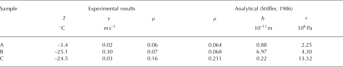
where σ is force per unit area. If it is assumed that ice asperities in contact with the steel are flattened under the load until their sum area balances the normal force and the asperities are in a state of incipient failure, then the force per unit area is equal to the penetrative hardness of ice. Reference Barnes and TaborBarnes and Tabor (1966) demonstrated that penetrative hardness of ice is dependent on temperature and the dwell period. for dwell times of the order of 10−4s, consistent with the short period that counter-facing asperities are in contact with each other, the penetrative hardness of ice at −3°C is 35 MPa and at –25°C is 63 MPa (Reference Barnes and TaborBarnes and Tabor, 1966). The fluid film thickness and µ have been calculated for the three samples examined using Equations (1) and (3) and relevant values for the penetrative hardness of ice (Table 1). The value of µ for the low-friction samples (A and B in Table 1) are in good agreement with the experimental results. However, the analytical value of µ (0.21) for sample C is larger than the experimental value (0.16) (Table 1), indicating that high friction at low temperature and low velocity cannot be described satisfactorily by lubricated friction via frictional melting alone.
Table 1. Comparison of experimental results for ice on steel with the calculations based on the analytical solution of Reference StifflerStiffler (1986) for an ice pin on a steel substrate (see Equations (1–3))
Wear morphology and the thickness of the fluid film
The morphology of wear formed during frictional sliding appears to be dependent on the thickness of the fluid film that forms at the ice–steel interface via frictional heating. The thickness of the fluid film increases non-linearly with velocity (µ∝v 3/2) and decreases linearly with temperature (see Equation (1)). At high temperature and low velocity (sample A), sufficient heat is produced to cause significant melting so that the morphology of the debris is produced by the deposition and refreezing of liquid water on the trailing edge of the wear surface. It appears that melt fluid formed at the sliding interface was swept backwards and deposited at intervals, leading to successive bands of varied morphology in the debris. This suggests that the fluid had solidified before the subsequent pulses of meltwater were deposited.
At low temperature and high velocity (sample B) the debris appears as a solid, consolidated block that lacks morphological zones. Based on the velocity and temperature of the two experiments (see Equation (1)), it is estimated that the thickness of the fluid film formed under sample B is an order of magnitude greater than under sample A (Table 1). It appears that the relatively thick fluid film was swept to the trailing edge of the wear surface of sample B where it refroze in a single event so that morphological bands are absent.
The thickness of the fluid film for the high friction at low temperature and low velocity (sample C) is calculated to be significantly less than the low-friction samples (Table 1). It appears that the film was not sufficiently thick to completely lubricate the ice–steel interface, leading to localized welding and the development of scuffing features. The shear stress at the sliding interface of sample C is an order of magnitude greater than for samples A and B (Equation (2); Table 1). The significantly higher shear stress at the sliding interface of sample C may have resulted in the brittle failure and the deposition of sheets of ice on the trailing edge of the wear surface.
Conclusion
A method for the direct observation of ice wear surfaces using LT-SEM has been successfully developed. It has been used here to identify diagnostic wear morphology that differentiates frictional processes based predominately on frictional heating and lubricated friction from those that predominately involve the brittle failure of ice. Low friction (µ < 0.1) both at high velocity–low temperature and at low velocity–high temperature is characterized by the development of a cohesive mass of debris with well-defined grain boundaries and spheroidal air bubbles indicative of the deposition and refreezing of liquid water. High friction (µ > 0.15) at low velocity–low temperature is characterized by the scuffing of the wear surface and sheets of solid debris that accumulate at the trailing edge of the wear surface, indicative of brittle failure of ice at the sliding interface. By combining LT-SEM observations of ice wear morphologies with empirical µ-v-T friction maps it will be possible to develop process-based ice wear maps for a variety of slider materials. The development of ice friction-process maps will be of great use to engineers working on structures for ice-prone environment, winter sports and traction control systems for automobiles.
Acknowledgements
This work was funded by the Engineering and Physical Sciences Research Council. The contribution of two reviewers is gratefully acknowledged.


