Introduction

The mass balance of the Antarctic ice sheet is determined by the difference between the net snow accumulation and ice discharged across the grounding line into the ocean. Most of the Antarctic ice sheet is drained by outlet glaciers and ice streams. Although only 13% of the Antarctic coastline consists of these glaciers (Reference DrewryDrewry, 1983), they discharge about 90% of the snow that falls inl!and of the coastal zone (Reference Morgan, Jacka, Akerman and ClarkeMorgan and others, 1982). The velocity field of these glaciers is a critical parameter, together with ice thickness, in determining the ice-discharge rate. The size of the glaciers and the presence of numerous crevasse fields across the ice streams make the glaciers difficult to study by traditional terrestrial field survey. Moreover, because of logistical problems and difficult environmental conditions, field research in Antarctica has focused on only a lew ice streams and outlet glaciers close to scientific stations or summer camps. Several authors have shown that ice-flow velocities can be determined through measuring the displacement of features observed in pairs of visible or synthetic aperture radar ι SAR ι images (e.g. Reference MorganMorgan, 1973; Reference Lucchitta and FergusonLucchitta and Ferguson, 1986; Bind-schadler and Scambos, 1991; Reference Lucchitta, Mullins, Allison and FerrignoLucchitta and others, 1993, Reference Lucchitta, Rosanova and Mullins1995; Reference Bindschadler, Vornberger, Blankenship, Scambos and JacobelBindschadler and others, 1996). in situ measurement of velocities has been performed using both Transit and global positioning system (GPS) techniques (e.g. Reference Thomas, MacAyeal, Eilers, Gaylord, Hayes and BentleyThomas and others, 1984; Reference Stephenson and BindschadlerStephenson and Bindschadler, 1988; Reference Jenkins and DoakeJenkins and Doake, 1991; Reference Hulbe and WhillansHulbe and Whillans, 1994), where velocity was measured by determining the position of markers at two or more times. There have been very few comparisons made between glacier ice velocities inferred from analysis of sequential satellite images and direct measurements from field surveys (Bindschadler and others, 1994, 1996).

The major outlet glaciers of Victoria Land flow into Terra Nova Bay: Reeves and Priestley Glaciers which flow together and form the Nansen Ice Sheet (the name given by the first explorers, although it is really an ice shelf), and David Glacier whose seaward extension is the Drygalski Ice Tongue (Fig. 1). These outlet glaciers drain an area of approximately 250-000 km² which includes part of Dome C and Talos Dome (Drewry, 1983). Lucchitta and others (1993) measured the velocity at 73 points on Drygalski Ice Tingue using Landsat I multispectral scanner (MSS) (1973) and Landsat thematic mapper (TM) (1988) images. The average velocity for the entire ice tongue was 700 ma⁻¹. Frezzotti (1993) measured the velocity of Drygalski Ice'longue at 75 points using Landsat 1 MSS (1973) and LandsatTM (1990) images, and found velocities ranging from 626 ± 5 to 719 ± 5 ma⁻¹. He also obtained measurements at 137 additional points using Landsat TM from 1988 and 1990, with results ranging between 136 ± 30 and 912±30 m a⁻¹. Frezzotti (1993) calculated the average velocities of Nansen Ice Sheet at 40 points, with values ranging between 120±5 and 360±5 m a⁻¹ using Landsat MSS (1972) and SPOT XS (1988) with an averaging interval of 16 years.

Recent results from remote-sensing research and field surveys have provided new ice-velocity data for David Glacier Drygalski Ice Tongue and Priestley and Reeves Glaciers. The different sets of velocity measurements inferred from satellite images are verified by comparison wit h results from repeated GPS surveys.The flow rates from GPS measurements are in good agreement with those obtained from analysis of the satellite images. Only in the outer part of Drygalski Ice Tongue do the satellite-image and GPS derived measurements show significantly different flow rates.

Fig. 1. Landsat TM image mosaic of léna Nova Bay area collected on 17 January 1990 and used as the reference image. Solid circles and cross indicate positions of GPS-surveyed markers andfeature-tracking velocity data points.

Methods and Instruments

Satellite images were acquired by Landsat 1 MSS (1973) and Landsat TM 4 and 5 (1990-92) for David Glacier-Drygalski Ice Tongue and Reeves and Priestley Glaciers, and by SPOT 1 XS (1988) for Reeves and Priestley Glaciers. AH images were provided in digital format on computer tape and were processed to eliminate scan-lines in each spectral band. To enhance the surface features of glaciers in the images and reduce noise, we generated a first-principal-component image. We measured displacements in time by comparing our reference image, the 1990 Landsat TM image, with the 1973 Landsat MSS and 1988 SPOT XS images and the 1992 Landsat TM image. We co-registered the images using 19 tic-points for the pair of Landsat TM images of 1990 and 1992 for David-Drygalski and Priestley, 18 points for Landsat TM of 1990 and Landsat MSS of 1973 for David and Drygalski, and 20 points for Landsat TM of 1992 and SPOT XS of 1988 for Reeves. We chose as image tie-points small rock outcrops a few pixels in size, close to the glaciers, at low elevation and widely scattered across the velocity-measurement area. The co-registration of images was performed using a first-order polynomial, and the data were resampled using a cubic convolution algorithm to a common pixel size of 28.5 m, the same as our reference image. The residual errors from the co-registration process range from two pixels to sub-pixel level. Since the front of Drygalski Ice Tongue extends some 90 km out to sea from the coast, fixed features are not available as tie-points in this area, hence co-registration errors can increase to the east along Drygalski IceTongue.

The displacement of surface features (crevasses, ice fronts, snowdrifts, drift plumes, etc.) in sequential images was determined using a semi-automatic procedure. Distinct features that occur in both images were first identified, then a 16 pixel by 16 pixel image chip containing a feature was extracted from each image. A comparator then determined the relative location of the feature in the two chips to quarter-pixel accuracy. From this measurement of the displacement of the feature, the average velocity for each feature point was calculated in image coordinates, knowing the time interval between the images and the pixel size (28.5 m). Time intervals for different image pairs varied from 2 to 17 years. The numbers of measured points are 750 for David Glacier-Drygalski Ice Tmgue using Landsat TM of 1990 and 1992, and 53 using Landsat MSS of 1973 and Landsat TM of 1990; 650 for Reeves Glacier-Nansen let-Sheet using SPOT XS of 1988 and Landsat TM of 1992; and 430 for Priestley Glacier using Landsat TM of 1990 and 1992 (Fig. 1).

Satellite image maps were created, with 30 m pixel spatial resolution, using the Landsat TM reference image. A geo-referenced image was generated by identifying in the image 15 ground-control points established by the Italian Antarctic Research Programme with GPS surveys. The image was rectified to a Lambert Conformai Conic cartographic projection, using a linear conversion matrix with an rms error of about two pixels. Using the same conversion matrix, the satellite-image velocity points were transformed to the same projection.

GPS surveys have proven to be very useful for measurement of glacier movement (Hulbe and Whillans, 1994; Frezzotti and others, 1997). GPS antennas and receivers may be located at station points and left there for pre-established periods of observation. GPS surveys may be carried out in static or kinematic modes. in static mode, point positions are determined by processing entire measurement sessions ranging from a few tens of minutes (fast-static mode) to many hours or days, depending on the survey's purpose, to produce a single set of coordinates corresponding to an average position for that time interval. in kinematic mode, positions are determined for each individual observation (every 1 -15 seconds depending on sampling rate). The kinematic mode allows the determination of the path followed by objects even when moving rapidly; but in order to obtain accurate positions, at least two geodetic receivers must be used, simultaneously tracking the GPS carrier phase from more than four satellites (Capra and others, 1996). One receiver remains on a fixed location (reference station), while the other (rover station) moves along the required path within a range of some tens of km from the reference station. Data processing allows computation of the rover's antenna trajectory with respect to the reference-station position (Reference Qin, Gourcvitch and KuhlQin and others, 1992). in this way the coordinates of points on the glacier are determined with respect to fixed points located on rock outcrops. The rover station is kept at a survey marker on the moving glacier for some period, and the glacier velocity and its variation with time are then determined from the time scries of coordinates.

GPS techniques, both in static and in kinematic mode, have been used to monitor David Glacier-Drygalski Ice Tongue and Reeves and Priestley Glaciers. The static mode guarantees the best possible precision, but monitored points could experience consistent horizontal movement (up to 2 ma⁻¹) and undergo considerable vertical motion on floating parts of the glacier, with oscillations related to tidal motion. in order to investigate the effect of the movement, kinematic processing was performed on the data from the same points as for the static survey. The change in the coordinates with time showed that the motion was slow and consistent, as expected with in the associated precision.

Complex logistics due to the area's morphology (long distances, long ice tongues without rocks outcropping on the sides) prevented us from using a network with more fixed points. Hughes Bluff (HB), the only reference point in the area, was used for David Glacier Drygalski Ice longue, and the reference point at Terra Nova station was used for Reeves and Priestley Glaciers (Fig. 1). Unfortunately, in such conditions the distance between the reference station and the rover antenna often exceeds the normal limit of a few tens of km range of the kinematic method. The reference stations are located 30-100 km from the glacier survey points. With these longer baselines the achievable accuracy is lower, particularly in an environment strongly affected by ionospheric disturbances and multi-path effects due to the various reflecting surfaces. Nevertheless, the GPS technique has to be considered currently a very powerful positioning tool for surveys in Antarctica (Vittuari, 1994).

Limitations are imposed on the measurement programme by the restricted range of the helicopters used for deployment of receivers, the frequency with which they can be relocated, bad weather and other logistical difficulties. An increased number of connections to reference stations would augment the number of observation days, enabling a compromise to be made between scientific goals and the constraints of time and cost. The deployment of a number of mobile receivers at any230. one time permits an examination of the value of multiple baselines between the different occupied points. The survey instrumentation consisted of four geodetic GPS receivers (Trimble 1000 SSE) with antennas positioned on 13 cm diameter, 3 m long, aluminium poles driven into the snow or ice to about 1.5 m. Data processing was performed with Geotracer GPS v.2.25 software, which is able to process both static and kinematic observations.

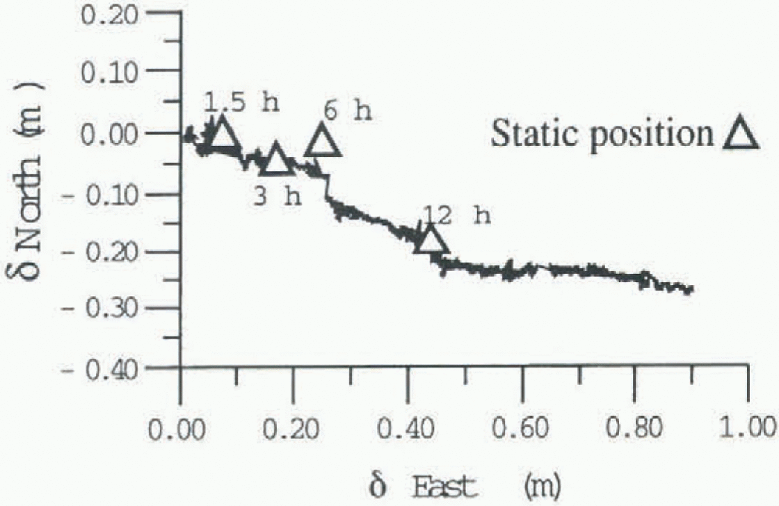
Fig. 2. Comparison between the continuous kinematic profile and the static (single baseline) positions during 12 hours of GPS acquisition.

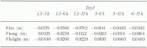
GPS observations were made at the different points over periods of 21-18 hours. To investigate the effect of movement of the antenna during the measurement session, a 12 hour interval of observations for point Dryl in November 1993 was processed in kinematic mode and the same data processed in static mode for the baseline HB-Dryl with sessions lasting 1.5, 3, 6 and 12 hours with a common start time. Results presented in Figure 2 show that planimetrie coordinates from the static solutions have values around the average position for the overall processed period, even though motion occurred during the measurement periods. When comparing the static planimetrìe positions with the continuous kinematic profile, we found that the static positions correspond to the position at the middle of the processed period to within an error which is comparable with the method's precision (5-10cm) for those baseline distances. Verification of this result was obtained using static mode for the HB-Dryl baseline for the same set of session durations (1.5, 3, 6, 12 hours), but with each session centred on the same instant. The aim of this test was to verify that the position obtained with observation periods of increasing duration would remain centred on the planimetrie position determined at the time corresponding to the middle of the overall period. The values differ from the average by amounts with in the method's precision (Table 1).

Figure 3 shows the variation ofelevation with time from the kinematic solution for point Dry 1. We note that the GPS results have detected the tidal response of the glacier. The results given in Figure 2 and Table 1 clearly show that the vertical oscillation and horizontal movement do not significantly Influence the result of Static processing of the baseline and its associated precision. The precision achieved may-appear to be inconsistent with the magnitude of the vertical and horizontal motions which occurred during the measurement period. However, the measurements acquired during the 12 hours correspond to very many single-epoch observations (2880), which stabilise the rms error even with significant point position variations.

Table 1. Difference between the coordinates obtained through single-baseline solutions at time interrali cent

Another test was performed by processing in static mode the triangle made by the independent baselines HB-Dryl— Dry8, which allows redundant observation schemes through successive sessions. But a static network cannot be determined since both points Dryl and Dry8 are moving. The processing scheme was applied to the triangle observation periods of 1.5, 3, 6 and 12 hours for two different measurement sets collected in November 1993 and November 1994. Table 2 presents the results as differences between the single-baseline static and network solutions obtained for the same acquisition intervals. Differences in the coordinate values are small and comparable to the method's precision. The precision appears to be of the same order. Since any baseline is subject to movement, and we may be unable to obtain redundant observations in these dynamic conditions, we have chosen to use only the single-baseline solutions in our discussion. The tests showed that sufficiently reliable coordinate values may be obtained from the static solution of the baseline, while ignoring the effect of movement during the observation period, making observations for a period appropriate to the baseline length and noting that the resultant position corresponds to the middle of the observation period. Considering the average error of GPS position, we can assume an error in our average velocity determination of 0.06-0.16 m a⁻¹.

Satellite-image velocity measurements are more abundant and precise in areas exhibiting extensive crevassing, but GPS measurement stations have been located, for safety, in areas where crevasses are scarce. Therefore direct comparison of velocities at identical geographic locations is noi possible. in the following discussion the closest measurements acquired by the two methods have been used.

Discussion

David Glacier is formed by the convergence of several streams below an iccfall, the David Cauldron. At this location it is possible to infer a change in the trend of the subglaciol stratum (Mclntyre, 1985), with the stream entering a deep fjord-like valley. Frezzotti (1993) pointed out that in the satellite images the grounding line was in the Mount Priestley section and that the Drygalski lec'longue was fed by two streams from David Cauldron, a northern stream and a faster southern one. The GPS stations on David Glacier (Fig. 1; Table 3) are upstream of David Cauldron (Da3 and Da5 and close to the grounding line (Da4 and Da6). Da3 and Da4 were located on the faster, southern stream while Da5 and Da6 were located on the slower, northern one. Da2, Dryl, Dry8 and Dry7 are on the floating part of David Glacier Drygalski Ice longue. We measured the behaviour of floating ice in response to the ocean tide, in order to confirm the grounding-line position, using continuous kinematic measurements performed for 24 hours at five points on Drygalski Ice Tongue-David Glacier. Points Dryl, Dry8 and Dry7 on Drygalski IceTongue exhibit on 23 October 1993 (day 296) a tidal cycle of about 50-60 cm, with two synchronous peaks that demonstrated complete hydrostatic equilibrium of the ice tongue at these points. The Da2 curve mimics the Dryl curve, but with lower amplitude (30cm) of the vertical movement that could relate to the effect of stress along the wall of a fjord-like valley or to a lower-amplitude tidal cycle inside the fjord-like valley. Point Da4 on David Glacier shows on 29 October 1993 (day 302) a tidal cycle of about 10 cm, with a peak that is synchronous only with maximum tide observed in Dryl and which therefore should be located in the tidal flexure area upstream of the grounding line. New satellite-image and GPS measurements confirm the slower ice velocity of the northern stream, with a velocity at the grounding line for the southern stream of 510-560 m a⁻¹ , and for the northern stream of 70-150 m a⁻¹. Figure 4 shows the ice velocity increases significantly from the icefall to about halfway along the ice tongue, from which location, based on GPS data (Dry8 and Dry7), it remains constant to the terminus.

figures 4 and 5 show a very good agreement between values determined by feature-tracking (LandsatTM 1990-92) and GPS survey (1991-94) along David Glacier and the first part of Drygalski Ice Tongue. The difference between velocities obtained through feature-tracking almost coincides with GPS measurements, in both azimuth and velocity, for Da4, Da3, Da5 and Dryl, with differences in azimuth of 8-10° and < 15 m ⁻¹ difference in velocity.

Table 2. Comparison between the coordinates obtained through network and single-baseline solutions computed for Dryl and Dry8 points at different time intervals. Data are referred to 1994 measurements

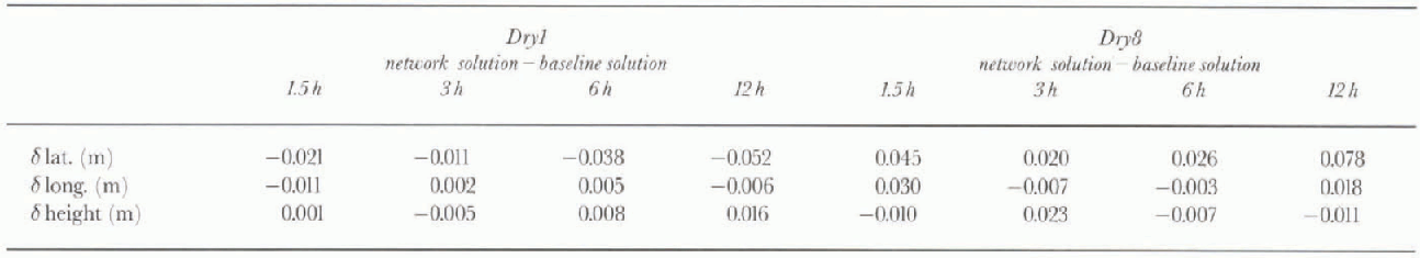
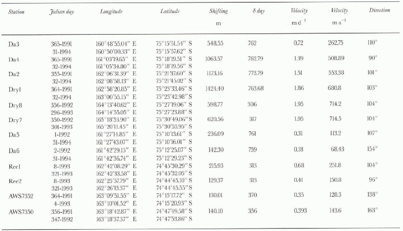
Table 3. GPS station, coordinate, time interval and velocity used in this paper

For Da2 and Da6, GPS velocities agree fairly well with the pattern of velocity variations detectable by feature-tracking, even though there are no measurements from the two methods in close proximity. For Dry8 and especially Dry7, we note differences of 30-70 m a⁻¹ between the two measurement methods. This substantial difference must be connected with a lack of sharply defined features in the outer part of the Drygalski IceTongue and with error propagation from the co-registration of the satellite images.

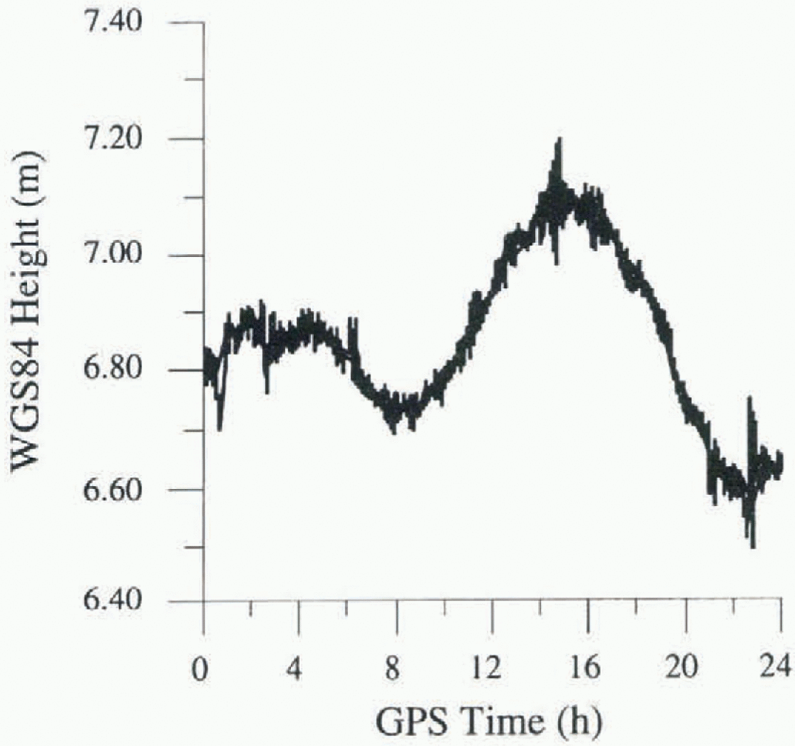
Fig. 3. Vertical displacement of a GPS station located on the Drygalski Ice Tongue due to the ocean tidal motion. The first 12 hours refer to the same period as shown in Figure 2.

Comparison between velocity measurements by GPS and feature-tracking between Landsat MSS (1973) and Landsat TM (1990) shows a good accordance in the outer part of the ice tongue, with velocity differences of the order of tens of ma⁻¹.

Where Reeves Glacier flows into Nansen Ice Sheet it divides into three streams because of the interaction with Teall Nunatak and with buried topography, which creates the divergence (Reference Baroni, Frezzotti, Giraudi and OrombelliBaroni and others, 1991). Frezzotti and others (1996) located the grounding line downstream of this topography. GPS stations (Reel and Ree2) were occupied in January and November 1993 (Table 3), and were located in the northern stream, Reel upstream and Ree2 downstream of the grounding line (Fig. 1). Comparison between velocities measured by feature-tracking (SPOT XS 1988 and Landsat TM 1992) and GPS survey shows (figs 5 and 6) a fairly good agreement, within 5-20° in azimuth and about 30 m ain velocity. The considerable difference in azimuth for point Reel and neighbouring feature-tracking results (fig. 5b) is related to the high variability of the flow in the area, due to direction and slope variations.

Priestley Glacier flows into Nansen Ice Sheet from the north. Frezzotti and others (1996) placed the grounding line close to Black Ridge where the glacier curves towards the south. GPS stations (AWS 7350 and AWS 7352) were established in conjunction with the Italian automatic weather stations 7350 and 7352. The first station was located on Nansen Ice Sheet on the stream emanating from Priestley Glacier (AWS 7350), and the second on Priestley Glacier within its valley. Comparison between velocities measured with Landsat TM (1990-92) and data acquired by GPS survey AWS 7352 (1990 91) shows a good match, with dilfer-ences of less than 10 m a⁻¹ and 10° in azimuth (figs 5 and 7). The area immediately surrounding AWS 7350 on Nansen Ice Sheet docs not exhibit features that can be tracked in satellite images, but the GPS velocity is in good agreement with velocities derived by feature-tracking in neighbouring areas.

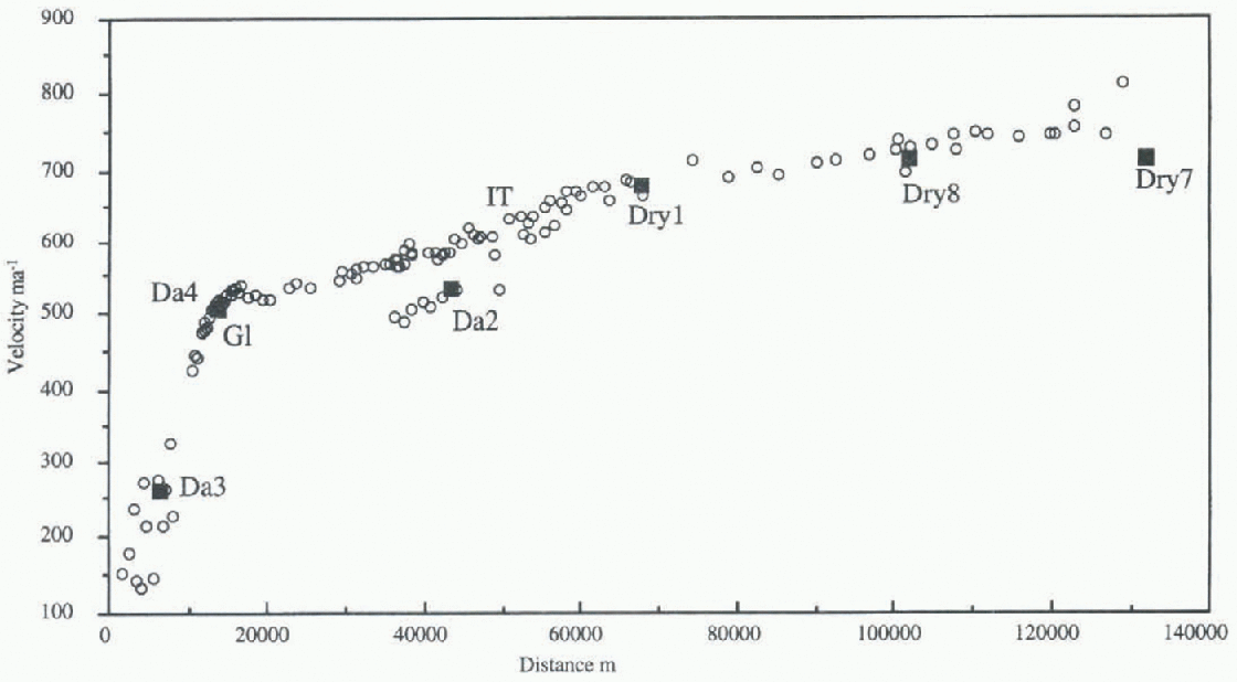
Fig. 4. Ice velocity along a corridor (1.5-12 km wide) on David Glacier Drygalski Ice Tongue following the southern stream. Solid squares are surface GPS survey velocity, and open circles are image-derived velocity from TS 11990 and 1992 (Gl. grounding line; IT, ice tongue).

Comparison of velocities measured by GPS survey and feature-tracking techniques shows good agreement in areas near image tic-points, with differences generali) much lower than the pixel size of 28.5 m. Comparison between velocities l'rom GPS survey and feature-tracking acquired at almost coincident points Da3, Da4, Da5, Dryl, Dry 8, Reel, Ree2 and AWS 7352 shows a maximum difference of about 15 20 m a⁻¹. Many authors (e.g. Bindschadler and Scambos, 1991; Frezzotti, 1993; Lucchitta and others, 1993, 1995) have suggested that the error determination in measurements is close to satellite pixel resolution, i.e. about 30 m for Landsat TM. This analysis appears to confirm and even improve on this hypothesis. Bindschadler and Scambos (1991) used for the co-registration of images the topographic-undulations of the ice stream, thus allowing co-registration even in areas lacking discrete or sharply defined lie-points.

Comparison between velocities from GPS survey and feature-tracking in images acquired by Landsat MSS and Landsat TM 17 years apart shows good agreement (Fig. 5). The limiting factor in the use of images acquired over such long time intervals is that trackable morphological features are present and reta in their identity only on some glaciers or glacier tongues and normally at a considerable distance from the grounding line (Lucchitta and others, 1995). Lucchitta and others (1995) showed flow new-generation ERS-1/2 satellites with high-resolution satellite-borne imaging SAR may allow identification of small crevasses and other patterns on ice streams or ice sheets above or at the grounding line. Ice velocity can be determined also with satellite-borne imaging SAR interferometry even in featureless areas (Reference Goldstein, Engelhardt, Kamb and FrolichGoldstein and others, 1993). Estimated errors of ± 15 20 m a⁻¹ in determination of velocity could be significantly high for small outlet glaciers with velocities of about 100-200 ma⁻¹ (10 15%) but are certainly oflittlc significance for most of the major outlet glaciers with velocities of 400-1000 m a⁻¹. Bindschadler and others (1996; evaluated the ice thickness of Ice Streams D and E through airborne ice-penetrating radar and GPS, and assumed a systematic error in ice-thickness measurement of ± 10 m. Drewry (1983) determined that ice-stream and outlet glaciers represent about 3954 km of the Antarctic coastline. Using a systematic error of ± 20 m a⁻¹ for determ i-nation of ice velocity through feature-tracking and ±10 m for ice thickness with ice density of 917 kg m ³, we can estimate a measurement error of ice discharge at the grounding line of about ±100Gta , representing about 5% of snow accumulation (1660 Gt a⁻¹) in the grounded area (Reference Bentley, Giovinetto, Weiler, Wilson and SeverinBentley and Giovinetto, 1991).

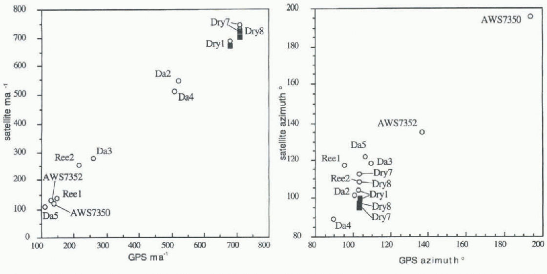
Fig. 5. Comparison of velocity and azimuth derived from feature-tracking and GPS in situ measurements. Solid circles arefrom TAI and TM-SPOT image-derived velocities, and solid squares are from MSS-TM image-derived velocities.

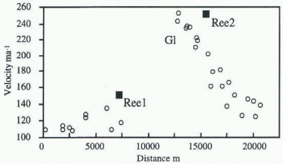
Fig. 6. Ice velocity along a corridor (0.5-2 km wide) on Reeves Glacier following the northern stream. Solid squares are surface GPS survey velocity, and open circles are image-derived velocity from the. SPOT XS 1988 and Landsat TM 1992.

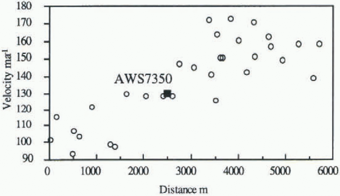
Fig. 7. Ice velocity along a corridor (2 km wide) on Priestley Glacier following the ßow. Solid squares are surface GPS survey velocity, and open circles are image-derived velocity fromTM 1990 and 1992.