


1. Introduction
The Greenland ice sheet has been losing mass at an accelerating pace over the past two decades (Reference Rignot, Velicogna, Van den Broeke, Monaghan and LenaertsRignot and others, 2011). A mass balance of –234 ± 20 Gt a–1 (April 2002 to February 2012) was derived from Gravity Recovery and Climate Experiment (GRACE) data (Reference Barletta, Sørensen and ForsbergBarletta and others, 2013). At least half of this mass loss is attributed to a reduction in the surface mass balance (SMB) (Van den Broeke and others, 2009). This is in part due to an increase in melt area (Reference Fettweis, Tedesco, Van den Broeke and EttemaFettweis and others, 2011). During warm summer periods, such as July 2012, surface melt can occur across almost the entire ice sheet (Reference NghiemNghiem and others, 2012). Melt has increased due to the long-known atmospheric warming in Greenland (Reference BoxBox, 2002) and in recent years has been amplified by atmospheric and oceanic conditions favouring high pressure over Greenland, such as a negative North Atlantic Oscillation (NAO) index (Reference Fettweis, Hanna, Lang, Belleflamme, Erpicum and GalléeFettweis and others, 2013; Reference HannaHanna and others, 2013). Owing to the increased melt, the ice sheet’s surface albedo is declining (Reference Box, Fettweis, Stroeve, Tedesco, Hall and SteffenBox and others, 2012), resulting in larger solar radiation absorption and thus stronger melt (melt–albedo feedback).
When investigating the causes of mass loss from the Greenland ice sheet, it is important to distinguish between regions, as atmospheric and oceanic impacts on ice dynamics and SMB are spatially highly variable. For instance, compared with the east coast, the west of the ice sheet has exhibited strong warming associated with changes in the summer general circulation (Reference Fettweis, Hanna, Lang, Belleflamme, Erpicum and GalléeFettweis and others, 2013) and causing mass loss in recent years (Reference SasgenSasgen and others, 2012). In this study we focus on the Godthåbsfjord/Nuuk region in southwest Greenland (Fig. 1). This area has undergone intermittent but substantial glacier shrinkage since the 18th century; Kangiata Nunaata Sermia (KNS) has retreated >20 km since the Little Ice Age (Reference Weidick, Bennike, Citterio and Nørgaard-PedersenWeidick and others, 2012). Glacier mass loss yields increased freshwater inflow into the fjord by enhanced runoff and/or calving. Reference MortensenMortensen and others, (2013) showed that the glacial meltwater greatly impacts the fjord’s salinity and circulation, which in turn controls frontal ablation of marine-terminating glaciers.
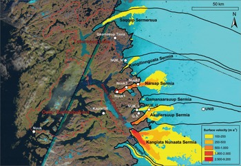
Fig. 1. Drainage basins and surface velocities in the Nuuk region of Greenland overlain on Landsat imagery from 1999–2002 and RADARSAT-derived surface velocities for winter 2005/06. Dots indicate weather station locations.
Our aim is to assess and explain the changes in SMB of the glacial catchments in the Nuuk region over recent decades. This provides us with freshwater runoff estimates, which are vital to studies of fjord circulation, given that annual glacier runoff equals roughly one-tenth of the water in the entire inner fjord. Automatic weather station (AWS) data can be used to explicitly resolve the surface energy and mass balance of ice sheets (Reference AndersenAndersen and others, 2010; Reference Van den Broeke, Smeets and Van de WalVan den Broeke and others, 2011; Reference Van AngelenVan As and others, 2012). However, there is a limit to spatial extrapolation of meteorological observations, as correlation is lost with increasing distance (Reference BoxBox, 2002). In this study we therefore rely on two regional climate models (RCMs): the Modèle Atmosphérique Régional (MAR, version 3.2) and the Regional Atmospheric Climate Model (RACMO2). These RCMs have proven to be valuable tools for estimating Greenland ice sheet SMB (Reference EttemaEttema and others, 2009; Reference Fettweis, Tedesco, Van den Broeke and EttemaFettweis and others, 2011).
To be able to obtain meltwater runoff and SMB estimates for the Nuuk region, we first delineate catchments. RCM output is resampled to a fine grid spacing so that the modelled ice masks closely match the actual ice-covered area in this region, with outlet glaciers that are narrow compared with the native grid spacings of the RCMs. We evaluate model performance with AWS observations and discharge measurements from a proglacial lake that collects meltwater from the ice sheet.
2. Methods
2.1. Area of interest and catchment delineation
The Godthåbsfjord/Nuuk region of Greenland (63–66° N, 44–53° W) (Fig. 1) is a mountainous fjord system that borders a section of the ice sheet spanning ~46 200 km2, 2.6% of the Greenland ice sheet area. The marginal region of the ice sheet consists of six outlet glaciers named:
-
Saqqap Sermersua (SS), land-terminating
-
Kangilinnguata Sermia (KS), land-terminating
-
Narsap Sermia (NS), marine-terminating
-
Qamanaarsuup Sermia (QS), land-terminating
-
Akullersuup Sermia (AS), marine-terminating
-
Kangiata Nunaata Sermia (KNS), marine-terminating
The meltwater from SS first collects in Tasersuaq Lake (TL; Fig. 1). The ice-dammed Isvand Lake (IL) currently drains underneath KNS into Godthåbsfjord. Until 2004 its water level was high enough to overspill into Austmannadalen, a valley that has no direct hydrological connection to Godthåbsfjord (Reference Weidick and CitterioWeidick and Citterio, 2011).
By delineating the hydrological drainage basins we can determine the freshwater fluxes at the multiple entry points to the inner Godthåbsfjord (GFI), and thus the total flux into the outer fjord (GFO). This is done using the Advanced Space-borne Thermal Emission and Reflection Radiometer (ASTER) digital elevation model (DEM) (Reference Hvidegaard, Sørensen and ForsbergHvidegaard and others, 2012) and aerial photography. Over the ice sheet, a topographical delineation may lead to large errors in the catchment delineation at high elevation, partly because standard hydrological tools in software packages such as ArcGIS are inaccurate over large smooth surfaces (Reference Van AngelenVan As and others, 2012). Furthermore, in southwest Greenland, surface melt-water does not run off along the ice-sheet surface. Before reaching the margin, the meltwater flows into moulins and crevasses that conduct it to the glacier bed. This implies an influence of subglacial topography. Since a sufficiently accurate bedrock map does not exist, we delineate the glacier catchment from the 2005/06 RADARSAT surface velocity map (Reference Joughin, Smith, Howat, Scambos and MoonJoughin and others, 2010) using the ArcGIS particle track function. We implicitly assume that the direction of ice flow is a function of both surface and bottom topography. With this method the glaciers are delineated dynamically as well as hydrologically, allowing us to study their mass budgets and freshwater contributions to the fjord.
2.2. RCMs and resampling
To determine the SMB components for the study region we use output of the two meteorological models MARv3.2 and RACMO2. Both RCMs include a surface layer of snow and ice two-way coupled to the atmosphere to allow for realistic calculation of the surface energy and mass fluxes at the ice– atmosphere interface. This makes it possible to estimate meltwater refreezing in the snowpack (Reference Reijmer, Van den Broeke, Fettweis, Ettema and StapReijmer and others, 2012) and subsurface heat and mass fluxes on a multilevel grid. Also, the models calculate albedo change due to snow metamorphosis and bare-ice appearance (Reference RaeRae and others, 2012), a first-order feedback on surface melt (Box and others, (2012). Minimum values are set to 0.4 for MARv3.2 and to a remotely sensed minimum albedo field for RACMO2 (Reference Van AngelenVan Angelen and others, 2012). Both RCMs are forced at the boundaries by European Centre for Medium-Range Weather Forecasts (ECMWF) reanalysis data (Reference DeeDee and others, 2011). The longest period for which both models have results is 1960–2012, defining our study period. For details on MARv2 and RACMO2 physics we refer to Reference Fettweis, Tedesco, Van den Broeke and EttemaFettweis and others, (2011) and Reference Van AngelenVan Angelen and others, (2012), respectively. The former is upgraded to MARv3.2 with a new ice-sheet topography and mask, in addition to improvements in cloud micro-physics reducing precipitation. MARv3.2 is run at 25 km and RACMO2 at 11 km horizontal grid resolution.
We do not make use of the models’ ice mask fractional cover along the ice-sheet margin in order to eliminate this potential cause of model disagreement, but use the outlines as determined from recent Landsat imagery. However, the RCM grids do not resolve the 1.5–5.0 km wide outlet glaciers in the Nuuk sector of the Greenland ice sheet (Fig. 2), while the SMB components such as melt on the unresolved glacier areas likely are substantial. We address this by means of bilinear interpolation to a finer grid, chosen to have a 250 m resolution that fully resolves the narrowest glacier in the region. For this resampling, only same-surface-type gridpoints were used, i.e. the values at resampled ice surface points are determined using on-ice values only and not tundra values.
Fig. 2. Catchments from Figure 1 (black lines) overlain by RCM grids. MARv3.2 (blue) grid spacing is 25 km, and RACMO2 (red) grid spacing is 11 km. Dots represent partial or full ice cover in the model masks; crosses (+) represent tundra and fjord.
2.3. Model evaluation by observations
Meteorological measurements in Nuuk date back to the 18th century (Reference Vinther, Andersen, Jones, Briffa and CappelenVinther and others, 2006). In recent decades more weather records on land have been obtained by the Danish Meteorological Institute (DMI), Asiaq (Greenland Survey) and the Greenland Airports (GL). The 13 weather stations selected for this study are positioned within the catchments mentioned above (Table 1). On the ice sheet, the first continuous and still ongoing measurements within the hydrological catchment of Godthåbsfjord were performed as part of the Greenland Climate Network (GC-Net) (Reference Steffen, Box and AbdalatiSteffen and others, 1996) in 1997. Several more stations have been erected since, among which three are in the ablation zone for the Programme for Monitoring the Greenland Ice Sheet (PROMICE) (Reference Van AsVan As and others, 2013). Here we summarize a detailed RCM evaluation using AWS observations. Modelled SMB is evaluated in Section 3.
Table 1. Metadata for selected automated weather observations within the study region and period. Weather stations below the dividing line were/are positioned on the ice sheet
Variability of daily mean near-surface air temperature is captured well by the models, with correlation coefficients (r) exceeding 0.95 at all stations except one. Root-mean-square errors (RMSEs) range from 2°C to 8°C, partly explicable by differences in actual and model site elevations. Correlation coefficients for air pressure are high (0.97–0.99). For wind speed, correlation coefficients are lower, down to 0.6, with mean errors in the order of 1 m s–1. Downward shortwave radiation is relatively accurate, with no clear offset and RMSE values close to the measurement uncertainties of the radiometers. Summer ice-sheet albedo is overestimated by the RCMs at nearly all sites, which will directly influence melt calculations due to reduced absorption of shortwave radiation. Downward longwave radiation is underestimated by the RCMs by ~10–30 W m–2 at all sites, also causing calculated melt to be underestimated.
The selected AWSs on land are equipped with precipitation gauges, allowing for an evaluation of modelled precipitation. The uncertainties in (especially solid) precipitation measurements are large, with known examples of measurement errors of up to 100% (Reference Allerup, Madsen and VejenAllerup and others, 1997). For Greenland, wind-induced undercatch is evaluated to be the greatest error source (Reference Yang, Ishia, Goodison and GuntherYang and others, 1999). In spite of this, both models calculate (up to a factor of four) lower precipitation values than observed at most sites, though not for the orographically sheltered Kapisillit site, where the models overestimate precipitation. This is illustrative of difficulties in calculating and measuring precipitation, especially in a mountainous region. Comparison with AWS measurements on the ice sheet is provided in Section 3.1. Over the flat accumulation zone of the ice sheet, a detailed comparison between observed and modelled snow accumulation showed good agreement (Reference EttemaEttema and others, 2009).
Finally, RCM runoff from the SS catchment is evaluated using measured discharge at Tasersuaq Lake in Section 3.1, thus comparing area totals rather than local values. The water level in the lake was monitored from 1974 to 1983 and again from 2008 to 2012. Water level is converted into discharge values by a stage–discharge relation, based on manual measurements of discharge over a range of water levels. The scatter in the single stage–discharge measurements yields an uncertainty of 6% for single values.
3. Results
3.1. Observed versus modelled SMB and runoff
Most on-ice stations are equipped with sonic height rangers, which record surface height change resulting from accumulation and ablation. The Geological Survey of Denmark and Greenland (GEUS) stations additionally make use of a pressure transducer assembly (Reference Fausto, Van As, Ahlstrøm and CitterioFausto and others, 2012). Figure 3 shows a comparison of measured and modelled surface height change in the lower ablation area (NUK_L) and in the upper accumulation area (South Dome). Modelled surface height change is calculated as snowfall reduced by sublimation, evaporation and melt, bilinearly interpolated to the AWS location. It does not include refreezing, which occurs below the surface. Differences between models and observations are significant. At NUK_L, where 5–7 m of ice ablates per year, the models underestimate net ablation by ~30–50%, which cannot be explained fully by small-scale variability in ablation as seen from local stake measurements (Reference BraithwaiteBraithwaite, 1986). The difference is mainly due to overestimated accumulation and bare-ice albedo. The lack of winter accumulation on the QS outlet below ~900 m elevation was reported by Reference BraithwaiteBraithwaite, (1986) and is likely due to orographic sheltering and snow being blown into surface depressions and crevasses, thus not accumulating underneath the instruments. A similar lack of accumulation was reported for the marginal ice sheet near Kangerlussuaq (Reference Van AngelenVan As and others, 2012). In the accumulation area (South Dome), the surface height increase is larger in MARv3.2 than in RACMO2 due to differences in snowfall. Depending on the snow density used to convert the measurement into comparable units (here 350 kg m–3; Reference BoxBox, 2001), also at this site the mass budget disagrees with measurements by up to 30%.
Fig. 3. Cumulative surface height change due to accumulation and ablation at the NUK_L and South Dome on-ice weather stations. Black lines: observations; blue lines: MARv3.2; red lines: RACMO2. For conversion of surface height change measurements into w.e. a snow/ice density of 350/900 kg m–3 is used
Model performance improves on the catchment scale; this is illustrated in Figure 4, which compares discharge measurements at the TL river outlet with daily catchment totals for modelled runoff from SS. We applied a 1 week delay and 15 day smoothing to RACMO2 runoff values to represent (in basic form and for plotting purposes only) meltwater routing delays. MARv3.2 calculates a runoff delay following Reference Zuo and OerlemansZuo and Oerlemans, (1996). Both models produce realistic runoff quantities and temporal variability therein, although there is evidence to suggest that runoff is underestimated in the high-melt years 2010–12. The agreement with discharge observations is reduced when modelled runoff from the tundra TL catchment, which peaks in spring when snow melts, is also taken into account. Many of the smaller lakes in the TL catchment may not drain into Tasersuaq Lake, their main sinks being evaporation and/or interaction with groundwater. More importantly, the TL measurements do not reveal the runoff used for the 7 m water level increase in spring. The nonzero lake discharge values in autumn and winter are similarly the result of lake volume decrease, but could also be due to englacial storage (Reference RennermalmRennermalm and others, 2013), or melt- and rainwater from the tundra reaching the lake with delay due to groundwater interaction.
Fig. 4. Observed discharge from Tasersuaq Lake (black), and runoff as calculated by MARv3.2 (blue) and RACMO2 (red) for catchment SS.
In conclusion, for single locations, errors and uncertainties in RCMs as well as observations can prevent a useful comparison, as seen at the AWS sites. However, integrating the data over the scale of a glacial catchment produces improved agreement between models and observations.
3.2. Melt, runoff and SMB in the Nuuk region of the ice sheet
The pronounced annual cycle in Figure 4 is due to melt, which is confined to the warm season. Figure 5b illustrates that ice-sheet melt in the Nuuk region occurs chiefly in May–September, peaking at >10 km3 w.e. in July (1960–2012 average). Since rainfall (Fig. 5a) has the same seasonality, though approximately a factor of ten smaller in magnitude, this is also valid for runoff (Fig. 5d). Runoff equals meltwater and rainwater combined, reduced by what is refrozen in snow and firn (Fig. 5c). According to the two models, in the period 1960–2012, almost half of all liquid water refroze.
Fig. 5. Mean annual cycles of snowfall and rainfall (a), melt (b), refreezing (c), runoff (d), evaporation and sublimation (e) and SMB (f) calculated by MARv3.2 (blue) and RACMO2 (red) for the Nuuk region of the ice sheet for 1960–2012.
The SMB for the region is calculated as snowfall – sublimation/evaporation – melt + refrozen mass (equal to precipitation – sublimation/evaporation – runoff). The average SMB is negative in June, July and August (Fig. 5f). Snow accumulates in the higher regions of the catchments throughout the year, peaking slightly in autumn, so melt mostly forces the yearly cycle in SMB. Regionally, sublimation and evaporation contribute little to the SMB (Fig. 5e).
Annual total values for 1960–2012 are illustrated in Figure 6. Surface melt increased from an average of 20–25 km3 a–1 w.e. from 1960 to the mid-1990s to values 50–150% higher in recent years (Fig. 6b). The melt increase is well documented: 2007 was the strongest melt year on record (Reference Tedesco, Serreze and FettweisTedesco and others, 2008) until 2010 (Reference TedescoTedesco and others, 2011; Reference Van AngelenVan As and others, 2012), which was surpassed by 2012 (Reference TedescoTedesco and others, 2013). In the Nuuk region, >50 km3 of meltwater was generated in 2012.
Fig. 6. Same as Figure 5, but annual totals. The solid black line illustrates the 5 year running mean for both models combined.
The amount of melt- and rainwater that was calculated to refreeze remained stable at 10–15 km3 w.e. throughout the period (with 2012 as an outlier), causing runoff to increase relatively more than melt (Fig. 6d). Although rainfall also increased during the 53 year period, it contributes <5 km3 w.e. a–1.
The SS catchment produces most runoff in the Nuuk region (Table 2), with a mean contribution of 31% or 41%, depending on the model used. Whereas the models calculate very similar SMB components in the SS catchment (e.g. average melt within 5% and runoff within 2%), in most other catchments MARv3.2 gives higher melt (12%) and less refrozen mass (16%) than RACMO2. This is on average accompanied by (and presumably also caused by) lower solid precipitation values (17%). The models calculate that there is no trend in the relative runoff contributions from the catchments, as indicated by the small standard deviations in Table 2. This suggests that runoff from the catchments reacts similarly to climate forcing, in spite of the different catchment shapes. More importantly, this means that it suffices to monitor the runoff from one catchment (as at Tasersuaq Lake) to be able to estimate the annual freshwater discharge into Godthåbsfjord from all catchments. However, the models do not agree on the relative contributions from the catchments (Table 2), and this requires further study.
Table 2. Contributions from catchments to the runoff from the Nuuk ice sheet region, including standard deviation calculated from annual totals
When calculating the hydrological contribution of KNS to Godthåbsfjord a complicating factor is that the ice-sheet region IL, which drains water into the ice-dammed Isvand Lake, is dynamically part of KNS, but hydrologically only partly so. After the formation of the lake in the 18th century, the lake water spilled over into Austmannadalen and flowed into Ameralik Fjord, which has no direct connection to Godthåbsfjord. From 2004 onwards, the lake exhibited sudden drainages through the KNS englacial conduit system, until in recent years it lost hydrological connection to Ameralik Fjord altogether. These changes in the lake’s hydrological pathways are related to thinning of KNS (Reference Weidick and CitterioWeidick and Citterio, 2011). For the hydrology of Godthåbsfjord, this implies that in recent years KNS runoff increased, receiving a larger share of IL runoff, which is a model average of 20% of the KNS value for 1960–2012. As with all ice-dammed (or supraglacial) lakes in the region, the timing of freshwater release due to episodic drainages cannot be modelled with accuracy and is therefore not discussed here.
Compared with the runoff from the ice sheet, the three mostly ice-free catchments of TL, GFI and GFO produce small but non-negligible freshwater fluxes. The catchments receive mean annual precipitation quantities of 2.2, 2.0 and 1.8 km3 for 1960–2012 according to MARv3.2, and 2.6, 3.4 and 3.3 km3 according to RACMO2. In low-melt years the modelled precipitation in the ice-free catchments exceeds the total runoff from the ice sheet. However, as discussed with Figure 4, it is not known how much of this makes it to the fjord, and when.
With snowfall on the ice sheet in the region unchanging throughout the period 1960–2012 (Fig. 6a), and mass loss/gain due to sublimation and evaporation being an order of magnitude smaller than the other SMB components, the changes in regional SMB during the study period are the result of melt. Throughout most of the period, SMB was positive and trendless at 10–15 km3 w.e. a–1 on average, with precipitation causing most of the interannual variability. The trend changed around 2000 when melt started increasing, causing SMB to decrease. This melt increase is a consequence of an increase in negative phases of the NAO, favouring warmer and drier summers over the ice sheet (Reference Fettweis, Hanna, Lang, Belleflamme, Erpicum and GalléeFettweis and others, 2013). Since the end of the 1990s, the occurrence of anticyclones centred over the ice sheet has doubled, which induces more frequent southerly warm air advection along the western Greenland coast. In recent extreme melt years this led to a negative modelled SMB. In the warm year 2010, the average SMB for the region was calculated to be –6.7 km3 w.e., with models in agreement. In 2012, for which an average SMB of –0.9 km3 w.e. is calculated, the model values differ by nearly 20 km3 w.e. due to differences in solid precipitation and refreezing. In the long-term perspective given in Figure 6c it is likely that model-average refreezing is overestimated in 2012, and that the annual SMB is more similar to that of 2010.
The three marine-terminating glaciers NS, AS and KNS contributed to additional regional mass loss due to frontal ablation (calving + melt). Accurate frontal ablation is known only for KNS, as this is the only glacier in this region for which there is some knowledge of bed topography (Reference GogineniGogineni, 2012). Five values, based on remotely sensed wintertime surface velocity maps (Reference Joughin, Smith, Howat, Scambos and MoonJoughin and others, 2010), increased by 10% to account for spring/summer speed-up (Reference AhlstrømAhlstrøm and others, 2013) are plotted with the SMB values for KNS in Figure 7. The SMB trend is similar to that for the entire ice-sheet region (Fig. 6f), since KNS makes up 42% of the ice-covered region, but annual values are positive throughout. Taking into account the frontal ablation of KNS, the data imply that KNS was gaining mass until about 2007. Reference Rignot and KanagaratnamRignot and Kanagaratnam, (2006) reported that KNS accelerated by 6% from 1996 to 2000 and by another 27% by 2005. This makes it unlikely that frontal ablation could have balanced the positive SMB before 1996 (Fig. 7), also implying a mass gain. Since the outlet glaciers in the region are unlikely to have thickened or lengthened during this period (Reference Weidick, Bennike, Citterio and Nørgaard-PedersenWeidick and others, 2012), this means that either the ice sheet was gaining mass in the accumulation area, or that the SMB is overestimated by the RCMs. If the former is true, the model average mass balance for KNS was ~-2 to –4 km3 w.e. a–1 for 2010–12. However, the model evaluation in this study shows that melt is underestimated, and that precipitation/accumulation may be overestimated, which would justify a downward adjustment of the SMB values. If we assume more realistically that KNS was at balance during 1961–90, a commonly used climatic reference period (dotted line denoting the SMB equilibrium level in Fig. 7), the glacier lost 5–6 km3 w.e. in 2010, the equivalent of a mean surface lowering of ~0.3 m w.e.
Fig. 7. SMB for the KNS + IL catchment as calculated by MARv3.2 (blue) and RACMO2 (red). Frontal ablation (calving + melt) estimates for KNS are indicated by crosses (+), with their vertical extent indicating the uncertainty. These wintertime RADARSAT-derived dynamic fluxes were increased by 10% to better represent the annual mean flux (Reference AhlstrømAhlstrøm and others, 2013). The solid black line indicates the 5 year running mean, and the dotted line the 1961–90 average, for both models combined.
Similarly, it is improbable that the frontal ablation for NS, AS and KNS combined exceeded 10 km3 w.e. to balance out the positive regional SMB (Fig. 6) during any year over the study period, since KNS is by far the most productive of the three (~6 km3 w.e. a–1; Fig. 7). The 1961–90 mean SMB of +13 km3 w.e. a–1 would have yielded a mean ice-sheet thickening of >0.1 m w.e. a–1, which was not observed (Reference KrabillKrabill and others, 2000). This promotes a downward SMB adjustment of 4–6 km3 w.e. a–1 to match frontal ablation. If we again assume that the ice-sheet region was in balance for 1961–90, the Nuuk sector of the ice sheet lost a model average of 20 km3 w.e. in 2010. This value is considered a lower estimate, since frontal ablation is likely to have increased rather than been stable since the reference period (Reference Rignot and KanagaratnamRignot and Kanagaratnam, 2006; Reference Joughin, Smith, Howat, Scambos and MoonJoughin and others, 2010).
4. Conclusions
Comparison of interpolated RCM data with point AWS measurements in the ablation zone shows disagreement by ~30–50%, mainly caused by an overestimated surface albedo in summer and underestimated downward longwave radiation values. The agreement with observations improves when mass fluxes are integrated over glacier catchments, as indicated by a comparison with proglacial lake discharge with SS catchment runoff.
Based on the output of the RCMs, we find that surface melt in the Nuuk region of the ice sheet has doubled in recent years compared with previous decades, and that runoff increased by a larger percentage due to a reduction in the freshwater fraction that refroze. The increase of modelled runoff is in line with the observed increase in ablation since the 1980s; Reference BraithwaiteBraithwaite, (1986) reported annual ablation values of 3–4 m w.e. for the location where NUK_L measurements indicate ablation of 5–7 m a–1 since 2007 (Fig. 3). Since the share in runoff from the individual catchments remains constant under variable climate conditions during the study period, the monitoring of runoff from the SS catchment appears representative for the freshwater flux into the whole of Godthåbsfjord.
In this study we highlighted results from KNS, the glacier with the largest calving flux on the west coast south of Jakobshavn Isbræ, because we have substantiated estimates of its ice-dynamic discharge, providing us with the possibility of estimating its total mass budget. The lower regions of KNS were thinning and retreating in the decades before 2000, along with AS and QS (Reference Taurisano, Bøggild, Schjøth and JepsenTaurisano and others, 2003; Reference Weidick and CitterioWeidick and Citterio, 2011). From this we determine that at best we can assume mass equilibrium for reference period 1961–90 (a common assumption for the whole ice sheet), given that no large thickening of the upper ice-sheet region occurred. A downward SMB adjustment to match recent frontal ablation values implies that KNS lost mass in recent years, peaking at 5–6 km3 w.e. in 2010. We argue that this adjustment is justified because the comparison with measurements reveals that the models generally underestimate ablation and overestimate precipitation/accumulation.
The average SMB for the entire region of the ice sheet is +11 km3 w.e. a–1 for 1960–2012. Taking into account a frontal ablation estimate of the three marine-terminating glaciers of 7–10 km3 w.e. a–1 in recent years, this implies a mean thickening exceeding 0.04 m w.e. a–1 for the entire region, which was not observed. More probable SMB values are obtained by a downward adjustment; if we again assume that the ice-sheet region was in near-balance in the reference period (1961–90), an imbalance of 20 km3 w.e. is found for the high-melt year 2010.
The high melt in Greenland in recent years is not purely a result of anthropogenic climate change, but also of large-scale atmospheric circulation patterns influenced by, for example, the NAO (Reference Van AngelenVan Angelen and others, 2012; Reference Fettweis, Hanna, Lang, Belleflamme, Erpicum and GalléeFettweis and others, 2013). However, strong melt conditions could prevail in a warming climate. If 2010 conditions were to become the standard, a 5 mm sea-level rise is to be expected by 2100 from this relatively small region of the ice sheet (2.6%), which could be enhanced by processes such as the melt–albedo feedback and increased frontal ablation.
Acknowledgements
We thank the Greenland Climate Research Centre in Nuuk for financial and logistical support (GCRC project No. 6509). Additional funding was received from the FreshLink project and the Programme for Monitoring the Greenland Ice Sheet (PROMICE). The use of Tasersuaq Lake discharge data since summer 2011 was kindly permitted by London Mining. This is a PROMICE publication.


