Indus River Basin Glacier Melt at the Subbasin Scale

Introduction

Over 300 million people receive water from the Indus River (Khan and Adams, 2019), with tributaries in China, Afghanistan, India, Pakistan, and Kashmir (Sattar et al., 2017). Because many of the international boundaries in the Indus Basin are disputed ones, it is difficult to partition the Indus Basin between different countries exactly. However, it is clear that while the Indus River flows through significant stretches of China and India before reaching Pakistan, it also traverses the entire length of Pakistan, from the Karakoram Mountains in the north to the Arabian Sea in the south.

The Indus is often characterized as the “lifeblood” of Pakistan (e.g., Craig et al., 2019). The vast majority of the country (∼92%) is semi-arid to arid (Food and Agriculture Organization of the United Nations (FAO), 2011a) yet boasts the world’s largest contiguous irrigation network (FAO, 2011b). Irrigated agriculture contributes a quarter of Pakistan’s GDP and employs roughly half of the country’s labor force (Briscoe et al., 2005). Irrigation in Pakistan is mostly (94%) canal networks, through which water flows by gravity, while groundwater supplies a minute portion of the country’s irrigation (Siyal et al., 2021).

With withdrawals increasingly exceeding sustainable supply, overallocation presents significant challenges to Indus supply and reliability (Sattar et al., 2017). So, too, does climate change, which affects both the demand for and supply of water. Importantly, the river is sourced primarily from snow and glacier melt in the northern, mountainous Upper Indus Basin (UIB) (e.g., Immerzeel et al., 2010; Tahir et al., 2017).

The share of Indus River flow from glacier melt is greater for the Indus than for any other single glaciated river basin worldwide (Immerzeel et al., 2020); one estimate for the UIB places the glacier melt contribution at 40.6% of runoff (Lutz et al., 2014). For a review of such estimates, see Azam et al. (2021)’s Table 2. Estimates on the combined snow and glacier melt contribution range upwards of 72% (Immerzeel et al., 2009). Cryospheric meltwater contributes substantially to Indus River flow because most precipitation falls as snow. That precipitation comprises seasonal snowpacks or becomes incorporated into glaciers and melts in the warm season. The cryosphere, thus, modulates the timing of river flows by generating melt between April and October, with the majority of that water coming from glaciers between June and October (Azam et al., 2021).

Due to the extensive and increasing (Azam et al., 2021) demands for its water—from a dense population and 144,900 km² of irrigated area (Immerzeel et al., 2010)—the Indus Basin has long been highlighted as the most vulnerable to water availability changes of all ten river basins in High Mountain Asia (Immerzeel and Bierkens, 2012). A growing economy and population depend on non-renewable (e.g., glacier melt) or slowly renewable (e.g., groundwater) water resources in the Indus Basin, giving it the distinction of being “Asia’s hotspot” (Immerzeel and Bierkens, 2012) and “globally the most important water tower” (Immerzeel et al., 2020).

Studies on the Indus Basin treat the basin or its upper part as a whole (e.g., Akhtar et al., 2008; Lutz et al., 2016; Wijngaard et al., 2017), many comparing the Indus with other river basins (e.g., Kaser et al., 2010; Savoskul and Smakhtin, 2013; Lutz et al., 2014; Huss and Hock, 2018). Exploring the cryospheric contribution to river flow though physically-based models has been largely limited to studies on individual subbasins or glaciers. Many focus on snowcover, snowmelt, and associated hydrology (e.g., Tahir et al., 2011; Tahir et al., 2017; Farhan et al., 2018a), while comparatively few include a glacier component (e.g., Shrestha et al., 2015; Farhan et al., 2018b).

The region’s climatic and orographic complexity provides a compelling reason to look at variations in the UIB’s glaciers on a finer scale (Miller et al., 2012). Precipitation sourced by monsoons and westerlies meet over the UIB (Farhan et al., 2014), and the interaction between precipitation and topography leads to effects at a range of spatial scales (Lutz et al., 2016). The glacier response to climate change in the Himalayan and Karakoram regions has been spatially heterogeneous and temporally variable (Azam et al., 2021).

Considerable work has been done to investigate the large-scale response of the Indus Basin’s water supply to climate change. However, the Indus’s dependence on glaciers is significant, and the climate response of glaciers across a region is not uniform (e.g., Rounce et al., 2020a; Shean et al., 2020). The Upper Indus subbasins contain different glacierized areas and generate different amounts of glacier melt; therefore, subbasins contribute differentially to the overall basin’s vulnerability. There is a need to distinguish between the second-level basins (i.e., subbasins) in assessing the current and future state of the Indus Basin as a whole. The few existing detailed studies leave open the need for a robust quantification of glacier contributions to Indus flow by subbasin.

Mukhopadhyay and Khan (2014) explore the components of flow in the UIB via hydrograph separation at different elevation bands using data from 11 gauging stations over several decades. This and their follow-up study (Mukhopadhyay and Khan, 2015) use correlation-based, semi-quantitative approaches and elucidate the altitude dependence of different runoff sources and their timing. They assume that percent of flow from glacier melt is proportional to glacierized area. Dahri et al. (2016) offer a look at the smaller-scale orographic effects on precipitation in the UIB and demonstrate errors associated with gridded datasets. They attribute hydrograph characteristics to glaciers but do not analyze glacier contributions quantitatively.

Modeling offers a powerful tool to investigate the dynamics of a river system and parse out the various components of its supply. The complex climatology, extreme topography, and difficult field access present challenges to studies of the cryosphere in the UIB region (Lund et al., 2020) and support the benefits of modeling. Of the two types of glacier melt models, energy balance models and temperature index models (Hock, 2003), temperature index models are more commonly applied at large spatial scales (e.g., Radić et al., 2014; Maussion et al., 2019; majority of models compared in Marzeion et al., 2020), but there is often a trade-off between simplicity and reliability (Azam et al., 2021).

We lend a mesoscale perspective to the question of how important glacier melt is to Indus River flow by quantifying relative contributions from the 11 Indus subbasins. We use a physically based, distributed surface energy and mass balance model to distinguish mass balance components and calculate the melt of all clean glaciers over the entire UIB in the detail often reserved for studies of single glaciers or small regions. Our approach adds a modeling-based, spatially detailed perspective to the discussion of how Pakistan’s lifeline river is dependent upon glacier melt. Given the uncertainties associated with the model assumptions and the dynamically downscaled meteorological data used to drive it, our results provide valuable insight into glacier melt in the UIB but do not comprise a definitive quantification of such melt.

Materials and Methods

To assess the contribution of glacier melt to Indus River flow by subbasin, we first defined the extent of the UIB and its subbasins. Then, we used a gridded atmospheric data product to drive a glacier surface energy and mass balance model calibrated by geodetic mass balance data.

Study Area

We used the Randolph Glacier Inventory (RGI) version 6.0 (RGI Consortium, 2017) to identify glaciers within the extent of the UIB as it was defined by Wijngaard et al. (2017), which we emulated via the ArcGIS Watershed tool. Collectively, there are almost twenty-five thousand km² of glacierized area and over seventeen thousand individual glaciers in the UIB. The UIB extent varies in the literature because many define it as limited to the area whose water drains into the lake behind Tarbela Dam, which stores water before the river enters the lowlands in the Khyber Pakhtunkhwa province (e.g., Immerzeel et al., 2009; Mukhopadhyay and Khan, 2014; Tahir et al., 2017). We take a pure definition of the UIB: the mountainous area whose runoff ultimately drains into the Indus River (the Lower Indus Basin is the part of the Indus Basin in the lower-lying regions; e.g., Siyal et al., 2021). Our definition includes the part of the UIB in the Hindu Kush (the Kabul/Swat/Alingar subbasin in Figure 1), while UIB extents limited to the Tarbela Reservoir’s catchment areas exclude it. Wijngaard et al. (2017) determined UIB extent by hydrologically correcting a 5 km digital elevation model (constructed by resampling a NASA SRTM DEM) using HydroSHEDS (Hydrological data and maps based on SHuttle Elevation Derivatives at multiple Scales; Lehner et al., 2008).

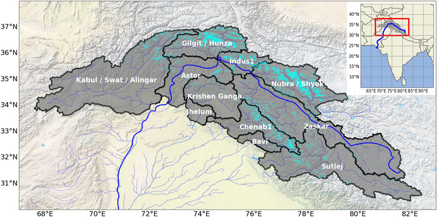
FIGURE 1. The upper Indus Basin (dark gray shading; Wijngaard et al., 2017) divided into the 11 subbasins used in this study (bold black polygon outlines; Immerzeel et al., 2020), shown with glaciers (cyan; RGI Consortium, 2017) and river tributaries (blue; FAO, 2021) to the main stem of the Indus (bold blue; Alexander, 2021). This map has a WGS84 projection. Map baselayer from ESRI with digital layer from National Geographic (2011).

Within the UIB of Wijngaard et al. (2017), we followed the subbasin delineations of the HydroSHEDS-derived product used in Immerzeel et al. (2020). We followed the FAO’s basin aggregations, such as the Gilgit and Hunza into a single “Gilgit/Hunza” subbasin, and we use the naming conventions of the FAO product in this manuscript. However, we recognize that many basins have alternate names and/or spellings. In the scientific literature, counts for subbasins within the UIB range from 5 (Ahmed et al., 2014) to 13 (Dahri et al., 2016). Following the FAO product as we do, there are 11 subbasins, which vary in size, glaciated area, and number of debris-covered glaciers, as summarized in Table 1. The three northernmost basins (Gilgit/Hunza, Indus1, and Nubra/Shyok) fall in the Karakoram Mountain Range, the Kabul/Swat/Alingar in the Hindu Kush, and the remaining seven in the Western Himalaya. The subbasins are shown labeled and superimposed on a UIB-wide map with glaciers and tributaries in Figure 1, and glaciers’ subbasins were defined as the basin in which they terminate.

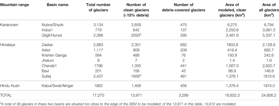
TABLE 1. Inventory of glaciers in the Upper Indus Basin and the area of those modeled (Kraaijenbrink et al., 2017; RGI Consortium, 2017; Scherler et al., 2018).

Meteorological Inputs

The High Asia Refined Analysis (HAR; Maussion et al., 2014) is a gridded atmospheric data product generated by dynamical downscaling of the Global Forecasting System data using the Weather Research and Forecasting model. It provides hourly atmospheric data at 30 km resolution for Central Asia and at 10 km for the area surrounding the data-sparse Tibetan Plateau, including the UIB. We use the 10 km resolution HAR version 1, which includes full calendar years 2001–2013. The model described in the subsequent subsection requires the following inputs from HAR: incoming radiative fluxes at the surface, 2 m air temperature, total precipitation, surface pressure, 2 m relative humidity, emissivity, and 10 m windspeed. We imposed a precipitation cutoff for drizzle at 0.25 mm per day, consistent with instrument limits on measurement (following, e.g., Riley et al., 2021).

The model is driven by meteorological input from HAR and additional variables derived from them that are necessary to calculate the turbulent and outgoing longwave fluxes (e.g., surface saturation vapor pressure). We elected to use HAR for three reasons: first, it has high temporal and spatial resolution and, thus, captures topography better than most other publicly available products. Second, HAR includes all the variables required to force our glacier surface energy and mass balance model. Finally, its validation across High Mountain Asia has been the subject of an extensive set of prior studies (Maussion et al., 2014; Mölg et al., 2014; Pritchard et al., 2019; Yoon et al., 2019). Although using HAR—or, in fact, any gridded product or even automated weather station network in complex terrain—has significant limitations, these validation studies suggest that use of HAR is justified. They show that HAR precipitation seasonality is well-represented, and precipitation is generally consistent with observed values of runoff.

HAR temperatures match observations well when considered daily and hourly but do show a cold bias in winter over the Tibetan Plateau. Biases vary seasonally, with an underestimation of diurnal temperature ranges in spring, early summer, and autumn, times when humidity biases are observed: overestimation of specific humidity in winter and relative humidity in winter, spring, and autumn. The cold temperature bias reduces in summer, along with the high bias in relative humidity. The HAR summer is characterized by underestimation of longwave and overestimation of shortwave radiation, which are results of too-low cloud cover in HAR. While temperature shows seasonal biases (Pritchard et al., 2019), HAR precipitation shows seasonality and spatial patterns consistent with an observation data set of 31 rain gauges on the Tibetan Plateau complemented by the gauge-calibrated estimates of the Tropical Rainfall Measurement Mission (Maussion et al., 2014). Finally, there have been energy balance studies specifically using HAR on glaciers. The most directly relevant is that of (Mölg et al., 2014), in which HAR was input to a full energy and surface mass balance model for Zhadang Glacier in the central Tibetan Plateau (Mölg et al., 2014) used HAR only—without bias correcting or validating individual energy balance inputs—and found good agreement when compared to forcing the same glacier with nearby AWS data. Although a precipitation scaling factor was used to achieve observed mass balances in the Tibetan Plateau, the work of (Mölg et al., 2014) does illustrate the utility of our approach.

HAR’s strength lies in spatial patterns and tendencies so it is well suited to our regional research question. We do not assert that the HAR product represents reality or is free from biases (summarized above) but use it in this study as the assumed climate for the purpose of our investigation.

Input variables from HAR are either assumed constant across the glacier or adjusted for glacier-wide application, following Johnson and Rupper (2020). For example, the HAR wind speed is scaled from 10 to 2 m height (following, e.g., Oke, 1987; Stull, 1988) and then assumed uniform over the entire glacier surface. Both incoming shortwave and incoming longwave radiation are distributed over the glacier based on physical variables. Shortwave is adjusted via glacier slope, glacier aspect, and sun position following Reda and Andreas (2004), and incoming longwave is distributed using an effective emissivity (Braithwaite and Olesen, 1990). These methods of distributing incoming radiation have been used and validated in other regions of the world (e.g., Arnold et al., 1996; Hock and Holmgren, 2005; Wallace and Hobbs, 2006; Ebrahimi and Marshall, 2015; Johnson and Rupper, 2020). We note that the standard assumption of logarithmic wind speed profiles cannot account for katabatic winds. However, not simulating katabatic winds has an impact on the latent heat flux that is at least compensated for by an overestimation of temperature.

Three inputs’ values across a glacier surface are determined by adjusting for the glacier-HAR elevation difference. First, the air pressure, used to calculate turbulent fluxes, is recalculated every timestep from the HAR gridcell elevation to give air pressure at the glacier surface elevation. Second, air temperatures are adjusted using day-of-the-year lapse rates calculated from the 3 × 3 matrix of mean daily temperatures of HAR gridcells centered over the modeled glacier. We calculate the daily climatological lapse rates; thus, the lapse rates are the same for a given date in each year of the model run and are used to scale temperature from the elevation of a glacier’s HAR gridcell to its surface. Third, we updated the Johnson and Rupper (2020) model to include a precipitation gradient, reflecting the well-known general trend of precipitation increase with elevation (e.g., Winiger et al., 2005; Hewitt, 2014; Pritchard et al., 2019). The change in precipitation with elevation is computed by subbasin and is detailed in the subsequent section.

Surface Energy and Mass Balance Model

We use the Surface Energy and Mass Balance Model (SEBM) of Johnson and Rupper (2020), here run hourly at a resolution of 90 m over glacier surfaces, to simulate and quantify melt from snow and ice in the glacier system. Here, we give only a brief overview and highlight adaptations made for this study. We refer the reader to Johnson and Rupper (2020) for model details.

The net energy, Q_net, is the sum of the surface energy fluxes (Eq. 1):

SW is shortwave (solar) radiative flux, LW is longwave radiative flux, H and LE are the sensible and latent heat terms of the turbulent energy flux, Q_P is energy carried by liquid precipitation, and Q_C is the conductive heat flux between the glacier surface and glacier body. While Q_P is commonly neglected in SEBMs (e.g., Wagnon et al., 2003; Mölg and Hardy, 2004), it is included here for completeness. We neglect refreeze, and the only ground flux accounted for is the conductive one: Qc = K_s (T₂—T_s)/d_s, where K_s is the thermal conductivity of the surface layer computed from the layer’s density using the formula of Van Dusen (1929).

An important determiner of the shortwave radiation balance is the surface albedo which, following the methods of Johnson and Rupper (2020), is calculated as a function of the composition of the surface (snow, firn, or ice; values in Appendix Table A1), snow depth, and time since the last snowfall. When the air temperature is equal to or less than the precipitation phase transition threshold (Appendix Table A1), precipitation falls as snow and resets the albedo of the surface to that of fresh snow.

The net surface energy flux controls the evolution of glacier surface temperature such that a change in surface temperature is: $\Delta T_s=\frac{Q_{net}}{c{\rho }_s{d}_s}dt$, where c is the specific heat capacity of ice (= 2097 J kg⁻¹ K⁻¹), ${\rho }_s$ is the surface density computed as a weighted average of the ice and snow contents in the surface layer (Appendix Table A1), and $d_s$ is the thickness of the surface layer (22 cm, after Arnold et al., 2006).

The model is a three-layer model, requiring temperature at the surface, the near-surface (22 cm depth in the glacier), and the glacier body (10 m). The model domain ranges from the surface to a depth of 10 m, and the composition of that 10 m evolves over time as snow and ice accumulate, sublimate, and melt. The model prognoses the evolving temperatures at the surface (T_s) and 22 cm depth (T₂), but the temperature at 10 m depth (T_b) is assumed constant and equivalent to the long-term mean air temperature (Paterson, 1994). The temperature in the second layer changes only by conduction (i.e., only when there is a temperature gradient).

The model calculates conduction through ice, snow, or a combination of the two—but not debris. Thus, we limit our study to the 81% of UIB glaciers (comprising 76% of the glacierized area) that are “clean” glaciers, defined here as glaciers whose areas are less than 15% covered by debris. Debris cover information for 17,252 of the 17,270 glaciers in the UIB (Table 1) is from Scherler et al. (2018), given by the Landsat eight bands 4:6 ratio algorithm of Hall et al. (1987). For 18 glaciers with incomplete attributes in the RGI, we use glacier area from Shean et al. (2020) and debris cover from Kraaijenbrink et al. (2017).

The surface temperature, when calculated as positive, determines the energy available for melt; physically, when energy is present to raise the surface temperature, that energy is absorbed in the endothermic melting of ice such that the actual surface temperature never exceeds 0°C. Note that warming the surface temperature to the melting point requires energy; however, it is only when the calculated surface temperature exceeds 0°C that energy is available for melt (Eq. 3).

Other significant changes from the Johnson and Rupper (2020) model include the introduction of a precipitation gradient that is consistent with HAR and calculated separately for each subbasin. Precipitation increases with elevation as a function of the amount of precipitation (Eq. 4):

where $\overline{P_{HAR}}=p_1{h}_{gl}+p_2$ is the hourly average precipitation (mm h⁻¹) during hours when it precipitates. p₁ and p₂ are, respectively, the slope and y-axis intercept of the robust linear bisquare regression of elevation, limited to the range occupied by glaciers, vs. average hourly precipitation when precipitation is non-zero. Eq. 4 shows that the precipitation on the glacier (P in m) is given by the closest HAR gridcell’s precipitation (in m) adjusted by the difference in elevation (h in m) multiplied by the share of the $\overline{P_{HAR}}$ that falls during the timestep and the lapse rate for the year (p₁, in mm h⁻¹). While precipitation generally increases with elevation, precipitation does decrease in some regions above a certain elevation (e.g., Immerzeel et al., 2012; Hewitt, 2014). Limited observations and 10 km HAR resolution preclude identifying those transitions in this study; there are multiple approaches to and significant uncertainties associated with downscaling precipitation in complex terrain. The effects of precipitation uncertainty are discussed in Uncertainty.

The revised model also includes a stipulation that the stability correction be applied only with the Richardson number (R_b) > 0 and wind speed (U) > 1 m s⁻¹ (Anderson et al., 2010) to accommodate a range of glacier surface temperatures and to prevent unreasonable values at very low wind speeds. The model undergoes a spin-up of 1 year, which is sufficient to establish a depth for the snowpack. Finally, we introduced a correction for large, persistent surface temperature outliers that deviate unphysically due to a combination of forcing variables. These outliers are infrequent and isolated rather than pervasive: though ∼95% of glaciers have extreme outliers, the outliers occur on average in 0.17% of the timesteps. Accordingly, we reset the non-physical, outlying temperature values that vacillate more than 15°C from the previous (hourly) time step’s temperature. Outlying values are set equal to the average surface temperature over the previous 24 h, a more reasonable value; this ensures results within physical reality for the whole time series.

We ran the model at 90 m spatial resolution, having degraded spatial resolution from the 30 m ASTER GDEM V3 to improve run time, and at 1-h time steps over the HAR calendar years 2001–2013. Glacier shapes were given by RGI 6, and glacier mass balance is accumulation less melt and sublimation. Figure 2 shows all three mass balance components in a stacked bar graph, by subbasin. Because evaporation comes from meltwater, we do not double count it in the mass balance calculation. We assume all melt goes to runoff in the model and that, therefore, modeled melt is equivalent to modeled runoff. Additionally, note that, because the Jhelum subbasin includes so few glaciers, we include Jhelum’s glaciers with the Krishen Ganga subbasin, and we report model runs and results over 10 subbasins, rather than 11 (Table 2).

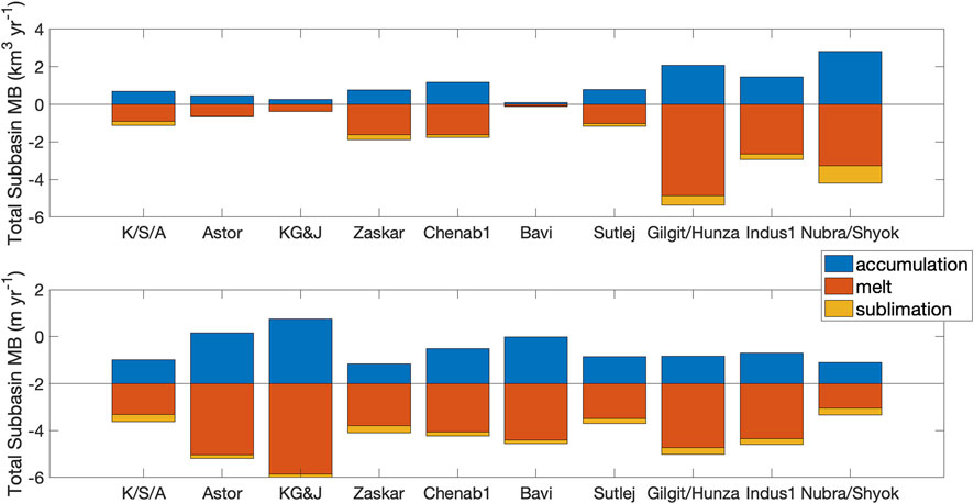
FIGURE 2. The volumetric components of each subbasin’s annual average (2001–2013) clean glacier mass balance (MB), total (upper panel) and normalized for glacier area (lower panel). Melt (red) is the dominant mass balance term, with accumulation (blue) being less and sublimation (yellow) only a small part of the budget. Krishen Ganga and Jhelum are combined into a single basin (KG&J), and K/S/A is Kabul/Swat/Alingar.

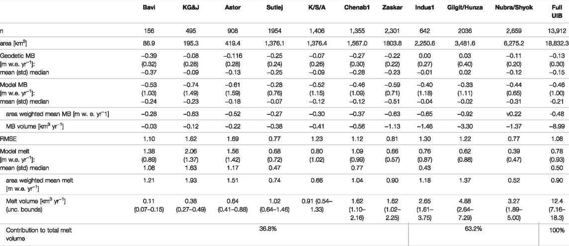
TABLE 2. Results of the surface energy and mass balance model run over all subbasins of the Upper Indus Basin 2001–2013, with geodetic mass balance (MB) from 2001–2018 (Shean et al., 2020). Subbasins are ordered by increasing area to match the order in Figure 5. The average MB and melt are given, as well as corresponding melt volumes and area-weighted means. The RMSE is calculated by comparing a subbasin’s individual glaciers’ modeled MBs with their geodetic MBs. The percent contribution to total melt volume is provided for the northern subbasins and southern subbasins to illustrate the dominance of the northern regions on melt volume. Note that Krishen Ganga and Jhelum are combined into a single basin (KG&J) for the modeling. K/S/A is Kabul/Swat/Alingar.

Calibration

We calibrated the model with 2000–2018 geodetic mass balance data from Shean et al. (2020), which was mostly calculated from ASTER imagery. Forcing the model with 2001–2013 HAR output but calibrating to a longer time range is not ideal, as it can introduce additional uncertainty. However, this was the most complete observational dataset for the region at the time the calibration and validation were completed, and, importantly, it includes smaller glaciers. The timeframe differences between modeled and observed mass balance are unlikely to have significant impacts on the results, as discussed further in Uncertainty. We formed a calibration sample of n = 323 glaciers and extrapolated the calibration parameter to all UIB glaciers; calibrating all would have introduced a significant computational burden and, more importantly, would not have been calibrating the variable of interest, melt. While close agreement between modeled and geodetic mass balance values across the entire study area may have improved the certainty of our melt results, calibrating the mass balance as a whole would not necessarily improve certainty in its components (melt, accumulation, sublimation). Unfortunately, measurements of melt are not available, and myriad combinations of melt, accumulation, and sublimation values can sum to the same value of mass balance. Given that it is not possible to calibrate the melt component of mass balance separately, that calibrating all UIB glaciers would not necessarily improve the certainty in our melt result, and that calibrating all glaciers would have presented a significant computational burden, we opted for minimal calibration to avoid over-calibration of our results and artificial inflation of their reliability. To select the calibration sample, we started with 30 glaciers per basin that were spatially distributed and that had distributions of elevation, slope, aspect, and area closely matching the distributions of those characteristics for all glaciers in that basin. Twenty-three additional glaciers filled spatial gaps and ensured representation of all climate settings. The elevations of the 323 sample glaciers are representative of the glacier elevation range for the broader UIB population (n = 13,912) minus its outliers.

Precipitation is a convenient and reasonable parameter to adjust given its coarse resolution and low accuracy in climate data (Rounce et al., 2020a), particularly in the UIB (Dahri et al., 2016) and other parts of High Mountain Asia (e.g., Wortmann et al., 2018). Thus, while multiple calibration methods exist (Ismail et al., 2020), we chose to reduce the model-measurement bias through a precipitation correction factor (PCF), which was the constant, annual amount by which the total precipitation magnitude (2001–2013) was adjusted from the downscaled HAR precipitation. The PCF value was determined by iteration until modelled mass balance was within 10% of the geodetic mass balance, resulting in one PCF for each of the 323 calibration sample glaciers. The PCF is not a precipitation-bias correction as it effectively incorporated all uncertainty—including SEMB model biases, HAR biases, and downscaling biases—into a single parameter. The 323 PCFs, all of whose values are within physically reasonable bounds, were applied to the 13,912-glacier population by taking the average of PCFs for all sample glaciers within a 20 km radius or, if there were fewer than 10 in that radius, the 10 closest sample glaciers (gives UIB-wide PCF $\mu = -0.68$ and $\sigma =0.20$). This combination, out of nine algorithms identified a priori and shown in Supplementary Table S1, minimized the amount that the PCFs calculated by local averaging varied from the calibrated PCFs for the 323 subset glaciers.

The way that the calibration was applied minimizes the impact of model over-fit: the 323 calibrated PCFs were not input directly to the model. Rather, they were used to calculate every glacier’s individual PCF such that even the 323 glaciers in the calibration subset were modeled with PCF values calculated using the algorithm above. We calibrated an independent set of glaciers (n = 95) spatially distributed across the UIB to confirm that the choice of glaciers for calibration did not affect the results (Supplementary Figure S2B).

We performed 10-fold cross-validation to determine any bias introduced by our local averaging method to estimate PCFs for all glaciers in the UIB. Results of this cross-validation showed minimal systemic bias (μ = 0.02 m w.e. yr⁻¹, Supplementary Figure S2A), supporting our use of this method. The variability in calculated biases for the 10-fold samples ($\sigma$ = 0.1 m w.e. yr⁻¹) shows a minor sensitivity to the exact choice of calibration glacier subset. This sensitivity, however, is likely a reflection of the careful selection of the full training data set (n = 323) to be regionally and geomorphically representative, a characteristic the individual cross-validation subsets lack. The k-fold cross-validation, then, confirms the lack of any significant bias introduced either by the local averaging method for PCF estimation or by the specific glaciers used for calibration.

Uncertainty Assessment

Once calibrated, the model calculates energy and mass fluxes hourly over the surface of each glacier for the duration of the HAR forcing. Totaling the mass balance components (with melt being our focus) and aggregating by subbasin demonstrates differences in each basin’s glacial response to meteorological forcing given by HAR. Calibration is one of two sources of uncertainty that we quantified and applied to the model’s calculation of glacier melt. While the model-measured mass balance bias provided a mass balance uncertainty, it was important not to apply this mass balance uncertainty directly to the melt results because melt is not necessarily off if the mass balance is off (and vice versa). While melt and mass balance uncertainties likely have some relation, they are rarely equivalent.

For glaciers whose mass balance bias is small, but still more than 10%, the uncertainty is assumed to result solely from model parameterization. When mass balance varies greatly from the geodetic mass balance, error stems from calibration-related uncertainty superimposed upon that from parameter choice. We assume that when the bias is due to both, melt uncertainty is a linear function of mass balance. We assume a linear relationship given the absence of a known relation combined with the likelihood that there is generally some relationship between melt uncertainty and mass balance bias. We acknowledge this approach is subjective but use it as a semi-quantitative approach to approaching uncertainties.

To determine the thresholds for the different categories of uncertainty and to quantify melt uncertainty, we ran model tests of 12 glaciers with different parameter and PCF inputs, as described in the subsequent subsections and Supplementary Material. The 12 glaciers were selected because they spanned all subbasins and represented the large range of glacier sizes in the UIB: half were large outliers in a distribution of glacier areas (with outlier defined using the medcouple-based definition of Hubert and Vandervieren, 2008). Modeling the 12 glaciers in the test set yielded quantification of model sensitivity to both the input parameters and the calibration through the following approaches. We apply the melt uncertainty relationships derived from the 12 glaciers to all glaciers, by subbasin, to compute uncertainty in our results.

Melt Uncertainty From Model Parameter Values

Of the parameters used in the SEBM (see Appendix Table A1), any could potentially factor into model uncertainty. However, the ten in Table 3 stand out as relatively less certain and/or more likely to elicit model sensitivity (Braithwaite, 1995; Moore, 1983; Klok and Oerlemans, 2004; Immerzeel et al., 2014; Shea et al., 2015; Giese et al., 2020; Johnson and Rupper, 2020). The albedos of bare ice and fresh snow directly affect the absorption of energy by the surface, while the temperature lapse rate and temperature at which precipitation phase transitions affect whether precipitation falls as rain or snow. This, in turn, controls the surface albedo and the accumulation component of the modelled mass balance. We also tested sensitivity to the six roughness lengths—three each for snow and ice—which are highly variable and difficult to measure directly (Smith, 2014). Roughness lengths are the height above the surface at which the surface itself no longer affects the variable in question: momentum (i.e., wind speed), temperature, or water vapor.

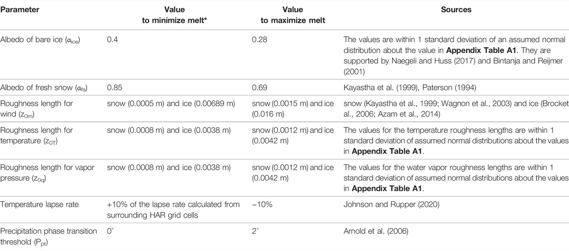
TABLE 3. Values for the 10 parameters used in the uncertainty analysis. See Appendix Table A1 for the control values and their sources.

There were three sets of parameters for the uncertainty analysis: the original ones (Appendix Table A1 or, for lapse rate, the model’s calculated value) and ones specified to minimize and maximize melt (Table 3). For the 12 glaciers, calibration to within 10% of the geodetic mass balance under three parameter sets gave a range of melt variation (i.e., uncertainty) due solely to the model parameters.

Melt Uncertainty From Calibration

After obtaining the mass balances (MBs) in the previous section that were within 10% of the geodetic values, we altered each glacier’s PCF by one standard deviation of the calibration subset’s PCFs (n = 323 glaciers) under each of the three parameter sets. This yielded probable ranges of melt and mass balance due to applying the 323 PCFs to all clean glaciers in the UIB. Because applying the PCF did not include any glacier-specific weighting and was instead the mean of PCFs for the nearby glaciers in the calibration sample, we could perturb all glaciers in the uncertainty analysis with the same change in PCF (here, $\pm \sigma$). This perturbation revealed that the precipitation adjustment (i.e., PCF) affects the components of mass balance equally; for the 12 test glaciers, the melt response range was 49.85% of the full MB response range (see Supplementary Figure S4).

Results

Error/Uncertainty

We divide our model results into three categories based on how well the model performs, and we use the 12-glacier set to quantify melt uncertainties in each (a more detailed version of what follows, including a more detailed version of the figure, can be found in the Supplementary Material). These were 1) model (parameter) uncertainty only; 2) model + calibration uncertainty; and 3) model + greater calibration uncertainty for glaciers whose mass balance deviation from measured values was classified as an outlier (details are provided in Figure 3 and the Supplementary Material). Calibration was the biggest source of melt uncertainty in our results. Calibration adds uncertainty on top of the relatively small amount from model parameters, but the two are not merely additive because parameters may affect model sensitivity to calibration.

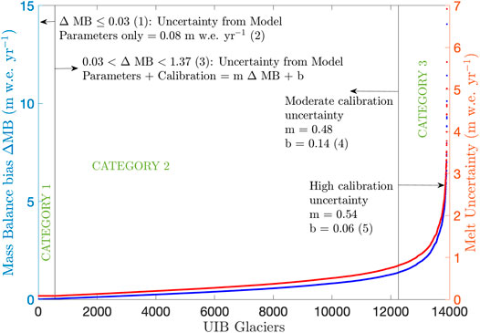
FIGURE 3. Melt uncertainty (solid red line) of Upper Indus Basin glaciers depicted as a function of the model-measured mass balance bias (“ΔMB,” solid blue line), based on sensitivity analysis of a 12-glacier set that represented Upper Indus Basin subbasins and glacier sizes. The vertical lines show where the MB difference is 0.03 and 1.37 m w.e. yr⁻¹. At these values the uncertainty category changes from 1 to 2 and from 2 to 3, respectively. A detailed derivation of all values in the figure is given in the Supplementary Material.

The melt uncertainty analysis performed here is likely a reasonable first-order estimate and is, therefore, useful for assessing the relative difference in and sources of melt uncertainties across the UIB. In the subsequent sections, we present and focus on our results, which are robust given the uncertainties in modeled melt.

Melt

The SEBM applied to the UIB’s clean glaciers elucidates regional patterns in melt energy and its components. We emphasize again here that the significant paucity in observations precludes a complete calibration and validation of melt in this region. Thus, these results should be viewed as a theoretical assessment of plausible variations in melt, rather than a definitive quantification of melt. Within this theoretical framework, the amount of melt on any glacier is a complex function of the glacier’s geomorphic characteristics, surface properties, and climate. Across the UIB, glaciers melt for different proportions of the 13-years model run (Figure 4A). Days with melt correlate with mean daily energy available for melt (Figure 4B), which tends to increase towards the southwest. The average daily melt energy is reflected in the area-weighted mean melt of each subbasin (Table 2). Melt has a stronger correlation (R² = 0.35) with elevation than any other component of the mass balance or even the mass balance itself. The glaciers with high melt energy tend to be those located at lower elevations, but, with an R² = 0.35, elevation is only a weak predictor of melt.

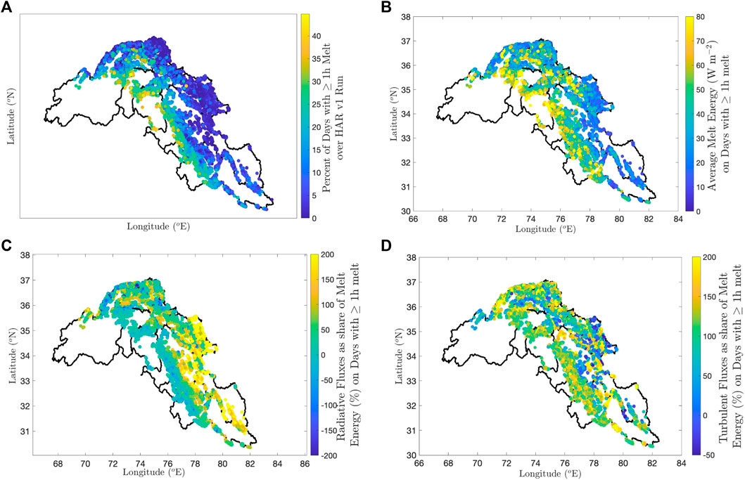
FIGURE 4. Map of the Upper Indus Basin showing (A) percent of days with at least 1 hour of melt, and, on those days, (B) average melt energy. (C,D) show the percents of that average daily melt energy comprised of radiative and turbulent fluxes, respectively. The component percents add to 100 and may individually have values less than 0 or exceeding 100. For scale, refer to Figure 1. Note that these figures are not projected into a coordinate system but rather show the Upper Indus Basin with linear spacing of latitude and longitude on the axes. The model runs span 2001–2013.

Figures 4C,D show the relative contributions of daily mean radiative and turbulent fluxes to the daily mean melt energy on days with melt. We do not show energy associated with precipitation and subsurface conduction because of their relatively small contributions to the overall net energy. Because energy fluxes are additive (Eq. 1), the percents can exceed 100% (see also Fitzpatrick et al., 2017). Radiative fluxes seem to dominate the melt energy in the northeastern subbasins Nubra/Shyok and Zaskar, whereas turbulent fluxes dominate in the west (Kabul/Swat/Alingar, Gilgit/Hunza) and south (Chenab1, Bavi, Sutlej). The three central basins seem to be a mix, with no clear dominant contributor to the melt signal. Because turbulent heat flux equations perform poorly for sublimation (Rupper and Roe, 2008), with many of the assumptions made in the calculation of sublimation violated in extreme terrain (Stigter et al., 2018), the flux composition of glaciers whose mass balance is dominated by sublimation—mostly concentrated on the northern boundary of Kabul/Swat/Alingar and Gilgit/Hunza and the eastern part of Nubra/Shyok—is less certain. The sublimation-dominated glaciers are a minority, though, and they do not change the broad basin-wide trends in melt energy components.

While dry, arid conditions dominate across the northeastern part of the UIB (Joshi et al., 2005; Gascoin, 2021), we do not see turbulent fluxes dominate in this area as Gascoin (2021) finds for snow because turbulent fluxes can dominate snow mass loss while radiative fluxes dominate the ice mass loss. Compared to snow, glacier ice extends to lower elevations throughout the summer (experiencing warmer temperatures and, thus, more longwave fluxes); additionally, it is darker than snow for longer periods of time and, thus, absorbs more shortwave radiation. Melt is 8.5 times more efficient than sublimation; therefore, radiatively-driven melt can dominate the mass balances on a glacier while sublimation dominates mass changes in higher elevation snowpack.

Spatial patterns in melt and its components are important for understanding dominant controls and regional gradients. From the perspective of water resources, though, it is necessary to compare integrated, subbasin-wide glacier melt. Basins that have more glaciers to begin with are going to be able to produce more melt. However, the relationship of melt volume with glacierized area for each subbasin is not a simple linear relationship (Figure 5).

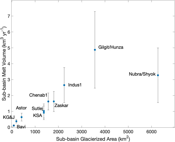
FIGURE 5. Annual average glacier melt volume (2001–2013) from clean glaciers, aggregated by subbasin, for the Upper Indus Basin, with uncertainty bounds computed via a 12-glacier test set. Krishen Ganga and Jhelum are combined into a single basin (KG&J), and K/S/A is Kabul/Swat/Alingar.

Mass Balance

Although this study aimed to compute and explore patterns in glacier melt, glacier mass balance is the sole metric for which model output can be evaluated against measured values (e.g., in situ, geodetic) across this vast region. Unfortunately, in situ mass balance observations are extremely limited in the region. Still, existing ones provide some information on temporal variance and spatial distribution of mass balance on glaciers. Two of the 13,912 modeled glaciers are included in the World Glacier Monitoring Service (WGMS) database and cover shorter time periods than the model does (2001–2013): Chhota Shigri (2003–2013) and Patsio (2011–2013) glaciers (WGMS, 2021). Figure 6 shows modeled mass balance and available observations for these two glaciers. The 2009–2013 portion of the record for Chhota Shigri matches the model output well, while there appears to be a positive bias in the model for glacier-wide values in the early part of the record. During part of that time, 2003–2006, elevation-distributed annual mass balance values are available, and Johnson and Rupper (2020) found that these observations fall within the modeled mass balance range (see Johnson and Rupper (2020)’s Figure 3). For Patsio, there are fewer data (only 3 years), and it is difficult to make broad conclusions. Still, we do note that in those years of overlap there is a negative bias in the model. Such year-to-year comparisons have limited utility because we do not expect HAR to capture the specific climate of any given year. Far more telling are comparisons of the mean and range: for Patsio glacier, the 3 years are roughly within the range of the modeled output (but, once again, the number of years is too limited to assess whether the model generally captures the long-term mean or variability). For Chhota Shigri glacier, the model captures some of the variance well but does not capture the most negative years. The observed mean (−0.60 m w.e.) and variance (0.45 m w.e.) are greater in magnitude than the modeled mean (−0.01 m w.e.) and variance (0.12 m w.e.) for the same period. The general biases seen in the model-observations comparisons are similar to those seen when comparing to geodetic mass balance observations.

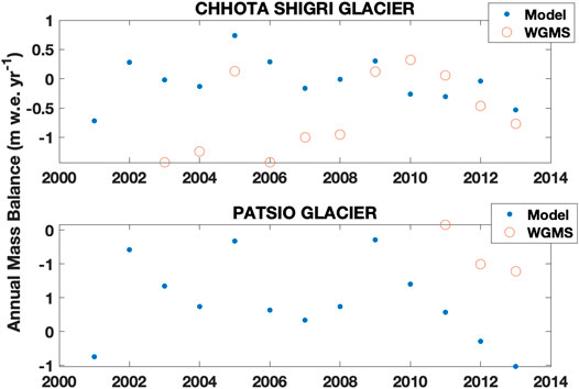
FIGURE 6. Time series of modeled (2001–2013) and measured annual mass balance measurements for Chhota Shigri glacier (2003–2013) and Patsio glacier (2011–2013), the only two glaciers in the UIB that have annual mass balance data in the WGMS database.

The geodetic mass balance data used in this study (Shean et al., 2020) do not directly provide information on temporal variance or mass balance distribution on a glacier, but they do provide a more spatially complete dataset for data-model comparisons. Figure 7 gives a histogram of the modeled and geodetic mass balance values (excluding the modeled values for calibrated glaciers). Salient in this histogram is the long, left tail of the modeled MBs, which appears also as the large MB bias in Figure 3; Supplementary Figure S3 (model-data MB discrepancies can be extremely large). Although, as stated in Calibration, it is not possible to attribute a model-data mismatch to the various MB components specifically, when the model yields a large model-data mismatch, it likely also simulates melt poorly. Uncertainty in melt is calculated as a function of MB bias (see Supplementary Material) to account for this, and the 11.9% of glaciers with large uncertainty (Category 3 in Figure 3; Supplementary Figure S3) have larger uncertainties in their melt and melt volumes than those with lesser MB biases.

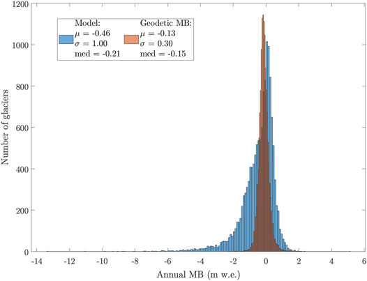
FIGURE 7. A histogram comparison of modeled annual average mass balance values and geodetic ones from Shean et al. (2020) for all glaciers in the Upper Indus Basin, excluding the 323 used to calibrate the precipitation correction factors. Basic comparative statistics are displayed in the legend.

The significantly different variances between the modeled and geodetic MB values are evident in the long left tail described above—and also in both the standard deviations and the medians’ departure from the means. The model and geodetic mass balance data distributions also vary in skewness (with values of −2.20 and 0.88, respectively). These differences in variance and skewness are present at the subbasin level, as well. The glacier-by-glacier RMSE by subbasin (Table 2) indicates that the model performs best for the Nubra/Shyok and Sutlej subbasins (both have RMSE = 0.77) and worst for Astor (RMSE = 1.69) and the combined Krishen Ganga and Jhelum (RMSE = 1.62). Mass balance does not show a clear correlation with area or other individual characteristics (e.g., aspect, slope, length, hypsometric index). The modeled MB tends to deviate from the geodetic values most for lower elevation glaciers, but we did not find a strong linear correlation between elevation and the geodetic MB–model MB difference.

Of the four lowest subbasin-wide mean modeled MBs, three are in the Karakoram. Mass balances tend to be small in the Karakoram (hence, the “Karakoram Anomaly”), but, as discussed above, a small mass balance does not imply a small melt because mass balance can still be small with a large mass turnover. The melt volumes from the three Karakoram subbasins are the greatest of all UIB subbasins. In these subbasins, glaciers are large, and there are large areas over which melt can occur. All three Karakoram subbasins show skews in the distribution of their glacier areas, with many small glaciers. A relatively small number of large glaciers contribute the majority of melt. In Table 2, it is clear that mean melt (in m w.e. yr⁻¹) is not notably large in the Karakoram subbasins. It is greater than the median melt, reinforcing that the melt for the largest glaciers is higher than the mean melt for all glaciers. The large, glaciated areas more than compensate for the low subbasin-wide average melt values since mass balance in m w.e. is multiplied by area to get volumetric mass balance.

Discussion

Variance

Modeled mass balance shows much more variance than the geodetic MBs for the UIB as a whole (Figure 7) and for each subbasin. Notably, there is a left skew in the model MBs that is absent in the measurements; this is reflected graphically and in the model MB mean and median values, which are lower than the corresponding values for the geodetic MB. The mode of the modeled values is greater, again reflecting the long left tail that is comprised of relatively fewer glaciers (more glaciers have greater modeled MBs). The likely culprit for the larger variance and skewness of the modeled values is the way that the calibrated PCFs are applied to all UIB glaciers (described in Calibration; see also Uncertainty below). Three factors likely impact variance when it comes to the PCF. First, we averaged local PCFs without weighting by distance or geomorphic similarity to the modeled glacier. Second, we calibrated total annual precipitation, although adjusting precipitation when it is rain vs. snow has different impacts on glacier mass balance. Finally, calibration coefficients are unlikely to be constant across time. This is especially true because the process of calibration encapsulates all biases that make the model differ from measurements—not just precipitation—into the “precipitation” correction factor. Many factors are wrapped up in the calibration and, therefore, impact the variance. These other factors inherently represented in the PCF include biases in the HAR climate variables, how well the model physics are represented with a 1-h model timestep, interactions of model parameters, effects of neglecting melt refreeze, and the simplified treatment of subsurface heat.

Further, geodetic mass balance and model output mass balance may not be truly identical quantities. The geodetic mass balance data are calculated by applying a single density of ρ = 850 kg m⁻³ (Shean et al., 2020) to a remote-sensing-based glacier volume change, whereas the model computes mass balance through explicitly representing melt, sublimation, and accumulation and accounting for the differences in ice and snow density. The constant density assumption in geodetic MB may underrepresent variability and contribute to the lower variance in the MB observations. Another potential contributor to the variation difference is that the model does not account for SW shading or topographic effects on emitted LW. The modeled MBs in the left tail of the right-skewed distribution shown in Figure 7 are for glaciers at low elevations, and the variance of the model is greater than that of the measurements, even when excluding these outliers.

The UIB’s Glaciers

Modeled melt for the glaciers in Nubra/Shyok is proportionally less than that for glaciers in Gilgit/Hunza, even though they collectively have 1.8 times the glacierized area. The Kabul/Swat/Alingar has essentially the same glacierized area as Sutlej, and yet the glaciers in the Sutlej subbasin produce 12% more modeled melt volume. Conversely, Chenab1 and Zaskar produce the same amount of modeled melt, but Zaskar’s glaciated area is 15% greater. The area weighted mean melt (Table 2), generally equal to the total melt volume in a basin normalized by the total glacier area, corroborates these statements and highlights that the Nubra/Shyok has the lowest area-normalized melt rate of any subbasin. Even when the calculated uncertainty is considered, melt does not scale directly with glacierized area.

The basins show different responses to the HAR meteorological forcing due to both spatial variations in the meteorology and the basins’ considerable variations in size and the glaciers they contain. The majority of modeled melt comes from a relatively small number of glaciers, which is a result of having a range of glacier sizes in each basin. For example, 60% of the glacier melt volume in the Gilgit/Hunza comes from 17.5% of its glaciers, and 60% of the glacier melt volume in the combined Krishen Ganga and Jhelum subbasins is from 34.3% of its glaciers. 80% of the total UIB glacier melt comes from 40% of glaciers (Figure 8).

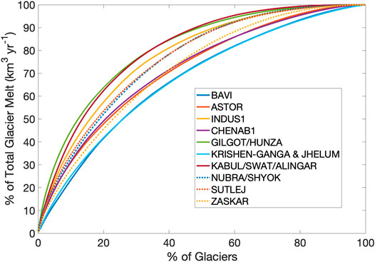
FIGURE 8. Glaciers contributing to annual average melt (2001–2013), by subbasin. If each glacier produced the same amount of melt, there would be a 1:1 line. The logarithmic-shaped curves demonstrate that, by number, a minority of glaciers contribute the majority of melt. Those contributing the most melt are the biggest glaciers.

Hypsometric curves, showing glacier area vs. elevation by 50 m elevation band (RGI Consortium, 2017), provide some insight into why some basins produce more melt water volume than others. Of the three most glaciated basins—in order, Nubra/Shyok, Gilgit/Hunza, and Indus1—the Gilgit/Hunza glaciers melt notably more and are situated at lower elevations, where they experience warmer temperatures. Gilgit/Hunza’s peak elevation in the curve of Figure 9 is 400 m lower than Indus1’s and 450 m lower than Nubra/Shyok’s.

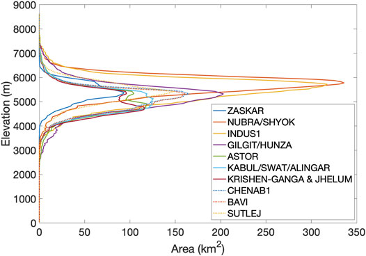
FIGURE 9. Glacier hypsometry by subbasin using the Randolph Glacier Inventory database of area by 50 m elevation band (RGI Consortium, 2017).

Uncertainty

The 12-glacier “uncertainty test set,” which was meant to capture a spread of glacier sizes and regions, allowed us to place the results into the context of the uncertainties. While a full Monte Carlo experiment, or similar, could provide greater detail, the computational requirements of the model precluded such an investigation. Although our subset of 12 glaciers is not exhaustive, it nevertheless served to highlight key sensitivities to model parameters and calibration. Although uncertainties remain large and difficult to quantify at the basin-wide/regional scale, our uncertainty analysis revealed that the SEMB parameters impose smaller uncertainties compared to the calibration (parameter-only uncertainties were found up to a MB bias of only 0.03 m w.e. yr⁻¹). The “uncertainty from calibration” implicitly includes biases in the climate variables and downscaling those variables to scales requisite for distributed glacier models.

Uncertainty from calibration could have potentially been decreased by calibrating all glaciers or making the PCF calculation for an individual glacier more robust through, for example, weighting by elevation or another geomorphic characteristic. The community has highlighted difficulties of applying calibration (e.g., Rounce et al., 2020a; Rounce et al., 2020b). It is essential to strike a balance between calibrating one glacier based on others (which is common practice but introduces errors) and over-calibrating (which would negate the modeling results). The difficulty we found in applying calibration regionally, despite our attempts to circumvent this somewhat by using a PCF calculated from those of multiple nearby glaciers, is similar to previous work on single glaciers (MacDougall and Flowers, 2010; Zolles et al., 2019).

Our approach avoids over-calibrating and is computationally reasonable—but at the expense of greater certainty. While the central tendency of the modeled mass balance is similar to the geodetic mass balance observations, model-data discrepancies can be extremely large. Of the 11.9% of glaciers having a model-geodetic MB bias classified as an outlier (greater than 1.37 m w.e. yr⁻¹ according to the outlier definition of Hubert and Vandervieren, 2008, detailed in the Supplementary Material), 5.9% have biases exceeding 2 m w.e. yr⁻¹ and 2.47% have biases exceeding 3 m w.e. yr⁻¹. Some of these biases average out at the subbasin scale but, given the skew towards negative mass balance bias (Figure 7), there is likely a bias towards overestimating melt in our approach.

Uncertainties in precipitation, though partly mitigated through our choice of precipitation for a calibration parameter, may still affect the model output and results. Achieving accuracy when downscaling precipitation in mountainous regions where it varies greatly over small distances (Lutz et al., 2014) is a challenge, particularly where strong vertical gradients exist (e.g., in the UIB: Hewitt, 2014; Winiger et al., 2005). The model’s precipitation gradient and PCF affect the amount of snow vs. rain. Precipitation phase directly determines surface albedo, subsurface heat flux, and sensible heat flux from rain; therefore, it directly affects a glacier’s surface energy balance, which affects the MB’s ablation term. Solid precipitation comprises the accumulation term of mass balance. Thus, there are two ways for a change in precipitation to impact the MB directly.

An incorrect precipitation directly impacts the energy balance and directly (and indirectly) affects the modeled MB. Importantly, perturbations of the PCF reveal that ∼50% of the mass balance uncertainty is due to melt (Supplementary Figure S4). The difficulty of assessing the precise share of uncertainty driven by precipitation in general provided additional motivation to apply the calibrated correction to precipitation over other variables. Although isolating uncertainty from precipitation is difficult, we do assess overall uncertainty in our results.

Model parameters may change the model’s sensitivity to the PCF. We did not address this specifically and note that the computed bounds shown in Figure 5 do not include this source of uncertainty. However, since the uncertainty bounds were calculated conservatively (see Supplementary Material for calculation details), they may encompass any uncertainty added by this parameter-calibration interaction. Other sources of uncertainty include equifinality, a problem that can be mitigated by calibrating with multiple datasets (Azam et al., 2021), and glacier debris (described below). The model itself does not include glacier dynamics and neglects the radiative effects of dust and black carbon on glacier surfaces. By neglecting dynamics, our mass balance estimates do not include feedbacks associated with elevation change over time (e.g., glaciers thin into warmer climates which amplify melt processes). In addition, surface velocities would advect firn/snow from higher elevations to lower elevations which would affect the areal distribution of snow versus ice seasonally. While these types of dynamic influences are assumed to be small effects over the 13 years of focus in this study, they do introduce additional uncertainties. Coupling a dynamics model to a surface energy balance one, such as done with GloGEMFlo by Zekollari et al. (2019), would be a valuable next step—and is certainly a critical one over longer timescales.

Debris-covered glaciers are an important and complex component of glacierized regions in High Mountain Asia (HMA, e.g., Herreid and Pellicciotti, 2020; Scherler et al., 2018). This study excludes the UIB’s 3,299 debris-covered glaciers, which also contribute to glacier meltwater volume. Thus, our results are limited to clean glacier contributions to meltwater in the UIB. The model also assumes the small areas of debris cover on clean glaciers (up to 15% of total glacier area) are clean ice. In regions where debris exceeds a few cm in thickness, melt rates are likely overestimated in the model. In transition regions between clean ice and debris, where debris is thinner, modeled melt rates are likely underestimated. These two effects offset each other in the modeled melt, though the magnitude of this offset depends on the areal distribution of the debris thickness and is likely variable across the region. Neglecting debris-covered portions of these clean ice glaciers, therefore, introduces additional uncertainty in our model results.

Running the model 2001–2013 but calibrating with geodetic MB data from 2000–2018 introduces uncertainty into the calibration and, thus, results. However, regional aggregations of MB over decades-long ranges points to a wide range of geodetic MBs overlapping in uncertainty bounds for differing decades of coverage (Gardelle et al., 2013; Kääb et al., 2015; Maurer et al., 2019; Shean et al., 2020). In addition, these studies show similar spatial patterns in mass balance across HMA. Therefore, although we would expect greater mass loss in more recent years, we assume that the relative magnitudes and spatial patterns of geodetic MB would remain similar between the different time periods.

Generally, the area-melt relationships hold in the face of these uncertainties for two reasons. First, because uncertainty is calculated in meters of melt, it increases with area, its effect being compounded for very large glaciers and highly glaciated basins. The basins with lower elevation glaciers (more commonly misrepresented by the model) have smaller areas, and, thus, their larger errors don’t compound as much in the melt volume calculation (Figure 5).

Second, we expect the model to have a consistent bias in over- or under-predicting melt. The modeled MBs relative to observations (i.e., geodetic values) shown in Figure 7 for the full UIB have a distribution—with a long tail in negative model MB values—that is present in all subbasins. Such similarity in distributions suggests that biases are consistent between subbasins (i.e., if the model overpredicts in some basins, it likely overpredicts in all). All subbasins have the same systematic bias, and it’s unlikely that the causes of uncertainty shift the model MB in one basin significantly more than in another. Therefore, although Figure 5 shows increasingly large error bounds for more glaciated basins, the relatively greater melt in the Gilgit/Hunza is not likely an artifact of the model.

Conclusion

This study illustrates the utility of mass and energy balance studies for providing perspective on the potential physical drivers of glacier change at regional and global scales. However, the limited nature of observations of glacier and climate variables across the UIB remains a barrier to modeling glacier melt across the region accurately. We acknowledge there are significant uncertainties associated with our model results and, therefore, treat the results as estimates of melt within a purely theoretical framework given HAR climate as the forcing. Within this context, our main findings are:

A) Spatial patterns exist in the dominant contributor to glacier melt. Radiative fluxes dominate the melt signal in the northeastern subbasins (Nubra/Shyok and Zaskar), whereas turbulent fluxes dominate in the western (Kabul/Swat/Alingar, Gilgit/Hunza) and southern (Chenab1, Bavi, Sutlej) ones. The remaining basins have no clear dominant contributor to the melt signal; melt is driven by a mix of turbulent and radiative fluxes.

B) The relationship between glacierized area and melt volume is not 1:1. While basins with more glaciated area have the potential to generate more glacier melt, the extent of glaciers is not a predictor for glacier melt in the UIB. Of the three most glaciated basins (Nubra/Shyok, Gilgit/Hunza, and Indus1), the Gilgit/Hunza glaciers melt notably more (2.64–7.29 km³ yr⁻¹), at least in part due to their lower elevations. After Gilgit/Hunza, Nubra/Shyok (1.89–5.00 km³ yr⁻¹) then Indus1 (1.61–3.75 km³ yr⁻¹) produce the greatest annual volumes of glacier meltwater.

C) Calibration dominates the uncertainty in our results. The selection of model parameters contributes relatively little to overall uncertainty in results. There was only a weak relationship between model performance and glacier elevation, highlighting that not every low-elevation glacier was poorly represented by the model. However, the glaciers for which the model performed poorly—calculating MBs that differed substantially from geodetic ones—tended to be situated at lower elevations.

Glaciers are crucial to maintaining and regulating the flow of the Indus River, which is “dominated by temperature-driven glacier melt during summer” (Lutz et al., 2014). Our study helps elucidate where UIB glaciers melt, a crucial prerequisite for examining changes in when they melt. The timing of glacier melt informs future hydrological projections involving the annual hydrograph (Lutz et al., 2016), extremes (Wijngaard et al., 2017), and the balance of supply with variable demands (Wijngaard et al., 2018; Ciraci et al., 2020). This research on the relative glacier melt contributions of the UIB’s subbasins points to the need for a fully calibrated and validated energy balance model and climate data that can accurately capture the timing, amount, and physical drivers of melt in the region. It also suggests that a complementary understanding of the spatial patterns in water withdrawals is needed. By quantifying water use at a similarly fine spatial resolution, a complete vulnerability assessment for the UIB’s glaciers could be achieved.

Data Availability Statement

The code for the model used and updated in this study can be found at https://github.com/alexandragiese/sebm. All other data come from published sources and are as follows. The glacier outlines and characteristics are available from the Randolph Glacier Inventory (RGI) version 6 (https://www.glims.org/RGI/rgi60_dl.html) with debris cover from Scherler et al. (2018) (https://dataservices.gfz-potsdam.de/panmetaworks/showshort.php?id=escidoc:3473902). For the 18 glaciers with incomplete attributes in the RGI, glacier area comes from the same source as geodetic MB and debris cover is from https://mountainhydrology.org/data-nature-2017. The geodetic MB data are from Shean et al. (2020) (https://github.com/dshean/hma_mb_paper/tree/master/data/mb), and climate variables are from the HAR v1 (https://www.klima.tu-berlin.de/index.php?show=daten_har). The Indus subbasin delineations used follow those of Immerzeel et al. (2009) (https://zenodo.org/record/3521933#.YQ-jtNKjUo), and the ASTER GDEM V3 is available for public download (https://asterweb.jpl.nasa.gov/gdem.asp). Model output is available upon request.

Author Contributions

AG revised and ran the model, analyzed model output, and wrote the manuscript. SR conceived the study and provided guidance on the analysis and manuscript. Guidance using model and HAR data was provided by EJ who consulted on issues and provided feedback throughout the project. DK designed Figure 1 and provided detailed feedback and discussion on the manuscript while in preparation. RF provided project direction, research feedback, and manuscript feedback. All authors reviewed and edited the manuscript.

Funding

This work was supported by the NASA grants awarded to PIs Summer Rupper (NNX16AQ61G and 80NSSC20K1594) and Richard Forster (80NSSC19K1498).

Conflict of Interest

The authors declare that the research was conducted in the absence of any commercial or financial relationships that could be construed as a potential conflict of interest.

Publisher’s Note

All claims expressed in this article are solely those of the authors and do not necessarily represent those of their affiliated organizations, or those of the publisher, the editors, and the reviewers. Any product that may be evaluated in this article, or claim that may be made by its manufacturer, is not guaranteed or endorsed by the publisher

Acknowledgments

Thanks go to Arthur Lutz for guidance on UIB and subbasin delineation. Collin Riley developed the UIB shapefile based on published work and made the UIB glacier mask and glacier number raster from the ASTER DEM. Jim Steenburgh provided data storage and interactive node access at the University of Utah’s Center for High Performance Computing (CHPC). Martin Cuma at CHPC provided guidance on optimizing model run time. Simon Brewer provided perspective and advising on quantifying uncertainty.

Supplementary Material

The Supplementary Material for this article can be found online at: https://www.frontiersin.org/articles/10.3389/feart.2022.767411/full#supplementary-material

APPENDIX

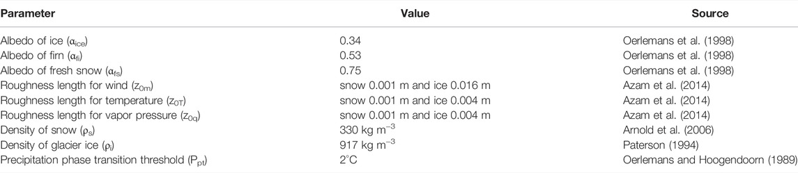
TABLE A1. Parameters used in the model and their values. For a complete list, including constants, see Johnson and Rupper (2020).

References

Ahmed, M. F., Rogers, J. D., and Ismail, E. H. (2014). A Regional Level Preliminary Landslide Susceptibility Study of the Upper Indus River basin. Eur. J. Remote Sensing 47 (1), 343–373. doi:10.5721/eujrs20144721
Akhtar, M., Ahmad, N., and Booij, M. J. (2008). The Impact of Climate Change on the Water Resources of Hindukush–Karakorum–Himalaya Region under Different Glacier Coverage Scenarios. J. Hydrol. 355 (1–4), 148–163. doi:10.1016/j.jhydrol.2008.03.015
Alexander, A. (2021). Indus River (Indus_river_kkl). ArcGIS Online Organization, accessed via WorldMap @ Harvard Community. Available at: https://worldmap.maps.arcgis.com [Accessed August 26, 2021].
Anderson, B., Mackintosh, A., Stumm, D., George, L., Kerr, T., Winter-Billington, A., et al. (2010). Climate Sensitivity of a High-Precipitation Glacier in New Zealand. J. Glaciol. 56 (195), 114–128. doi:10.3189/002214310791190929
Arnold, N. S., Rees, W. G., Hodson, A. J., and Kohler, J. (2006). Topographic Controls on the Surface Energy Balance of a High Arctic valley Glacier. J. Geophys. Res. Earth Surf. 111 (F2). doi:10.1029/2005jf000426
Arnold, N. S., Willis, I. C., Sharp, M. J., Richards, K. S., and Lawson, W. J. (1996). A Distributed Surface Energy-Balance Model for a Small valley Glacier. I. Development and Testing for Haut Glacier D' Arolla, Valais, Switzerland. J. Glaciol. 42 (140), 77–89. doi:10.3189/s0022143000030549
Azam, M. F., Kargel, J. S., Shea, J. M., Nepal, S., Haritashya, U. K., Srivastava, S., et al. (2021). Glaciohydrology of the Himalaya-Karakoram. Science 373 (6557), eabf3668. doi:10.1126/science.abf3668
Azam, M. F., Wagnon, P., Vincent, C., Ramanathan, A., Favier, V., Mandal, A., et al. (2014). Processes Governing the Mass Balance of Chhota Shigri Glacier (Western Himalaya, India) Assessed by point-scale Surface Energy Balance Measurements. The Cryosphere 8 (6), 2195–2217. doi:10.5194/tc-8-2195-2014
Bair, E., Stillinger, T., Rittger, K., and Skiles, M. (2021). COVID-19 Lockdowns Show Reduced Pollution on Snow and Ice in the Indus River Basin. Proc. Natl. Acad. Sci. USA 118 (18), e2101174118. doi:10.1073/pnas.2101174118
Basharat, M., Umair Ali, S., and Azhar, A. H. (2014). Spatial Variation in Irrigation Demand and Supply across Canal Commands in Punjab: A Real Integrated Water Resources Management challenge. Water Policy 16 (2), 397–421. doi:10.2166/wp.2013.060
Bintanja, R., and Reijmer, C. H. (2001). Meteorological Conditions Over Antarctic Blue-Ice Areas And Their Influence On The Local Surface Mass Balance. J. Glaciol. 47, 37–50. doi:10.3189/172756501781832557
Braithwaite, R. J. (1995). Aerodynamic Stability and Turbulent Sensible-Heat Flux over a Melting Ice Surface, the Greenland Ice Sheet. J. Glaciol. 41, 562–571. doi:10.3189/s0022143000034882
Braithwaite, R. J., and Olesen, O. Β. (1990). A Simple Energy-Balance Model to Calculate Ice Ablation at the Margin of the Greenland Ice Sheet. J. Glaciol. 36 (123), 222–228. doi:10.3189/s0022143000009473
Briscoe, J. (2014). The Harvard Water Federalism Project - Process and Substance. Water Policy 16 (S1), 1–10. doi:10.2166/wp.2014.001
Briscoe, W. J., Qamar, U., Contijoch, M., Amir, P., and Blackmore, D. (2005). Pakistan’s Water Economy: Running Dry. The World Bank.
Ciraci, E., Velicogna, I., Grogan, D. S., Proussevitch, A. A., Lammers, R. B., and Yang, Y. C. E. (2020). Interannual Changes of the Upper Indus Basin Hydrological Cycle. American Geophysical Union Fall Meeting. C035-06.
Craig, R., Ruple, J., Tanana, H., and Arrington, C. (2019). Pakistan Water Management—the Legal and Institutional Framework: Lessons Learned and Opportunities for Improvement. U.S. Pakistan Center for Advanced Studies in Water.
Dahri, Z. H., Ludwig, F., Moors, E., Ahmad, B., Khan, A., and Kabat, P. (2016). An Appraisal of Precipitation Distribution in the High-Altitude Catchments of the Indus basin. Sci. Total Environ. 548-549, 289–306. doi:10.1016/j.scitotenv.2016.01.001
Ebrahimi, S., and Marshall, S. J. (2015). Parameterization of Incoming Longwave Radiation at Glacier Sites in the Canadian Rocky Mountains. J. Geophys. Res. Atmos. 120 (24), 12536–12556. doi:10.1002/2015jd023324
FAO (2011a). AQUASTAT Country Profile – Pakistan. Rome, Italy: Food and Agriculture Organization of the United Nations FAO.
FAO (2011b). AQUASTAT Transboundary River Basins – Indus River Basin. Rome, Italy: Food and Agriculture Organization of the United Nations FAO.
FAO (2021). FAO AQUAmaps Global River Data (Major Rivers of the World). Available at: http://www.fao.org/geonetwork/srv/en/main.home [Accessed August 4, 2021].
Farhan, S. B., Zhang, Y., Aziz, A., Haq, M., Gao, H., Naeem, S., et al. (2018a). Calibrating Snow and Glacier Melt Runoff Model by Employing In-Situ Measurements and Satellite Data to Predict Future Melt-Water Flows in High-Altitude basin of North Pakistan. 42nd COSPAR Scientific Assembly 42, A3–A1.
Farhan, S. B., Kainat, M., Shahzad, A., Aziz, A., Kazmi, S. J. H., Shaikh, S., et al. (2018b). Discrimination of Seasonal Snow Cover in Astore Basin, Western Himalaya Using Fuzzy Membership Function of Object-Based Classification. Int. J. Econ. Environ. Geology., 20–25.
Farhan, S. B., Zhang, Y., Ma, Y., Guo, Y., and Ma, N. (2014). Hydrological Regimes under the Conjunction of westerly and Monsoon Climates: A Case Investigation in the Astore Basin, Northwestern Himalaya. Clim. Dyn. 44 (11–12), 3015–3032. doi:10.1007/s00382-014-2409-9
Fitzpatrick, N., Radić, V., and Menounos, B. (2017). Surface Energy Balance Closure and Turbulent Flux Parameterization on a Mid-Latitude Mountain Glacier, Purcell Mountains, Canada. Front. Earth Sci. 5, 67. doi:10.3389/feart.2017.00067
Gardelle, J., Berthier, E., Arnaud, Y., and Kääb, A. (2013). Region-wide Glacier Mass Balances over the Pamir-Karakoram-Himalaya during 1999-2011. The Cryosphere 7 (4), 1263–1286. doi:10.5194/tc-7-1263-2013
Gascoin, S. (2021). Snowmelt and Snow Sublimation in the Indus Basin. Water 13 (19), 2621. doi:10.3390/w13192621
Giese, A., Boone, A., Wagnon, P., and Hawley, R. (2020). Incorporating Moisture Content in Surface Energy Balance Modeling of a Debris-Covered Glacier. The Cryosphere 14 (5), 1555–1577. doi:10.5194/tc-14-1555-2020
Hall, D. K., Ormsby, J. P., Bindschadler, R. A., and Siddalingaiah, H. (1987). Characterization of Snow and Ice Reflectance Zones on Glaciers Using Landsat Thematic Mapper Data. A. Glaciology. 9, 104–108. doi:10.1017/s0260305500000471
Herreid, S., and Pellicciotti, F. (2020). The State of Rock Debris Covering Earth's Glaciers. Nat. Geosci. 13 (9), 621–627. doi:10.1038/s41561-020-0615-0
Hewitt, K. (2014). Glaciers of the Karakoram Himalaya: Glacial Environments, Processes, Hazards and Resources. Springer Netherlands.
Hewitt, K. (2005). The Karakoram Anomaly? Glacier Expansion and the ‘Elevation Effect,' Karakoram Himalaya. Mountain Res. Dev. 25 (4), 332–340. doi:10.1659/0276-4741(2005)025[0332:tkagea]2.0.co;2
Hock, R., and Holmgren, B. (2005). A Distributed Surface Energy-Balance Model for Complex Topography and its Application to Storglaciären, Sweden. J. Glaciol. 51 (172), 25–36. doi:10.3189/172756505781829566
Hock, R. (2003). Temperature Index Melt Modelling in Mountain Areas. J. Hydrol. 282 (1–4), 104–115. doi:10.1016/s0022-1694(03)00257-9
Hubert, M., and Vandervieren, E. (2008). An Adjusted Boxplot for Skewed Distributions. Comput. Stat. Data Anal. 52 (12), 5186–5201. doi:10.1016/j.csda.2007.11.008
Huss, M., and Hock, R. (2018). Global-scale Hydrological Response to Future Glacier Mass Loss. Nat. Clim Change 8 (2), 135–140. doi:10.1038/s41558-017-0049-x
Immerzeel, W. W., and Bierkens, M. F. P. (2012). Asia's Water Balance. Nat. Geosci 5 (12), 841–842. doi:10.1038/ngeo1643
Immerzeel, W. W., Droogers, P., de Jong, S. M., and Bierkens, M. F. P. (2009). Large-scale Monitoring of Snow Cover and Runoff Simulation in Himalayan River Basins Using Remote Sensing. Remote Sensing Environ. 113 (1), 40–49. doi:10.1016/j.rse.2008.08.010
Immerzeel, W. W., Lutz, A. F., Andrade, M., Bahl, A., Biemans, H., Bolch, T., et al. (2020). Importance and Vulnerability of the World's Water Towers. Nature 577 (7790), 364–369. doi:10.1038/s41586-019-1822-y
Immerzeel, W. W., Pellicciotti, F., and Shrestha, A. B. (2012). Glaciers as a Proxy to Quantify the Spatial Distribution of Precipitation in the Hunza Basin. Mountain Res. Dev. 32 (1), 30–38. doi:10.1659/mrd-journal-d-11-00097.1
Immerzeel, W. W., Petersen, L., Ragettli, S., and Pellicciotti, F. (2014). The Importance of Observed Gradients of Air Temperature and Precipitation for Modeling Runoff from a Glacierized Watershed in the Nepalese Himalayas. Water Resour. Res. 50 (3), 2212–2226. doi:10.1002/2013wr014506
Immerzeel, W. W., van Beek, L. P. H., and Bierkens, M. F. P. (2010). Climate Change Will Affect the Asian Water Towers. Science 328 (5984), 1382–1385. doi:10.1126/science.1183188
Ismail, M. F., Naz, B. S., Wortmann, M., Disse, M., Bowling, L. C., and Bogacki, W. (2020). Comparison of Two Model Calibration Approaches and Their Influence on Future Projections under Climate Change in the Upper Indus Basin. Climatic Change 163 (3), 1227–1246. doi:10.1007/s10584-020-02902-3
Johnson, E., and Rupper, S. (2020). An Examination of Physical Processes that Trigger the Albedo-Feedback on Glacier Surfaces and Implications for Regional Glacier Mass Balance across High Mountain Asia. Front. Earth Sci. 8, 129. doi:10.3389/feart.2020.00129
Joshi, P. K., Rawat, G. S., Padaliya, H., and Roy, P. S. (2005). Land Use/Land Cover Identification in an Alpine and Arid Region (Nubra Valley, Ladakh) Using Satellite Remote Sensing. J. Indian Soc. Remote Sens. 33 (3), 371–380. doi:10.1007/bf02990008
Kääb, A., Treichler, D., Nuth, C., and Berthier, E. (2015). Brief Communication: Contending Estimates of 2003–2008 Glacier Mass Balance over the Pamir–Karakoram–Himalaya. The Cryosphere 9 (2), 557–564. doi:10.5194/tc-9-557-2015
Kaser, G., Grosshauser, M., and Marzeion, B. (2010). Contribution Potential of Glaciers to Water Availability in Different Climate Regimes. Proc. Natl. Acad. Sci. 107 (47), 20223–20227. doi:10.1073/pnas.1008162107
Kayastha, R., Ohata, T., and Ageta, Y. (1999). Application of a Mass-Balance Model to a Himalayan Glacier. J. Glaciol. 45, 559–567. doi:10.1017/S002214300000143X
Khan, S. I., and Adams, T. E. (2019). “Introduction of Indus River Basin: Water Security and Sustainability,” in Indus River Basin (Elsevier), 3–16. doi:10.1016/b978-0-12-812782-7.00001-1
Khanal, S., Lutz, A. F., Kraaijenbrink, P. D. A., van den Hurk, B., Yao, T., and Immerzeel, W. W. (2021). Variable 21st Century Climate Change Response for Rivers in High Mountain Asia at Seasonal to Decadal Time Scales. Water Resour. Res. 57 (5). doi:10.1029/2020wr029266
Klok, E. J., and Oerlemans, J. (2004). Modelled Climate Sensitivity of the Mass Balance of Morteratschgletscher and its Dependence on Albedo Parameterization. Int. J. Climatol. 24 (2), 231–245. doi:10.1002/joc.994
Kraaijenbrink, P. D. A., Bierkens, M. F. P., Lutz, A. F., and Immerzeel, W. W. (2017). Impact of a Global Temperature Rise of 1.5 Degrees Celsius on Asia's Glaciers. Nature 549 (7671), 257–260. doi:10.1038/nature23878
Lehner, B., Verdin, K., and Jarvis, A. (2008). New Global Hydrography Derived from Spaceborne Elevation Data. Eos Trans. AGU 89 (10), 93. doi:10.1029/2008eo100001
Lund, J., Forster, R. R., Rupper, S. B., Deeb, E. J., Marshall, H. P., Hashmi, M. Z., et al. (2020). Mapping Snowmelt Progression in the Upper Indus Basin with Synthetic Aperture Radar. Front. Earth Sci. 7, 318. doi:10.3389/feart.2019.00318
Lutz, A. F., Immerzeel, W. W., Kraaijenbrink, P. D. A., Shrestha, A. B., and Bierkens, M. F. P. (2016). Climate Change Impacts on the Upper Indus Hydrology: Sources, Shifts and Extremes. PLOS ONE 11 (11), e0165630. doi:10.1371/journal.pone.0165630
Lutz, A. F., Immerzeel, W. W., Shrestha, A. B., and Bierkens, M. F. P. (2014). Consistent Increase in High Asia's Runoff Due to Increasing Glacier Melt and Precipitation. Nat. Clim. Change 4 (7), 587–592. doi:10.1038/nclimate2237
MacDougall, A. H., and Flowers, G. E. (2011). Spatial and Temporal Transferability of a Distributed Energy-Balance Glacier Melt Model. J. Clim. 24 (5), 1480–1498. doi:10.1175/2010JCLI3821.1
Marzeion, B., Hock, R., Anderson, B., Bliss, A., Champollion, N., Fujita, K., et al. (2020). Partitioning the Uncertainty of Ensemble Projections of Global Glacier Mass Change. Earth’s Future 8 (7). doi:10.1029/2019ef001470
Maurer, J. M., Schaefer, J. M., Rupper, S., and Corley, A. (2019). Acceleration of Ice Loss across the Himalayas over the Past 40 Years. Sci. Adv. 5 (6), eaav7266. doi:10.1126/sciadv.aav7266
Maussion, F., Butenko, A., Champollion, N., Dusch, M., Eis, J., Fourteau, K., et al. (2019). The Open Global Glacier Model (OGGM) v1.1. Geosci. Model. Dev. 12 (3), 909–931. doi:10.5194/gmd-12-909-2019
Maussion, F., Scherer, D., Mölg, T., Collier, E., Curio, J., and Finkelnburg, R. (2014). Precipitation Seasonality and Variability over the Tibetan Plateau as Resolved by the High Asia Reanalysis. J. Clim. 27 (5), 1910–1927. doi:10.1175/jcli-d-13-00282.1
Miller, J. D., Immerzeel, W. W., and Rees, G. (2012). Climate Change Impacts on Glacier Hydrology and River Discharge in the Hindu Kush-Himalayas. Mountain Res. Dev. 32 (4), 461–467. doi:10.1659/mrd-journal-d-12-00027.1
Mölg, T., and Hardy, D. R. (2004). Ablation and Associated Energy Balance of a Horizontal Glacier Surface on Kilimanjaro. J. Geophys. Res. 109 (D16), D16104. doi:10.1029/2003JD004338
Mölg, T., Maussion, F., and Scherer, D. (2014). Mid-Latitude Westerlies as a Driver of Glacier Variability in Monsoonal High Asia. Nat. Clim. Change 4 (1), 68–73. doi:10.1038/nclimate2055
Moore, R. D. (1983). On the Use of Bulk Aerodynamic Formulae over Melting Snow. Hydrol. Res. 14 (4), 193–206. doi:10.2166/nh.1983.0016
Mukhopadhyay, B., and Khan, A. (2014). A Quantitative Assessment of the Genetic Sources of the Hydrologic Flow Regimes in Upper Indus Basin and its Significance in a Changing Climate. J. Hydrol. 509, 549–572. doi:10.1016/j.jhydrol.2013.11.059
Mukhopadhyay, B., and Khan, A. (2015). A Reevaluation of the Snowmelt and Glacial Melt in River Flows within Upper Indus Basin and its Significance in a Changing Climate. J. Hydrol. 527, 119–132. doi:10.1016/j.jhydrol.2015.04.045
Naegeli, K., and Huss, M. (2017). Sensitivity of Mountain Glacier Mass Balance to Changes in Bare-Ice Albedo. Annals of Glaciolo. 58 (75pt2), 119–129. doi:10.1017/aog.2017.25
Oerlemans, J., and Hoogendoorn, N. C. (1989). Mass-Balance Gradients and Climatic Change. J. Glaciol. 35 (121), 399–405. doi:10.1017/s0022143000009333
Oerlemans, J., and Knap, W. H. (1998). A 1 Year Record of Global Radiation and Albedo in the Ablation Zone of Morteratschgletscher, Switzerland. J. Glaciol. 44 (147), 231–238. doi:10.3189/S0022143000002574
Pritchard, D. M. W., Forsythe, N., Fowler, H. J., O’Donnell, G. M., and Li, X.-F. (2019). Evaluation of Upper Indus Near-Surface Climate Representation by WRF in the High Asia Refined Analysis. J. Hydrometeorology 20 (3), 467–487. doi:10.1175/jhm-d-18-0030.1
Qureshi, A. S. (2011). Water Management in the Indus Basin in Pakistan: Challenges and Opportunities. Mountain Res. Dev. 31 (3), 252–260. doi:10.1659/mrd-journal-d-11-00019.1
Radić, V., Bliss, A., Beedlow, A. C., Hock, R., Miles, E., and Cogley, J. G. (2014). Regional and Global Projections of Twenty-First century Glacier Mass Changes in Response to Climate Scenarios from Global Climate Models. Clim. Dyn. 42 (1–2), 37–58. doi:10.1007/s00382-013-1719-7
Reda, I., and Andreas, A. (2004). Solar Position Algorithm for Solar Radiation Applications. Solar Energy 76 (5), 577–589. doi:10.1016/j.solener.2003.12.003
RGI Consortium (2017). Randolph Glacier Inventory – A Dataset of Global Glacier Outlines: Version 6.0: Technical Report, Global Land Ice Measurements from Space. Colorado, USA: Digital Media. doi:10.7265/N5-RGI-60
Riley, C., Rupper, S., Steenburgh, J. W., Strong, C., Kochanski, A. K., and Wolvin, S. (2021). Characteristics of Historical Precipitation in High Mountain Asia Based on a 15-Year High Resolution Dynamical Downscaling. Atmosphere 12 (3), 355. doi:10.3390/atmos12030355
Rounce, D. R., Hock, R., and Shean, D. E. (2020a). Glacier Mass Change in High Mountain Asia through 2100 Using the Open-Source Python Glacier Evolution Model (PyGEM). Front. Earth Sci. 7, 331. doi:10.3389/feart.2019.00331
Rounce, D. R., Khurana, T., Short, M. B., Hock, R., Shean, D. E., and Brinkerhoff, D. J. (2020b). Quantifying Parameter Uncertainty in a Large-Scale Glacier Evolution Model Using Bayesian Inference: Application to High Mountain Asia. J. Glaciol. 66 (256), 175–187. doi:10.1017/jog.2019.91
Rupper, S., and Roe, G. (2008). Glacier Changes and Regional Climate: A Mass and Energy Balance Approach. J. Clim. 21 (20), 5384–5401. doi:10.1175/2008jcli2219.1
Sattar, E., Robison, J. A., and McCool, D. (2017). Evolution of Water Institutions in the Indus River Basin: Reflections from the Law of the Colorado River. SSRN Electron. J. doi:10.2139/ssrn.3023589
Savoskul, O. S., and Smakhtin, V. (2013). Glacier Systems and Seasonal Snow Cover in Six Major Asian River Basins: Water Storage Properties under Changing Climate. IWMI Research Report 149. Colombo, Sri Lanka: International Water Management Institute (IWMI), 69 doi:10.5337/2013.203
Scherler, D., Wulf, H., and Gorelick, N. (2018). Global Assessment of Supraglacial Debris-Cover Extents. Geophys. Res. Lett. 45 (2111), 798–811. doi:10.1029/2018gl080158
Shea, J. M., Immerzeel, W. W., Wagnon, P., Vincent, C., and Bajracharya, S. (2015). Modelling Glacier Change in the Everest Region, Nepal Himalaya. The Cryosphere 9 (3), 1105–1128. doi:10.5194/tc-9-1105-2015
Shean, D. E., Bhushan, S., Montesano, P., Rounce, D. R., Arendt, A., and Osmanoglu, B. (2020). A Systematic, Regional Assessment of High Mountain Asia Glacier Mass Balance. Front. Earth Sci. 7, 363. doi:10.3389/feart.2019.00363
Shrestha, A. B., Agrawal, N. K., Alfthan, B., Bajracharya, S. R., Maréchal, J., and van Oort, B. (Editors) (2015). The Himalayan Climate and Water Atlas: Impact of Climate Change on Water Resources in Five of Asia’s Major River Basins (ICIMOD, GRID-Arendal, and CICERO).
Shrestha, M., Koike, T., Hirabayashi, Y., Xue, Y., Wang, L., Rasul, G., et al. (2015). Integrated Simulation of Snow and Glacier Melt in Water and Energy Balance-Based, Distributed Hydrological Modeling Framework at Hunza River Basin of Pakistan Karakoram Region. J. Geophys. Res. Atmos. 120 (10), 4889–4919. doi:10.1002/2014jd022666
Siyal, A. W., Gerbens-Leenes, P. W., and Nonhebel, S. (2021). Energy and Carbon Footprints for Irrigation Water in the Lower Indus Basin in Pakistan, Comparing Water Supply by Gravity Fed Canal Networks and Groundwater Pumping. J. Clean. Prod. 286, 125489. doi:10.1016/j.jclepro.2020.125489
Smith, M. W. (2014). Roughness in the Earth Sciences. Earth-Science Rev. 136, 202–225. doi:10.1016/j.earscirev.2014.05.016
Stigter, E. E., Litt, M., Steiner, J. F., Bonekamp, P. N. J., Shea, J. M., Bierkens, M. F. P., et al. (2018). The Importance of Snow Sublimation on a Himalayan Glacier. Front. Earth Sci. 6, 108. doi:10.3389/feart.2018.00108
Stull, R. B. (1988). An Introduction to Boundary Layer Meteorology, 13. Springer Science & Business Media.
Tahir, A. A., Chevallier, P., Arnaud, Y., Neppel, L., and Ahmad, B. (2011). Modeling Snowmelt-Runoff under Climate Scenarios in the Hunza River Basin, Karakoram Range, Northern Pakistan. J. Hydrol. 409 (1–2), 104–117. doi:10.1016/j.jhydrol.2011.08.035
Tahir, A. A., Hakeem, S. A., Hu, T., Hayat, H., and Yasir, M. (2017). Simulation of Snowmelt-Runoff under Climate Change Scenarios in a Data-Scarce Mountain Environment. Int. J. Digital Earth 12 (8), 910–930. doi:10.1080/17538947.2017.1371254
Van Dusen, M. (1929). International Critical Tables of Numerical Data: Physics, Chemistry and Technology, Chap. Thermal Conductivity of Non-metallic Solids, 216–217.
Wagnon, P., Sicart, J. E., Berthier, E., and Chazarin, J. P. (2003). Wintertime High‐Altitude Surface Energy Balance of a Bolivian Glacier, Illimani, 6340 m above Sea Level. J. Geophys. Res. 108 (D6), 2002JD002088. doi:10.1029/2002jd002088
WGMS (2021). Fluctuations of Glaciers Database. Zurich, Switzerland: World Glacier Monitoring Service. doi:10.5904/wgms-fog-2021-05
Wijngaard, R. R., Biemans, H., Lutz, A. F., Shrestha, A. B., Wester, P., and Immerzeel, W. W. (2018). Climate Change vs. Socio-Economic Development: Understanding the Future South Asian Water gap. Hydrol. Earth Syst. Sci. 22 (12), 6297–6321. doi:10.5194/hess-22-6297-2018
Wijngaard, R. R., Lutz, A. F., Nepal, S., Khanal, S., Pradhananga, S., Shrestha, A. B., et al. (2017). Future Changes in Hydro-Climatic Extremes in the Upper Indus, Ganges, and Brahmaputra River Basins. PLOS ONE 12 (12), e0190224. doi:10.1371/journal.pone.0190224
Winiger, M., Gumpert, M., and Yamout, H. (2005). Karakorum-Hindukush-Western Himalaya: Assessing High-Altitude Water Resources. Hydrol. Process. 19 (12), 2329–2338. doi:10.1002/hyp.5887
Wortmann, M., Bolch, T., Menz, C., Tong, J., and Krysanova, V. (2018). Comparison and Correction of High-Mountain Precipitation Data Based on Glacio-Hydrological Modeling in the Tarim River Headwaters (High Asia). J. Hydrometeorology 19 (5), 777–801. doi:10.1175/jhm-d-17-0106.1
Yoon, Y., Kumar, S. V., Forman, B. A., Zaitchik, B. F., Kwon, Y., Qian, Y., et al. (2019). Evaluating the Uncertainty of Terrestrial Water Budget Components over High Mountain Asia. Front. Earth Sci. 7, 120. doi:10.3389/feart.2019.00120
Zekollari, H., Huss, M., and Farinotti, D. (2019). Modelling the Future Evolution of Glaciers in the European Alps under the EURO-CORDEX RCM Ensemble. The Cryosphere 13 (4), 1125–1146. doi:10.5194/tc-13-1125-2019
Keywords: glacier, energy balance (EB) model, mass balance (MB) data, Upper Indus Basin (UIB), High Mountain Asia (HMA)
Citation: Giese A, Rupper S, Keeler D, Johnson E and Forster R (2022) Indus River Basin Glacier Melt at the Subbasin Scale. Front. Earth Sci. 10:767411. doi: 10.3389/feart.2022.767411
Received: 30 August 2021; Accepted: 21 February 2022;
Published: 27 June 2022.
Edited by:
Matthias Huss, ETH Zürich, SwitzerlandReviewed by:
Robert McNabb, Ulster University, United KingdomRamanathan Alagappan, Jawaharlal Nehru University, India
Bibi Naz, Helmholtz Association of German Research Centres (HZ), Germany
Copyright © 2022 Giese, Rupper, Keeler, Johnson and Forster. This is an open-access article distributed under the terms of the Creative Commons Attribution License (CC BY). The use, distribution or reproduction in other forums is permitted, provided the original author(s) and the copyright owner(s) are credited and that the original publication in this journal is cited, in accordance with accepted academic practice. No use, distribution or reproduction is permitted which does not comply with these terms.
*Correspondence: Alexandra Giese, algiese@gmail.com