Soliton Dynamics of the Generalized Shallow Water Like Equation in Nonlinear Phenomenon

Akram, Ghazala; Sadaf, Maasoomah; Khan, M. Atta Ullah

doi:10.3389/fphy.2022.822042

ORIGINAL RESEARCH article

Front. Phys., 23 March 2022
Sec. Interdisciplinary Physics
Volume 10 - 2022 | https://doi.org/10.3389/fphy.2022.822042

Soliton Dynamics of the Generalized Shallow Water Like Equation in Nonlinear Phenomenon

Ghazala Akram*

Maasoomah Sadaf*

M. Atta Ullah Khan*

Department of Mathematics, University of the Punjab, Lahore, Pakistan

The generalized shallow water like equation is investigated in this research paper. Exact solutions of generalized shallow water like equation are extracted using modified auxiliary equation (MAE) method and extended $(\frac{G^{'}}{G^{2}})$ -expansion method. Many novel soliton solutions are obtained using these methods. The retrieved solution of governing model include rational, trigonometric and hyperbolic functions. The 3D graphs, 2D contour graphs and line graphs of obtained solutions are plotted using symbolic software such as Maple. The aim of plotting graphs is to demonstrate the dynamical behavior of acquired solutions. Thus, this study investigate the exact soliton solutions of generalized shallow water like using proposed methods.

1 Introduction

The nonlinear partial differential equations (NPDEs) play important role to construct the mathematical model of many natural phenomena and dynamical processes such as propagation of sound or heat waves, fluid flow, elasticity, electrodynamics. Many nonlinear complex phenomena and dynamic processes are represented by NPDEs such as Navier-stokes equations, Bateman-Burgers equation Korteweg-De Vries equations, Benjamin-Ono equation, Boomeron equation, Kadomtsev Petviashvili equation and many other NPDEs. These NPDEs represent numerous dynamical processes such as fluid dynamics, shallow water wave, internal waves in deep water, solitary and soliton waves in optics etc.Shallow water equations (SWE) of motion are used to demonstrate the horizontal structure of an atmosphere and shallow water wave dynamics. The SWEs illustrate the development of an incompressible fluid under the effect of rotational and gravitational accelerations. Several types of motions that can be described by the solutions of shallow water equations, including solitary waves, soliton wave, Rossby waves and inertia-gravity waves.The evolution equations describing the water waves are nonlinear in general and have been an interest of research for many years [1]. Many researchers have investigated different physical phenomena and dynamical processes arising in shallow water waves. Kudryashov et al. [2] discussed the elliptic traveling waves for the Olver equation which is a unidirectional model to express long, small amplitude waves in shallow water. Kochanov et al. [3] studied the shallow water waves under a layer of ice.

The main motivation of this work is to further extend the study on shallow water waves. In this manuscript, the generalized shallow water like (GSWL) equation is considered. The exact soliton solutions of the generalized shallow water like (GSWL) equation are constructed using the modified auxiliary equation (MAE) method and the extended $(\frac{G^{'}}{G^{2}})$ -expansion method. The obtained solutions may be helpful to understand the dynamical framework of the physical problems related to the governing equation. It is worth mentioning that GSWL equation is investigated using these two mathematical techniques for the first time in this work to the best of our knowledge.The GSWL equation of the following form is given, as

ψ_{x x x y} + 3 ψ_{x x} ψ_{y} + 3 ψ_{x} ψ_{x y} - ψ_{y t} - ψ_{x z} = 0, (1)

where ψ is dependent variable and it is dependent upon the space variables x, y, z, time variable t. The GSWL equation has been investigated by some researchers [4–6] using different techniques.

The exact solutions of NPDEs are very important to comprehend the physical mechanism of natural phenomena, that have been modeled by NPDEs. Exact solutions provide a lot of information about structures of NPDEs. Nonlinear evolution equations (NEEs) are frequently utilized in optical fibres, plasma physics, mathematical physics and engineering. There are many wave solutions such as cnoidal wave, snoidal wave, periodic wave, shock wave, solitary wave and soliton wave solutions, that illustrate the phenomena modeled by NEEs. In recent decades, solitons and solitary wave solutions are studied by many researchers in various nonlinear scientific fields.

A number of methods such as the MAE [7], generalized tanh method [8], (G′/G)-expansion method [9, 10], simplest equation method [11], extended simplest equation method [12], (G′/G, 1/G)-expansion method [13], material ve method [14], Hirota’s method, tanh − coth method, exp-function method [15], the homotopy analysis method [16], the extended sin-cosine method [17], modified Kudryashov method [18], have been developed for investigating the solitons and solitary wave solutions of NPDEs.

The exact solutions of NPDEs have been extracted for last decade using numerous methods. The NPDEs such as, Triki-Biswas equation [19], Burgers equation [20], fractional DNA Peyrard-Bishop equation [21], Cahn-Allen equation [21] and Lakshmanan-Porsezian-Daniel model [22, 23], have been investigated in recent years.In this paper, the exact traveling wave solutions of GSWL equation are extracted using the MAE method and extended $(\frac{G^{'}}{G^{2}})$ -expansion method. Among the traveling wave solutions, soliton solutions are constructed which are of great significance due to their interesting physical properties. The physical shape of the wave profiles are also demonstrated for some of the obtained solutions.

The rest of research article is demonstrated in the following sections: The algorithm of MAE method and extended $(\frac{G^{'}}{G^{2}})$ -expansion method is illustrated in Section 2. The application of proposed methods are given in the Section 3. Section 4 contains the physical interpretation of obtained solutions. Section 5 presents the results and discussion. The last Section 6 contains the conclusion of this research article.

2 Demarcation of Methods

The NPDE is considered for the unknown function u(x, y, z, t) in the form

F (v, v_{x}, v_{y}, v_{z}, v_{t}, v_{x x}, v_{y y}, v_{z z}, v_{t t}, v_{x t}, v_{y t}, v_{z t}, \dots,) = 0, (2)

where x, y, z are space variables and t is time variable. F is a polynomial in dependent variable v and its partial derivatives.The NPDE (2) can be transformed in ordinary differential equation (ODE) using following transformations,

v (x, y, z, t) = V (η), η = x + κ y + m z - ϖ t . (3)

Equation 3 is transformed into ODE of the form

H (V, V^{'}, V^{″}, \dots,) = 0, (4)

where $V^{'} = \frac{d V}{d η}$ , H represents the polynomial of V and its derivatives.

2.1 The Algorithm of MAE Method

This method is illustrated in [24] in which the formal solution of Eq. 4 is considered, as

V (η) = b_{0} + \sum_{i = 1}^{N} (b_{i} {(K)}^{i s (η)} + c_{i} {(K)}^{- i s (η)}), (5)

where b₀, b_i and c_i are unknown parameters to be determined later. For function s(η), the auxiliary equation is defined, as

s^{'} (η) = \frac{δ + α K^{- s (η)} + β K^{s (η)}}{\ln (K)}, (6)

where α, β, δ are constants and K ≠ 1, K > 0.The value of N can be evaluated with the aid of homogeneous balance principle (HBP), which is illustrated in [25]. In HBP, the value of N is evaluated by equating the degree of highest order derivative to degree of nonlinear term in Eq. 4. If $\deg [V (η]$ is equal to N, then the degree of the other terms will be expressed as follows:

\deg [\frac{d^{p} V (η)}{d η^{p}}] = N + p, \deg [{(V (η))}^{q} {(\frac{d^{p} V (η)}{d η^{p}})}^{w}] = q N + w (N + p) . (7)

By substituting the value of N in Eq. 5, the formal solution corresponding to Eq. 4 is obtained. Substituting the obtained formal solution with auxiliary Eq. 6 into Eq. 4, accumulating the coefficients of K^js(η) (j = 0, ± 1, ± 2, ± 3, … ) and setting equal to zero, the system of linear equations can be obtained. To solve this system of equations simultaneously, symbolic software such as Maple software can be used. In result, the values of unknown constants b₀, b_i, c_i, κ, m, ϖ, α, β and δ can be obtained.

The function K^s(η) assumes the following solutions.

Case 1. If δ² − 4αβ < 0 and β ≠ 0, then

K^{s (η)} = \frac{- δ + \sqrt{- δ^{2} + 4 α β} \tan (1 / 2 \sqrt{- δ^{2} + 4 α β} η)}{2 β}, (8)

K^{s (η)} = - \frac{δ + \sqrt{- δ^{2} + 4 α β} \cot (1 / 2 \sqrt{- δ^{2} + 4 α β} η)}{2 β} . (9)

Case2. If δ² − 4αβ > 0 and β ≠ 0, then

K^{s (η)} = - \frac{δ + \sqrt{- δ^{2} + 4 α β} \tanh (1 / 2 \sqrt{- δ^{2} + 4 α β} η)}{2 β}, (10)

K^{s (η)} = - \frac{δ + \sqrt{- δ^{2} + 4 α β} \coth (1 / 2 \sqrt{- δ^{2} + 4 α β} η)}{2 β} . (11)

Case3. If δ² − 4αβ = 0 and β ≠ 0, then

K^{s (η)} = - \frac{δ η + 2}{2 β η} . (12)

The exact soliton solutions of Eq. 1 can be obtained by substituting the values of unknowns b₀, b_i, c_i, m, ϖ, α, β, δ and putting the solutions from Eqs 8–12 into Eq. 5 along with transformations from Eq. 3.

2.2 Extended $(\frac{G^{'}}{G^{2}})$ -Expansion Method

This method is illustrated in [7]. According to the extended $(\frac{G^{'}}{G^{2}})$ -expansion method, the formal solution of Eq. 4 is considered, as

V (η) = b_{0} + \sum_{i = 1}^{N} [b_{i} {(\frac{G^{'}}{G^{2}})}^{i} + c_{i} {(\frac{G^{'}}{G^{2}})}^{- i}], (13)

where G = G(η) and b₀, b_i, c_i are arbitrary constants to be determined. The auxiliary equation of (13) is defined by

\frac{d}{d η} (\frac{G^{'}}{G^{2}}) = ρ + ϱ {(\frac{G^{'}}{G^{2}})}^{2}, (14)

where ρ ≠ 1 and ϱ ≠ 0 are arbitrary constants.

The value of N can be determined by HBP [25] as illustrated in Subsection (2.1). Substituting general solution (13) along with auxiliary Eq. 14 into Eq. 4, accumulating the coefficients of ${(\frac{G^{'}}{G^{2}})}^{i}$ and equating to zero, the system of linear equations is obtained where (i = 0, ± 1, ± 2, ± 3, … ). To solve this system of linear equations simultaneously, symbolic software such as Maple software can be used. In result, the values of unknown constants b₀, b_i, c_i, κ, m and ϖ are obtained.

The function $(\frac{G^{'}}{G^{2}})$ assumes the following solutions.

Case1. If ρϱ > 0, then

\frac{G^{'}}{G^{2}} = \sqrt{\frac{ρ}{ϱ}} (\frac{D \cos (\sqrt{ρ ϱ} η) + E \sin (\sqrt{ρ ϱ} η)}{E \cos (\sqrt{ρ ϱ} η) - D \sin (\sqrt{ρ ϱ} η)}) . (15)

Case2. If ρϱ < 0, then

\frac{G^{'}}{G^{2}} = - \frac{\sqrt{|ρ ϱ|} (D \cosh (2 \sqrt{|ρ ϱ|} η) + D \sinh (2 \sqrt{|ρ ϱ|} η) + E)}{ϱ (D \cosh (2 \sqrt{|ρ ϱ|} η) + D \sinh (2 \sqrt{|ρ ϱ|} η) - E)} . (16)

Case3. If ρ = 0 and ϱ ≠ 0, then

\frac{G^{'}}{G^{2}} = \frac{- 2 D}{ϱ (D η + E)} . (17)

The exact soliton solutions of Eq. 1 can be acquired by inserting the values of unknowns b₀, b_i, c_i, m, ϖ and putting the solutions from Eqs 15–17 into Eq. 5 along with transformations from Eq. 3.

3 The Application of Methods

In this section, the MAE method and extended $(\frac{G^{'}}{G^{2}})$ -expansion method are applied on GSWL equation to extract the exact solutions. In the following subsection, the MAE method is applied on GSWL equation.

3.1 The Application of MAE Method

The solutions of GSWL Eq. 1 are acquired by the following transformations,

ψ (x, y, z, t) = V (η), η = x + κ y + m z - ϖ t, (18)

where U(η) shows the shape of wave and κ, m, ϖ are arbitrary constants.The GSWL Eq. 1 is transformed into the following ODE by substituting the transformations from Eq. 18 into Eq. 1:

κ V^{(i v)} + 6 κ V^{'} V^{″} + (κ ϖ - m) V^{″} = 0 . (19)

By integrating with respect to η and taking integration constant zero, Eq. 19 is simplified to

κ V^{'''} + 3 κ {(V^{'})}^{2} + (κ ϖ - m) V^{'} = 0 . (20)

The highest order term V‴ and nonlinear term ${(V^{'})}^{2}$ are balanced at N = 1 using HBP, as

\deg [V^{'''}] = 3 + N = \deg [{(V^{'})}^{2}] = 2 (N + 1) . (21)

The general solution of Eq. 20 from Eq. 5 can be expressed, as

V (η) = b_{0} + b_{1} {(K)}^{s (η)} + c_{1} {(K)}^{- s (η)}, (22)

where b₀, b₁ and c₁ are constants to be determined. Substituting the Eq. 22 along with auxiliary Eq. 6 into Eq. 20, accumulating the coefficients of K^js(η), (j = 0, ± 1, ± 2, ± 3, ± 4) and equating to zero, the system of algebraic equations is acquired involving b₀, b₁, c₁, κ, m, ϖ, α, β and δ. To solve this system of linear equations simultaneously, the Maple software is used. In result, three sets of solutions for the values of constants b₀, b₁, c₁, κ, α and β are obtained.Set1.

b_{0} = b_{0}, b_{1} = - \frac{ϖ κ - m}{8 κ α}, c_{1} = \frac{ϖ κ - m}{8 κ β}, κ = κ, α = α, δ = 0 . (23)

Set2.

b_{0} = b_{0}, b_{1} = 0, c_{1} = \frac{β^{2} κ + ϖ κ - m}{2 κ β}, κ = κ, α = α, δ = δ . (24)

Set3.

b_{0} = b_{0}, b_{1} = - \frac{β^{2} κ + ϖ κ - m}{2 κ α}, c_{1} = 0, κ = κ, α = α, δ = δ . (25)

By substituting the values of unknowns from Set 1 to Set 3 into Eq. 18 and Eq. 22, the following families of soliton solutions of Eq. 1 are obtained.Family 1. The soliton solutions for Set 1 are given, as

ψ (x, y, z, t) = b_{0} + \frac{(- ϖ κ + m)}{8 α κ} K^{s (η)} + \frac{(ϖ κ - m)}{8 κ β} K^{- s (η)} . (26)

If δ² − 4αβ < 0 and β ≠ 0, then

\begin{matrix} ψ_{1}^{1} (x, y, z, t) = & b_{0} & + \frac{(δ + \sqrt{4 α β - δ^{2}} \tan (1 / 2 \sqrt{4 α β - δ^{2}} η))}{16 κ (- ϖ κ + m) α β} \\ + & \frac{ϖ κ - m}{4 κ (- δ + \sqrt{4 α β - δ^{2}} \tan (1 / 2 \sqrt{4 α β - δ^{2}} η))}, \end{matrix} (27)

\begin{matrix} ψ_{2}^{1} (x, y, z, t) = & b_{0} & - \frac{(δ + \sqrt{4 α β - δ^{2}} \cot (1 / 2 \sqrt{4 α β - δ^{2}} η))}{16 κ (- ϖ κ + m) α β} \\ - & \frac{ϖ κ - m}{4 κ (δ + \sqrt{4 α β - δ^{2}} \cot (1 / 2 \sqrt{4 α β - δ^{2}} η))} . \end{matrix} (28)

If δ² − 4αβ > 0 and β ≠ 0, then

\begin{matrix} ψ_{3}^{1} (x, y, z, t) = & b_{0} & - \frac{(δ + \sqrt{4 α β - δ^{2}} \tanh (1 / 2 \sqrt{4 α β - δ^{2}} η))}{16 κ (- ϖ κ + m) α β} \\ - & \frac{ϖ κ - m}{4 κ (δ + \sqrt{4 α β - δ^{2}} \tanh (1 / 2 \sqrt{4 α β - δ^{2}} η))}, \end{matrix} (29)

\begin{matrix} ψ_{4}^{1} (x, y, z, t) = & b_{0} & - \frac{(- δ + \sqrt{4 α β - δ^{2}} \coth (1 / 2 \sqrt{4 α β - δ^{2}} η))}{16 κ (- ϖ κ + m) α β} \\ - & \frac{ϖ κ - m}{4 κ (- δ + \sqrt{4 α β - δ^{2}} \coth (1 / 2 \sqrt{4 α β - δ^{2}} η))} . \end{matrix} (30)

If δ² − 4αβ = 0 and β ≠ 0, then

ψ_{5}^{1} (x, y, z, t) = b_{0} + \frac{(- ϖ κ + m) (- δ η - 2)}{16 α κ β η} + \frac{(ϖ κ - m) η}{4 κ (- δ η - 2)} . (31)

where η = x + κ y + mz − ϖt. The solutions for Set 2 are given in the following Family 2.Family 2

ψ (x, y, z, t) = b_{0} + \frac{δ^{2} κ + ϖ κ - m}{2 κ β} (K^{- s (η)}) . (32)

If δ² − 4αβ < 0 and β ≠ 0, then

ψ_{1}^{2} (x, y, z, t) = b_{0} + \frac{δ^{2} κ + ϖ κ - m}{κ (- δ + \sqrt{4 α β - δ^{2}} \tan (1 / 2 \sqrt{4 α β - δ^{2}} η))}, (33)

ψ_{2}^{2} (x, y, z, t) = b_{0} - \frac{δ^{2} κ + ϖ κ - m}{κ (- δ + \sqrt{4 α β - δ^{2}} \cot (1 / 2 \sqrt{4 α β - δ^{2}} η))} . (34)

If δ² − 4αβ > 0 and β ≠ 0, then

ψ_{3}^{2} (x, y, z, t) = b_{0} - \frac{δ^{2} κ + ϖ κ - m}{κ (- δ + \sqrt{4 α β - δ^{2}} \tanh (1 / 2 \sqrt{4 α β - δ^{2}} η))}, (35)

ψ_{4}^{2} (x, y, z, t) = b_{0} - \frac{δ^{2} κ + ϖ κ - m}{κ (- δ + \sqrt{4 α β - δ^{2}} \coth (1 / 2 \sqrt{4 α β - δ^{2}} η))} . (36)

If δ² − 4αβ = 0 and β ≠ 0, then

ψ_{5}^{2} (x, y, z, t) = b_{0} + \frac{(δ^{2} κ + ϖ κ - m) η}{2 κ (- δ η - 2)} . (37)

where η = x + κ y + mz − wt. The solutions for Set 3 are shown in the following Family 3.Family 3

ψ (x, y, z, t) = b_{0} - \frac{(δ^{2} κ + ϖ κ - m)}{2 α κ} K^{s (η)} . (38)

If δ² − 4αβ < 0 and β ≠ 0, then

ψ_{1}^{3} (x, y, z, t) = b_{0} - \frac{(δ^{2} κ + ϖ κ - m) (- δ + \sqrt{4 α β - δ^{2}} \tan (1 / 2 \sqrt{4 α β - δ^{2}} η))}{4 α κ β}, (39)

ψ_{2}^{3} (x, y, z, t) = b_{0} - \frac{(δ^{2} κ + ϖ κ - m) (- δ + \sqrt{4 α β - δ^{2}} \cot (1 / 2 \sqrt{4 α β - δ^{2}} η))}{4 α κ β} . (40)

If δ² − 4αβ > 0 and β ≠ 0, then

ψ_{3}^{3} (x, y, z, t) = b_{0} - \frac{δ^{2} κ + ϖ κ - m}{κ (- δ + \sqrt{4 α β - δ^{2}} \tanh (1 / 2 \sqrt{4 α β - δ^{2}} η))}, (41)

ψ_{4}^{3} (x, y, z, t) = b_{0} - \frac{δ^{2} κ + ϖ κ - m}{κ (- δ + \sqrt{4 α β - δ^{2}} \coth (1 / 2 \sqrt{4 α β - δ^{2}} η))} . (42)

If δ² − 4αβ = 0 and β ≠ 0, then

ψ_{5}^{3} (x, y, z, t) = b_{0} - 1 / 4 \frac{(δ^{2} κ + ϖ κ - m) (- δ η - 2)}{α κ β η}, (43)

where η = x + κy + mz − ϖt.

3.2 The Application of Extended $(\frac{G^{'}}{G^{2}})$ -Expansion Method

In this method, the formal solution of Eq. 20 for value of N = 1 is given, as

V (η) = b_{0} + b_{1} (\frac{G^{'}}{G^{2}}) + c_{1} {(\frac{G^{'}}{G^{2}})}^{- 1}, (44)

where G = G(η), η = x + κy + mz − ϖt and constants b₀, b₁, c₁ are to be determined. By inserting the Eq. 44 along with auxiliary Eq. 14 into Eq. 20, collecting the coefficients of ${(\frac{G^{'}}{G^{2}})}^{i} (i = 0, \pm 1, \pm 2, \pm 3, \pm 4)$ and equating to zero, the system of linearee equations is acquired involving b₀, b₁, c₁, κ, m, w, ρ and ϱ. To solve this system of linear equations simultaneously, the Maple software is used. In result, three sets of solutions containing the values of constants b₀, b₁, c₁, κ, α and β are retrieved.Set1.

b_{0} = b_{0}, b_{1} = - 2 ϱ, c_{1} = 0, κ = κ, m = m, ϖ = \frac{4 κ ϱ ρ + m}{κ} . (45)

Set2.

b_{0} = b_{0}, b_{1} = - 2 ϱ, c_{1} = 2 ρ, κ = κ, m = m, ϖ = \frac{16 κ ϱ ρ + m}{κ} . (46)

Set3.

b_{0} = b_{0}, b_{1} = 0, c_{1} = 2 ρ, κ = κ, m = m, ϖ = \frac{4 κ ϱ ρ + m}{κ} . (47)

By substituting the values of unknown constants from Set 1 to Set 3 into Eq. 18 and Eq.(44), the following families of solutions of Eq. 1 are obtained.

Family 1. The soliton solutions for Set 1 are given, as

ψ (x, y, z, t) = b_{0} - 2 ϱ (\frac{G^{'}}{G^{2}}) . (48)

If ρϱ > 0, then

ψ_{1}^{4} (x, y, z, t) = b_{0} - \frac{2 \sqrt{ρ ϱ} (D \cos (\sqrt{ρ ϱ} η) + E \sin (\sqrt{ρ ϱ} η))}{E \cos (\sqrt{ρ ϱ} η) - D \sin (\sqrt{ρ ϱ} η)} . (49)

If ρϱ < 0, then

ψ_{2}^{4} (x, y, z, t) = b_{0} + \frac{2 \sqrt{|ρ ϱ|} (D \cosh (2 \sqrt{|ρ ϱ|} η) + D \sinh (2 \sqrt{|ρ ϱ|} η) + E)}{D \cosh (2 \sqrt{|ρ ϱ|} η) + D \sinh (2 \sqrt{|ρ ϱ|} η) - E} . (50)

If ρ = 0 and ϱ ≠ 0, then

ψ_{3}^{4} (x, y, z, t) = b_{0} + \frac{2 D}{(D) η + E}, (51)

where $η = x + κ y + m z - \frac{4 κ ϱ ρ + m}{κ} t$ . The solutions for Set 2 are given in the following Family 2.Family 2

ψ (x, y, z, t) = b_{0} + a_{1} (\frac{G^{'}}{G^{2}}) + b_{1} {(\frac{G^{'}}{G^{2}})}^{- 1} . (52)

If ρϱ > 0, then

\begin{matrix} ψ_{1}^{5} (x, y, z, t) = & b_{0} & - 2 \frac{\sqrt{ρ ϱ} (D \cos (\sqrt{ρ ϱ} η) + E \sin (\sqrt{ρ ϱ} η))}{E \cos (\sqrt{ρ ϱ} η) - D \sin (\sqrt{ρ ϱ} η)} \\ + & 2 \frac{\sqrt{ρ ϱ} (E \cos (\sqrt{ρ ϱ} η) - D \sin (\sqrt{ρ ϱ} η))}{D \cos (\sqrt{ρ ϱ} η) + E \sin (\sqrt{ρ ϱ} η)} . \end{matrix} (53)

If ρϱ < 0, then

\begin{matrix} ψ_{2}^{5} (x, y, z, t) = & b_{0} & + 2 \frac{\sqrt{|ρ ϱ|} (D \cosh (2 \sqrt{|ρ ϱ|} η) + D \sinh (2 \sqrt{|ρ ϱ|} η) + E)}{D \cosh (2 \sqrt{|ρ ϱ|} η) + (D) \sinh (2 \sqrt{|ρ ϱ|} η) - E} \\ - & 2 \frac{ρ ϱ (D \cosh (2 \sqrt{|ρ ϱ|} η) + (D) \sinh (2 \sqrt{|ρ ϱ|} η) - E)}{\sqrt{|ρ ϱ|} (D \cosh (2 \sqrt{|ρ ϱ|} η) + D \sinh (2 \sqrt{|ρ ϱ|} η) + E)} . \end{matrix} (54)

If ρ = 0 and ϱ ≠ 0, then

ψ_{3}^{5} (x, y, z, t) = b_{0} + \frac{2 D}{D η + E} - {(\frac{ρ D}{2 ϱ (D η + E)})}^{- 1},

where $η = x + κ y + m z - \frac{16 κ ϱ ρ + m}{κ} t$ . The solutions for Set 3 are given in the following Family 3.Family 3

ψ (x, y, z, t) = b_{0} + b_{1} {(\frac{G^{'}}{G^{2}})}^{- 1} . (55)

If ρϱ > 0, then

ψ_{1}^{6} (x, y, z, t) = b_{0} + \frac{2 \sqrt{ρ ϱ} (E \cos (\sqrt{ρ ϱ} η) - (D) \sin (\sqrt{ρ ϱ} η))}{D \cos (\sqrt{ρ ϱ} η) + E \sin (\sqrt{ρ ϱ} η)} . (56)

If ρϱ < 0, then

ψ_{2}^{6} (x, y, z, t) = b_{0} - \frac{2 ρ ϱ (D \cosh (2 \sqrt{|ρ ϱ|} η) + (D) \sinh (2 \sqrt{|ρ ϱ|} η) - E)}{(D \cosh (2 \sqrt{|ρ ϱ|} η) + D \sinh (2 \sqrt{|ρ ϱ|} η) + E) \sqrt{|ρ ϱ|}} . (57)

If ρ = 0 and ϱ ≠ 0, then

ψ_{3}^{6} (x, y, z, t) = b_{0} - 2 {(ρ (\frac{D}{ϱ ((D) η + E)}))}^{- 1}, (58)

where $η = x + κ y + m z - \frac{4 κ ϱ ρ + m}{κ} t$ .

4 Graphical Explanation of Solutions

In this section, some of the obtained solutions are plotted as 3D surface, 2D contour graphs and 2D graphs. Since the retrieved solutions include rational, hyperbolic and trigonometric functions, therefore the most of the graphs show kink soliton solution, periodic soliton solution and singular soliton solutions, which are plotted in Figures 1–6. These graphs are drawn for the suitable values assigned to parameters. The graph of (3 + 1)-dimensional function ψ(x, y, z, t) cannot be plotted in three dimensional space. To plot the graph of this function, constant values are assigned to space variables y and z. The vertical axes of 3D graphs represent the values of function ψ. The determined values of parameters b₀, κ, δ, α, β, m, D, E and w can be taken from the corresponding set to the families. The line graphs are plotted using fixed value of time variable t = 1.

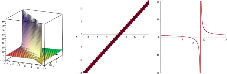
FIGURE 1

FIGURE 1. $ψ_{1}^{1} (x, y, z, t)$ : b₀ = 0, κ = δ = 0.6, α = β = 0.35, m = 0.06, ϖ = 0.5.

5 Results and Discussion

In this paper, SWL equation is examined using two exact methods, MAE method and extended $(\frac{G^{'}}{G^{2}})$ -expansion method. Both methods have provided trigonometric, hyperbolic and rational function solutions. However, the obtained solutions include a variety of distinct wave patterns. It can be observed that the MAE method has provided more solutions as compared to the extended $(\frac{G^{'}}{G^{2}})$ -expansion method.

The utilized mathematical techniques enable to construct possible variety of soliton solutions for arbitrary initial condition. The obtained solutions are useful to learn various kinds of wave structures which may be observed in any physical system governed by the GSWL equation. The physical structure of the waves expressed by the obtained solutions can be seen using graphical illustration. The 3D graphs of some of the retrieved solutions have been presented to show the shape of the corresponding wave. The graphs have been plotted using some suitable choice of parameters as described in the last section. The retrieved graphs depict a variety of physical behaviors depicting kink, periodic and bright-dark solitons which may appear in many phenomena involving shallow water waves.

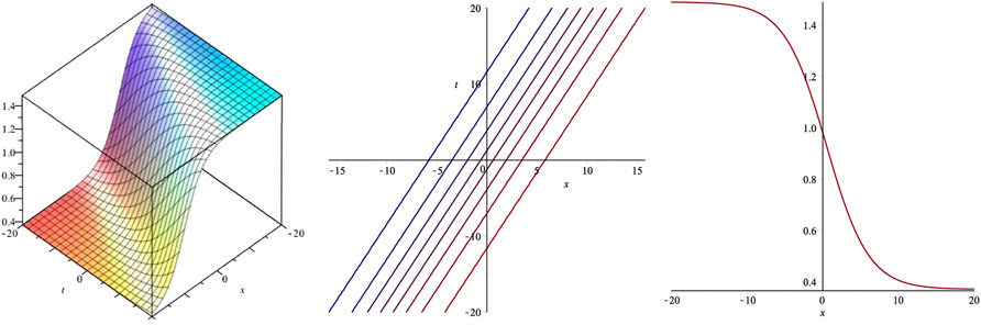
Figure 2 represents kink soliton solution as the graph of the function $ψ_{3}^{1}$ varies from one asymptotic state to another asymptotic state. Figure 5 represents the periodic wave solution as the wave pattern is repeated after equal intervals. The Figure 1, Figure 3 and Figure 6 represent the bright-dark singular soliton solutions as depicted by their line graphs at t = 1. Figure 4 is showing singular dark soliton solution as the intensity of wave is much lower at center of the wave than its neighboring points.

FIGURE 2

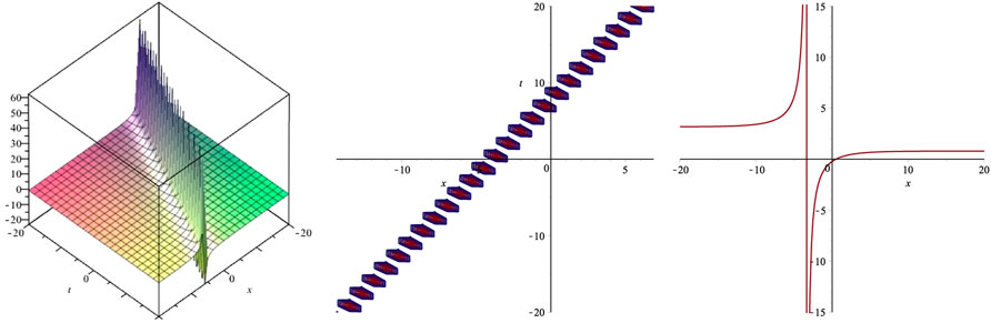
FIGURE 2. $ψ_{3}^{1} (x, y, z, t)$ : b₀ = 0, κ = δ = 0.6, α = β = 0.35, m = 0.06, ϖ = 0.5.

FIGURE 3

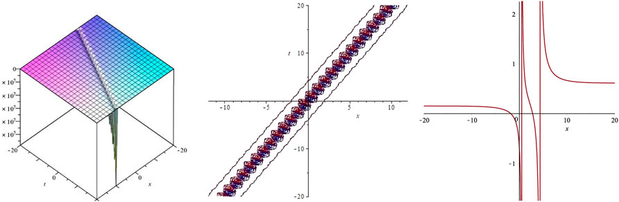
FIGURE 3. $ψ_{4}^{2} (x, y, z, t)$ : b₀ = 0, κ = δ = 0.6, α = β = 0.35, m = 0.06, ϖ = 0.5.

FIGURE 4

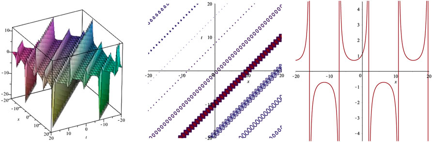
FIGURE 4. $ψ_{2}^{3} (x, y, z, t)$ : b₀ = 0, κ = δ = 0.6, α = β = 0.35, m = 0.06, ϖ = 0.5.

FIGURE 5

FIGURE 5. $ψ_{1}^{4} (x, y, z, t)$ : κ = 2, D = 6, rest of constants = 1.

FIGURE 6

FIGURE 6. $ψ_{2}^{4} (x, y, z, t)$ : κ = 2, D = 6, rest of constants = 1.

6 Conclusion

In this paper, the GSWL equation is discussed by MAE method and extended $(\frac{G^{'}}{G^{2}})$ -expansion method. Many soliton solutions containing rational, hyperbolic and trigonometric functions are obtained using proposed methods. The 3D surface graphs, 2D contour graphs and line graphs are plotted for retrieved solutions. The obtained graphs include kink soliton solutions, periodic solutions and bright-dark soliton solutions. It is worth mentioning that GSWL equation is discussed for the first time in this work by using proposed models. In future, GSWL equation can also be investigated using other methods, therefore much new work is yet to be done on this model.

Data Availability Statement

The original contributions presented in the study are included in the article/Supplementary Material, further inquiries can be directed to the corresponding authors.

Author Contributions

GA: Conceptualization, Methodology, Validation, Supervision, Visualization, Investigation. MS: Methodology, Validation, Investigation, Visualization, Writing- Reviewing and Editing. MK: Data Curation, Conceptualization, Methodology, Software, Writing- Original draft preparation.

Conflict of Interest

The authors declare that the research was conducted in the absence of any commercial or financial relationships that could be construed as a potential conflict of interest.

Publisher’s Note

All claims expressed in this article are solely those of the authors and do not necessarily represent those of their affiliated organizations, or those of the publisher, the editors and the reviewers. Any product that may be evaluated in this article, or claim that may be made by its manufacturer, is not guaranteed or endorsed by the publisher.

References

1. Kudryashov NA. Nonlinear Waves on Water and Theory of Solitons. J Eng Phys Thermophys (1999) 72(6):1224–35. doi:10.1007/bf02699470

CrossRef Full Text | Google Scholar

2. Kochanov MB, Kudryashov NA, Sinel'shchikov DI. Non-linear Waves on Shallow Water under an Ice Cover. Higher Order Expansions. J Appl Mathematics Mech (2013) 77(1):25–32. doi:10.1016/j.jappmathmech.2013.04.004

CrossRef Full Text | Google Scholar

3. Kudryashov NA, Soukharev MB, Demina MV. Elliptic Traveling Waves of the Olver Equation. Commun Nonlinear Sci Numer Simulation (2012) 17(11):4104–14. doi:10.1016/j.cnsns.2012.01.033

CrossRef Full Text | Google Scholar

4. Nisar KS, Ilhan OA, Abdulazeez ST, Manafian J, Mohammed SA, Osman MS. Novel Multiple Soliton Solutions for Some Nonlinear PDEs via Multiple Exp-Function Method. Results Phys (2021) 21:103769. doi:10.1016/j.rinp.2020.103769

CrossRef Full Text | Google Scholar

5. Seadawy AR, Lu D, Khater MAM. New Wave Solutions for the Fractional-Order Biological Population Model, Time Fractional Burgers, Drinfeld-Sokolov-Wilson and System of Shallow Water Wave Equations and Their Applications. Eur J Comput Mech (2017) 26(5-6):508–24. doi:10.1080/17797179.2017.1374233

CrossRef Full Text | Google Scholar

6. Yue C, Lu D, Khater MMA. Abundant Wave Accurate Analytical Solutions of the Fractional Nonlinear Hirota-Satsuma-Shallow Water Wave Equation. Fluids (2021) 6(7):235. doi:10.3390/fluids6070235

CrossRef Full Text | Google Scholar

7. Guo S, Zhou Y. The Extended -expansion Method and its Applications to the Whitham-broer-kaup-like Equations and Coupled Hirota-Satsuma KdV Equations (G′/G²) -expansion Method and its Applications to the Whitham-broer-kaup-like Equations and Coupled Hirota-Satsuma KdV Equations. Appl Mathematics Comput (2010) 215(9):3214–21. doi:10.1016/j.amc.2009.10.008

CrossRef Full Text | Google Scholar

8. Gao Y-T, Tian B. Generalized Tanh Method with Symbolic Computation and Generalized Shallow Water Wave Equation. Comput Mathematics Appl (1997) 33(4):115–8. doi:10.1016/s0898-1221(97)00011-4

CrossRef Full Text | Google Scholar

9. Zayed EME, Elshater MEM. Jacobi Elliptic Solutions, Soliton Solutions and Other Solutions to Four Higher-Order Nonlinear Schrodinger Equations Using Two Mathematical Methods. Optik (2017) 131:1044–62. doi:10.1016/j.ijleo.2016.11.120

CrossRef Full Text | Google Scholar

10. Zhou Q, Ekici M, Sonmezoglu A, Mirzazadeh M. Optical Solitons with Biswas-Milovic Equation by Extended G′/G-expansion Method. Optik (2016) 127(16):6277–90. doi:10.1016/j.ijleo.2016.04.119

CrossRef Full Text | Google Scholar

11. Kudryashov NA. Model of Propagation Pulses in an Optical Fiber with a New Law of Refractive Indices. Optik (2021) 248:168160. doi:10.1016/j.ijleo.2021.168160

CrossRef Full Text | Google Scholar

12. Kudryashov NA, Loguinova NB. Extended Simplest Equation Method for Nonlinear Differential Equations. Appl Mathematics Comput (2008) 205(1):396–402. doi:10.1016/j.amc.2008.08.019

CrossRef Full Text | Google Scholar

13. Miah MM, Ali HMS, Akbar A, Wazwaz MA. Some Applications of the (G′/G, 1/G)-expansion Method to Find New Exact Solutions of NLEEs. The Eur Phys J Plus (2017) 132(6):1–15. doi:10.1140/epjp/i2017-11571-0

CrossRef Full Text | Google Scholar

14. Dusunceli F. New Exact Solutions for Generalized (3+1) Shallow Water-like (SWL) Equation. Appl Mathematics Nonlinear Sci (2019) 4(2):365–70. doi:10.2478/amns.2019.2.00031

CrossRef Full Text | Google Scholar

15. Wazwaz A-M. Solitary Wave Solutions of the Generalized Shallow Water Wave (GSWW) Equation by Hirota's Method, Tanh-Coth Method and Exp-Function Method. Appl Mathematics Comput (2008) 202(1):275–86. doi:10.1016/j.amc.2008.02.013

CrossRef Full Text | Google Scholar

16. Sadaf M, Akram G. Effects of Fractional Order Derivative on the Solution of Time-Fractional Cahn-Hilliard Equation Arising in Digital Image Inpainting. Indian J Phys (2021) 95:891–9. doi:10.1007/s12648-020-01743-1

CrossRef Full Text | Google Scholar

17. Mahak N, Akram G. Exact Solitary Wave Solutions by Extended Rational Sine-Cosine and Extended Rational Sinh-Cosh Techniques. Phys Scr (2019) 94(11):115212. doi:10.1088/1402-4896/ab20f3

CrossRef Full Text | Google Scholar

18. Akram G, Sadaf M, Anum N. Solutions of Time-Fractional Kudryashov-Sinelshchikov Equation Arising in the Pressure Waves in the Liquid with Gas Bubbles. Opt Quan Electronics (2017) 49(11):1–16. doi:10.1007/s11082-017-1202-5

CrossRef Full Text | Google Scholar

19. Ekici M, Zhou Q, Sonmezoglu A, Moshokoa SP, Ullah MZ, Biswas A, et al. Solitons in Magneto-Optic Waveguides by Extended Trial Function Scheme. Superlattices and Microstructures (2017) 107:197–218. doi:10.1016/j.spmi.2017.04.021

CrossRef Full Text | Google Scholar

20. Vendhan CP. A Study of Berger Equations Applied to Non-linear Vibrations of Elastic Plates. Int J Mech Sci (1975) 17:461–8. doi:10.1016/0020-7403(75)90045-4

CrossRef Full Text | Google Scholar

21. Tariq H, Akram G. New Traveling Wave Exact and Approximate Solutions for the Nonlinear Cahn-Allen Equation: Evolution of a Nonconserved Quantity. Nonlinear Dyn (2017) 88(1):581–94. doi:10.1007/s11071-016-3262-7

CrossRef Full Text | Google Scholar

22. Akram G, Sadaf M, Khan MAU. Abundant Optical Solitons for Lakshmanan-Porsezian-Daniel Model by the Modified Auxiliary Equation Method. Optik (2022) 251:168163. doi:10.1016/j.ijleo.2021.168163

CrossRef Full Text | Google Scholar

23. Sadaf GAM, Khan MAU. Soliton Solutions of Lakshmanan-Porsezian-Daniel Model Using Modified Auxiliary Equation Method with Parabolic and Anti-cubic Law of Nonlinearities. Optik: Int J Light Electron Opt (2022) 252:168372. doi:10.1016/j.ijleo.2021.168372

CrossRef Full Text | Google Scholar

24. Osman MS, Lu D, Khater MMA, Attia RAM. Complex Wave Structures for Abundant Solutions Related to the Complex Ginzburg-Landau Model. Optik (2019) 192:162927. doi:10.1016/j.ijleo.2019.06.027

CrossRef Full Text | Google Scholar

25. Sirisubtawee S, Koonprasert S. Exact Traveling Wave Solutions of Certain Nonlinear Partial Differential Equations Using the (G′/G²)-expansion Method. Adv Math Phys (2018) 2018:7628651. doi:10.1155/2018/7628651

CrossRef Full Text | Google Scholar

Keywords: the generalized shallow water like equation, MAE method, extended (G′/G²)-expansion method, solitary wave solutions, exact solutions

Citation: Akram G, Sadaf M and Khan MAU (2022) Soliton Dynamics of the Generalized Shallow Water Like Equation in Nonlinear Phenomenon. Front. Phys. 10:822042. doi: 10.3389/fphy.2022.822042

Received: 25 November 2021; Accepted: 09 February 2022;
Published: 23 March 2022.

Edited by:

Lev Shchur, Landau Institute for Theoretical Physics, Russia

Reviewed by:

Sergey Moiseenko, Space Research Institute (RAS), Russia
Sergey Dmitrievich Glyzin, Yaroslavl State University, Russia

Copyright © 2022 Akram, Sadaf and Khan. This is an open-access article distributed under the terms of the Creative Commons Attribution License (CC BY). The use, distribution or reproduction in other forums is permitted, provided the original author(s) and the copyright owner(s) are credited and that the original publication in this journal is cited, in accordance with accepted academic practice. No use, distribution or reproduction is permitted which does not comply with these terms.

*Correspondence: Ghazala Akram, toghazala2003@yahoo.com; Maasoomah Sadaf, maasoomah.math@pu.edu.pk; M. Atta Ullah Khan, attaniazi271@gmail.com

ORIGINAL RESEARCH article

Soliton Dynamics of the Generalized Shallow Water Like Equation in Nonlinear Phenomenon

1 Introduction

2 Demarcation of Methods

2.1 The Algorithm of MAE Method

2.2 Extended (G′G2)-Expansion Method

3 The Application of Methods

3.1 The Application of MAE Method

3.2 The Application of Extended G′G2-Expansion Method

4 Graphical Explanation of Solutions

5 Results and Discussion

6 Conclusion

Data Availability Statement

Author Contributions

Conflict of Interest

Publisher’s Note

References

People also looked at

2.2 Extended $(\frac{G^{'}}{G^{2}})$ -Expansion Method

3.2 The Application of Extended $(\frac{G^{'}}{G^{2}})$ -Expansion Method