Finite difference schemes for MHD mixed convective Darcy–forchheimer flow of Non-Newtonian fluid over oscillatory sheet: A computational study

Nawaz, Yasir; Arif, Muhammad Shoaib; Abodayeh, Kamaleldin; Mansoor, Muavia

doi:10.3389/fphy.2023.1072296

ORIGINAL RESEARCH article

Front. Phys., 02 February 2023
Sec. Interdisciplinary Physics
Volume 11 - 2023 | https://doi.org/10.3389/fphy.2023.1072296

Finite difference schemes for MHD mixed convective Darcy–forchheimer flow of Non-Newtonian fluid over oscillatory sheet: A computational study

Yasir Nawaz¹

Muhammad Shoaib Arif^2,1* www.frontiersin.org

Kamaleldin Abodayeh²

Muavia Mansoor³

¹Department of Mathematics, Air University, Islamabad, Pakistan
²Department of Mathematics and Sciences, College of Humanities and Sciences, Prince Sultan University, Riyadh, Saudi Arabia
³Department of Mathematics, University of Wah, Wah Cant, Pakistan

This contribution proposes two third-order numerical schemes for solving time-dependent linear and non-linear partial differential equations (PDEs). For spatial discretization, a compact fourth-order scheme is deliberated. The stability of the proposed scheme is set for scalar partial differential equation, whereas its convergence is specified for a system of parabolic equations. The scheme is applied to linear scalar partial differential equation and non-linear systems of time-dependent partial differential equations. The non-linear system comprises a set of governing equations for the heat and mass transfer of magnetohydrodynamics (MHD) mixed convective Casson nanofluid flow across the oscillatory sheet with the Darcy–Forchheimer model, joule heating, viscous dissipation, and chemical reaction. It is noted that the concentration profile is escalated by mounting the thermophoresis parameter. Also, the proposed scheme converges faster than the existing Crank-Nicolson scheme. The findings that were provided in this study have the potential to serve as a helpful guide for investigations into fluid flow in closed-off industrial settings in the future.

1 Introduction

Electromagnetism and fluid mechanics share a modern scientific field called magnetohydrodynamics (MHD). The electromagnetic force, which has been widely exploited in many industries, such as semiconductor crystal growth, liquid metal blankets in nuclear fusion reactors, and steel-making processes, significantly hinders the flow of conducting materials.

Levitation of drops, dynamo modelling of planets, electromagnetic pumps, and other technologies. In light of these advancements, it is crucial to research significant MHD flows such as rotating, free-surface, and natural convection in rectangular ducts. Numerical analyses are being utilized to examine MHD flows that are more composite due to recent advancements in computational approaches. This Special Issue emphasized numerical and computational methods for deciphering and analyzing more complex MHD processes [1]. Miura [2] examined magneto hydrodynamic incompressible turbulence driven by gyro-viscous terms and Hall by numerical simulations of freely decaying, nearly isotropic, and homogeneous turbulent flow. He discovered that the Hall and gyro-viscous variables modify the energy transfer in the equations of motion to be predominantly forward transfer, while the magnetic energy transfer stays dominating.

The problem to be tackled in the present work is the Casson nanofluid flow across oscillatory surfaces with effects of joule heating, thermal radiations, and chemical reaction. Casson nan fluid is preferable to Newtonian-based nan fluid flow as cooling and friction-reducing agents [3]. Casson introduced the Casson fluid model for the movement of viscoelastic liquids in 1959. Stress at which no flow occurs should be provided by the Casson fluid, a shear-thinning fluid, which should have infinite viscosity at zero rates of shear and zero viscosity at infinite rates of shear. Casson fluid includes honey, jelly, sauce, soup, and other things [4]. Ali et al.'s [5] investigation of the Casson fluid flow on a tilted sheet included the Soret-Dufour effects. Manideep et al. [6] studied the fluid Casson flow on vertically inclined sheets. Shamshuddin et al. [7] conducted a statistical analysis of a chemical reaction’s impact on the Casson fluid flow on a sloped plate [8]; Vijayaragavan and Kavitha estimated the Casson fluid flow over a tilted plate. Taking into account the current hall, Prasad et al. [9] studied Casson fluid flow on an inclined sheet. The inclined Casson fluid flow on a permeable sheet was studied by Jain and Parmar [10]. The angle effect was considered in Sailaja et al. [11].'s study of the Casson fluid flow on a vertical sheet. Casson fluid flow was investigated by Rawi et al. [12] on a slanted sheet to take nanoparticles into account. Rauju et al. [13] discussed Casson fluid flow on a vertically inclined sheet in their study. The Casson fluid model performs better with blood.

According to the literature, chemical reactions can be divided into boundary or single-phase volumetric reactions, while homo-heterogeneous reactions depend on both. In cases like the creation of smog, first-order homogeneous chemical processes are discussed. The hydrometallurgical and chemical industries are particularly affected by the results of chemical processes involving mass transfer. Since they are inversely correlated with species concentration, reaction rates are frequently thought of as first order. Outside chemicals trigger chemical reactions in the water or the atmosphere. Heat is frequently produced between two species when chemical processes occur, the existence of reactions, and viscous dissipation. The unsteady MHD flow over an extended surface with varying viscosity was studied by Kishan and Hunegnaw [14] while it was embedded in an incredibly porous material. By involving energy and reaction over a parabolic surface using a finite element approach, Y. M. Chu et al. [15] examine the enhancement of thermal energy and solute particles using hybrid nanoparticles. References [16, 17] provide additional details.

A phenomenon of warmth transmission by radiation could be thermal radiation. Due to the high thermal effects involved in the production of electrical engineering and industrial significance can be seen in the cooling of metallic items, paper plates, petroleum pumps, and chips and their effects on MHD [3, 18–20] flows. Applications of radiation effects in physics and engineering processes are considerable. It significantly affects space technology, which studies the thermal effects of various fluxes, and processes that warm solids or liquids. The impacts of thermal radiation might be extremely important in controlling heat transfer in the polymer manufacturing industry, where the value of the materials is focused on heat-maintaining qualities. A bi-viscosity fluid confined in a highly trapezoidal cavity is analyzed by Nasir et al. [21] under the influence of thermal and magnetic forces. According to Kumar et al., the non-linear thermal radiation influence needs to be studied to analyze MHD shear-thickening fluid motion through stretchy geometry, according to Kumar et al. [22]. The effects of thermal radiations on heat transfer for Casson fluid flow in porous media across a non-linearly growing surface are examined by Pramanik [23]. Refs [24–27] provide more details about recent investigations.

Joule heating is when current energy is modified to heat because of flow in resistance. It's a good range of applications, like in industries and technology. The Joule heating effect occurs when an electric current flows through a conductor and causes heat to be generated. The Joule heating effect is used in many industrial processes and devices. In addition to food processing and scanning microscopes, infrared-thermal images, electrical radiative heaters, light bulbs, laboratory water baths, electric tabletop hotplates, clothes irons, hand tools, fan heaters, hair dryers, and cartridge heaters are among the several uses for heating effects of a joule. The researchers and engineers reviewed the Joule heating effect in their respective fields of study in light of the abovementioned applications. The fluid temperature rose for the joule heating parameter for a hyperbolic tangent nanofluid in porous media in a study by Alaidrous et al. [28]. In addition to taking into account the features of the Cattaneo-Christove heat flux theory, Hafeez et al. [29] explored the Oldroyd-B nan non-Newtonian fluid flow. According to this work, the concentration of Oldroyd-B nanofluid increases for thermophoresis. An investigation by Khan et al. [30] determined that the force field parameter increases the nan fluid velocity profile in Casson nanofluid flow through a rotating cylinder that is hydromagnetic in three dimensions, with consequences of entropy and Joule heating. Kumar et al. [31] used the shot method and the RK4 scheme to examine the effects of the Joule heating effect on the flow of Williamson nano fluid toward the stretching sheet. The entropy of the system rises as the Brinkman parameter is advanced. As a cylinder shrinks, a highly hybrid nanofluid flows through it. Khashi’ie et al. [32] investigated the effects of Joule heating and warmth transmission. Uddin et al. [33] identified the multiple features of the Joule heating effect on the mixed convection MHD flow. Our investigation leads us to the conclusion that the fabric magnetic parameter enhanced the skin friction coefficient. Kazemi et al. [34] proposed an analytical solution for the fourth-grade nan fluid flow along the duct walls in viscous dissipation and Joule heating forces. According to their research, heat transport via duct walls may reduce by up to 40% when the Hartman number is raised. Rasheed et al. [35] investigated the Jeffery nano liquid MHD boundary flow over an extended cylinder with heat generation and absorption consequences. The Darcy–Forchheimer flow of Williamson fluid over a Riga plate under the effects of suction/injection has been explained in [36]. The heat and mass transfer were also considered with the effect of heat consumption/generation. For solving the ODEs in the presented phenomenon, both numerical and analytical studies were carried out. The numerical solution was based on applying Matlab solver bvp4c, and the analytical study was based on the analytical method named homotopy analysis method. From the obtained results, it was seen that fluid temperature was raised by increasing radiation parameters. A Buongiorno nanofluid model has been considered in [37] for investigating electro-magneto hydrodynamic flow over a Riga plate. A nanofluid model was considered with Cattaneo-Christov’s heat flux and generalized Fick’s law. A study of MHD micropolar ferrofluid flow over a stretching surface has been given in [38]. Using the similarity transformations, the governing equations of flow were reduced into a set of ODEs and solved by Matlab solver bvp4c. It was observed that stream function and velocity declined by enhancing magnetic parameters. Matrix nanocomposites are materials with various applications because of their thermophysical properties.

An all-encompassing numerical study of the many physical features of steady MHD Von Kármán’s flows of chemically reacting nanofluids that can occur over a rotating disk in the presence of a radially applied magnetic field has been performed in [39]. This is done under the assumption that the disk surface is impermeable and heated convectively, in which case the vertical nanoparticles’ mass flux has practically vanished. Examining how the generalized heat transport affects the free convection flow of a viscous nanofluid in a cylinder is what [40] is all about. The heat transfer equation is generalized using the generalized Atangana–Baleanu time-fractional differential operator.

The study for the dispersion of matric nanocomposite material on magnetized nanofluid flow over the coaxial disks was given in [41]. The prominence of the permeability function was also examined numerically. The calculated results showed that the increasing nanolayer thickness had escalated thermal phenomena and effective nanolayer thermal conductivity. It was also noticed that the Nusselt number was enhanced by incrementing hybrid nanoparticles volume fraction. Ferrofluid is made up of tiny magnetic particles and uses in inertial and viscous damping, dynamic sealing and magnetic drug targeting. The study of this fluid has been given in [38], and the stretching sheet caused the flow. For solving ODEs obtained by applying transformations to the governing equations of the fluid flow, Matlab solver bvp4c has been employed. It was observed that stream function and velocity declined by enhancing magnetic parameters. In [42], an infinite medium was used to investigate a thermoelastic diffusion model of fractional order. An inclined temperature field was transmitted through the spherical cavity. The eigenvalue technique solved the differential equation in the form of vector-matric equation in the Laplace transform domain. An analytical solution for the displacement, temperature, and concentration was found in the Laplace domain. A finite element method is one of the numerical methods that can be considered to solve ordinary and partial differential equations. This method has been considered in [43] to study the dual-phase-lag model on thermoelastic interaction subjected to a ramp type of heating. The method was proposed to solve the problem and found the solutions for displacement, temperature and stress. A comparison for some results was also given with three theories. Some more recent work on MHD flow can be found [44–46].

The motivation of this contribution is based on the modifications of analytical methods which have been done earlier, and this effort is not to modify some numerical method. The modification of the numerical method is the main objective of this work and its application to some applied problems in science or engineering. The numerical technique is applied to Casson fluid flow over the oscillatory plate. The non-Newtonian MHD fluid has applications in heat storage beds, textile industries, irrigation problems and polymer composite industries.

In literature, numerous numerical methods exist for solving different types of problems in science and engineering. Some methods discretize only the time variable in the time-dependent PDEs. The time discretization methods can be classified into two types. One of these types of methods is an explicit class of methods, and the second is an implicit class of methods. Explicit methods mostly have smaller stability regions than those provided by some implicit methods. Explicit methods are easy to employ for any non-linear problem, but implicit types of methods require linearized differential equations. Also, the systems of equations obtained by employing implicit methods are required to solve by any software solver solving equations, or these systems require any other iterative method. In this contribution, the Gauss-Seidel iterative method is employed for solving equations after applying the proposed numerical scheme. The proposed numerical schemes are constructed on three-time levels. The first stage is constructed on two-time levels, whereas the second stage uses the information of three-time levels to find the solution at some particular time level. So, a second stage requires any other method based on two levels to find the solution at the first time level. The scheme is applied to two problems: one is a linear problem, and the second is a system of non-linear PDEs. The system of non-linear parabolic equations is obtained from the phenomenon of nanofluid flow over the oscillatory sheet. Effects of heat and mass transfer, thermal radiation, viscous dissipation, and joule heating are also considered. The system is first reduced into dimensionless PDEs and later solved by the proposed scheme with fourth-order compact discretization in space. Analytical and numerical methods can be used to solve considered flow problems. The numerical methods may comprise the finite element method and high-order finite difference approaches that can be used to discretize time and spatial terms in the given PDE. Since this contribution aims to propose a numerical method, its application to the flow problem is also given. Because of this study, more computational schemes can be constructed that will have more advantages than these schemes.

2 Numerical scheme

The proposed numerical scheme is a two-stage scheme consisting of explicit and implicit stages. The explicit stage is the forward Euler method, whereas the implicit stage comprises some unknown parameters. The first stage finds the problem’s solution at some unknown time level. The second stage of the scheme uses the information of the solution computed from the first stage of the scheme and finds a solution at $(n + 1) t h$ time level. For proposing a scheme, consider the time-dependent partial differential equation in the form of

\frac{\partial u}{\partial t} = f (u, \frac{\partial^{2} u}{\partial x^{2}}), (1)

subject to the boundary conditions

u (t, - L) = α_{1}, u (t, L) = α_{2}, (2)

where $α_{1}$ and $α_{2}$ are constants which have the same dimensions as the dependent variable $u$ , and the initial condition can be given as

u (0, x) = g (x), (3)

where $g (x)$ is the function that only depends on $x$ .

The first stage of the scheme is given as,

{\bar{u}}_{i}^{n + 1} = u_{i}^{n} + Δ t {\frac{\partial u}{\partial t}|}_{i}^{n}, (4)

This stage 4) requires only the information of the dependent variable computed at the previous time level. The next stage consists of a difference equation that contains some unknown parameters. The second stage of the scheme with unknown constant parameters $a_{1}, a_{2}, a_{3} & a_{4}$ can be expressed as:

u_{i}^{n + 1} = u_{i}^{n} + Δ t \{a_{1} {\frac{\partial u}{\partial t}|}_{i}^{n + 1} + a_{2} {\frac{\partial u}{\partial t}|}_{i}^{n} + a_{3} {\frac{\partial \bar{u}}{\partial t}|}_{i}^{n}\} + a_{4} {(Δ t)}^{2} {\frac{\partial^{2} u}{\partial t^{2}}|}_{i}^{n}, (5)

The unknown parameters $a_{1}, a_{2}, a_{3}$ and $a_{4}$ can be found by using Taylor series expansions for $u_{i}^{n + 1}$ and ${\frac{\partial u}{\partial t}|}_{i}^{n}$ , as follows

\begin{array}{c} u_{i}^{n + 1} = u_{i}^{n} + Δ t {\frac{\partial u}{\partial t}|}_{i}^{n} + \frac{{(Δ t)}^{2}}{2} {\frac{\partial^{2} u}{\partial t^{2}}|}_{i}^{n} + \frac{{(Δ t)}^{3}}{6} {\frac{\partial^{3} u}{\partial t^{3}}|}_{i}^{n} + O ({(Δ t)}^{4}), \\ {\frac{\partial u}{\partial t}|}_{i}^{n + 1} = {\frac{\partial u}{\partial t}|}_{i}^{n} + Δ t {\frac{\partial^{2} u}{\partial t^{2}}|}_{i}^{n} + \frac{{(Δ t)}^{2}}{2} {\frac{\partial^{3} u}{\partial t^{3}}|}_{i}^{n} + O ({(Δ t)}^{3}) . \end{array}\} (6)

Substituting 4) and 6) into Eq. 5, it is obtained

\begin{align} u_{i}^{n} + Δ t {\frac{\partial u}{\partial t}|}_{i}^{n} + \frac{{(Δ t)}^{2}}{2} {\frac{\partial^{2} u}{\partial t^{2}}|}_{i}^{n} + \frac{{(Δ t)}^{3}}{6} {\frac{\partial^{3} u}{\partial t^{3}}|}_{i}^{n} & = u_{i}^{n} + Δ t \{{a_{1} \frac{\partial u}{\partial t}|}_{i}^{n} + a_{1} Δ t {\frac{\partial^{2} u}{\partial t^{2}}|}_{i}^{n} + a_{1} \frac{{(Δ t)}^{2}}{2} {\frac{\partial^{3} u}{\partial t^{3}}|}_{i}^{n} + a_{2} {\frac{\partial u}{\partial t}|}_{i}^{n} + a_{3} {\frac{\partial u}{\partial t}|}_{i}^{n} + a_{3} Δ t {\frac{\partial^{2} u}{\partial t^{2}}|}_{i}^{n}\} \\ + {(Δ t)}^{2} a_{4} {\frac{\partial^{2} u}{\partial t^{2}}|}_{i}^{n} . \end{align} (7)

Comparing coefficients of $a_{1}, a_{2}, a_{3}$ and $a_{4}$ from Eq. 7, it is obtained

1 = a_{1} + a_{2} + a_{3}, (8)

\frac{1}{2} = a_{1} + a_{3} + a_{4}, (9)

\frac{1}{6} = \frac{a_{1}}{2} . (10)

By solving Eqs. 8–10, the values for $a_{1}, a_{2}, a_{3}$ and $a_{4}$ can be obtained as:

a_{1} = \frac{1}{3}, a_{2} = \frac{1}{2} + a_{4}, a_{3} = \frac{1}{6} - a_{4} . (11)

Therefore, the second stage of the proposed scheme for time discretization of Eq. 1 can be expressed as:

u_{i}^{n + 1} = u_{i}^{n} + Δ t \{\frac{1}{3} {\frac{\partial u}{\partial t}|}_{i}^{n + 1} + (\frac{1}{2} + a_{4}) {\frac{\partial u}{\partial t}|}_{i}^{n} + (\frac{1}{6} - a_{4}) {\frac{\partial \bar{u}}{\partial t}|}_{i}^{n}\} + a_{4} {(Δ t)}^{2} {\frac{\partial^{2} u}{\partial t^{2}}|}_{i}^{n} . (12)

In Eq. 12, $a_{4}$ is a free parameter, and the suitable value of this parameter can be chosen so that the stable solution can be obtained.

Since the suggested scheme is only a time discretization scheme that can be used to discretize time derivative terms in considered time-dependent PDEs, it is to be noted that a semi-discrete scheme (12) can only be used to discretize time derivative terms. Space discretization can be performed by employing any scheme that discretizes spatial term(s) in given partial differential equations. For this contribution, a compact fourth-order scheme is adopted that can be used to discretize space derivative term(s). The adopted compact scheme requires finding the additional partial derivative of the given differential equation.

Applying a compact scheme to Eq. 1 using $f = \frac{\partial^{2} u}{\partial x^{2}},$ it gives

{\frac{\partial u}{\partial t}|}_{i} = {δ_{x}^{2} u|}_{i} - \frac{{(Δ x)}^{2}}{12} {\frac{\partial^{4} u}{\partial x^{4}}|}_{i} . (13)

where ${δ_{x}^{2} u|}_{i} = \frac{u_{i + 1} - 2 u_{i} + u_{i - 1}}{{(Δ x)}^{2}}$ and $Δ x$ is the spatial step.

Since Eq. 13 requires finding a fourth-order spatial derivative term, which will be found from Eq. 1 using $f = \frac{\partial^{2} u}{\partial x^{2}}$ as

\frac{\partial^{4} u}{\partial x^{4}} = \frac{\partial}{\partial t} {δ_{x}^{2} u|}_{i} . (14)

Substituting Eq. 14 into Eq. 13 gives

{\frac{\partial u}{\partial t}|}_{i} = {δ_{x}^{2} u|}_{i} - \frac{{(Δ x)}^{2}}{12} \frac{\partial}{\partial t} {δ_{x}^{2} u|}_{i} . (15)

Equation 15 can be re-written as

\frac{\partial}{\partial t} ({u|}_{i} + \frac{{(Δ x)}^{2}}{12} \frac{\partial}{\partial t} {δ_{x}^{2} u|}_{i}) = {δ_{x}^{2} u|}_{i} . (16)

Employing the first stage of the proposed scheme in Eq. 16 yields

{\bar{u}}_{i}^{n + 1} + \frac{{(Δ x)}^{2}}{12} δ_{x}^{2} {\bar{u}}_{i}^{n + 1} = u_{i}^{n} + \frac{{(Δ x)}^{2}}{12} δ_{x}^{2} u_{i}^{n} + Δ t δ_{x}^{2} u_{i}^{n} . (17)

Applying the second stage of the proposed scheme to Eq. 16, it follows

u_{i}^{n + 1} + \frac{{(Δ x)}^{2}}{12} δ_{x}^{2} u_{i}^{n + 1} = u_{i}^{n} + \frac{{(Δ x)}^{2}}{12} δ_{x}^{2} u_{i}^{n} + Δ t \{\begin{array}{c} \frac{1}{3} δ_{x}^{2} u_{i}^{n + 1} + (\frac{1}{2} + a_{4}) δ_{x}^{2} u_{i}^{n} + \\ (\frac{1}{6} - a_{4}) δ_{x}^{2} {\bar{u}}_{i}^{n + 1} + Δ t a_{4} {\frac{\partial^{2} u}{\partial t^{2}}|}_{i}^{n} \end{array}\} . (18)

Since Eq. 18 contains second order time derivative term, that can be found by finding the second partial derivative of Eq. 1 using $f = \frac{\partial^{2} u}{\partial x^{2}}$ . Alternatively, this second-order partial time derivative in Eq. 18 can be numerically approximated by the second-order central difference formula as:

{\frac{\partial^{2} u}{\partial t^{2}}|}_{i}^{n} = \frac{u_{i}^{n + 1} - 2 u_{i}^{n} + u_{i}^{n - 1}}{{(Δ t)}^{2}} (19)

Substituting Eq. 19 into Eq. 18, it follows

u_{i}^{n + 1} + \frac{{(Δ x)}^{2}}{12} δ_{x}^{2} u_{i}^{n + 1} = u_{i}^{n} + \frac{{(Δ x)}^{2}}{12} δ_{x}^{2} u_{i}^{n} + Δ t {\frac{1}{3} δ_{x}^{2} u_{i}^{n + 1} + (\frac{1}{2} + a_{4}) δ_{x}^{2} u_{i}^{n} + (\frac{1}{6} - a_{4}) δ_{x}^{2} {\bar{u}}_{i}^{n + 1}} + a_{4} (u_{i}^{n + 1} - 2 u_{i}^{n} + u_{i}^{n - 1}) (20)

3 Stability analysis

The stability analysis for linear parabolic PDEs will be presented. This stability analysis gives the condition on the ratio of temporal step size and squared spatial step size, called diffusion number. So, a scheme with a large stability region might be preferred more than a smaller one. The scheme with a large stability region gives a large choice of step sizes and larger intervals for numerical values of involved parameters. So, the time consumed by the code for those schemes with large stability regions will be smaller than others. To start the stability analysis of the proposed scheme for classical or standard parabolic Eq. 1 using $f = \frac{\partial^{2} u}{\partial x^{2}}$ . Following transformations will be applied:

\begin{array}{c} {\bar{u}}_{i}^{n + 1} = E^{n + 1} e^{i I ψ}, u_{i \pm 1}^{n} = E^{n} e^{(i \pm 1) I ψ} \\ u_{i}^{n + 1} = E^{n + 1} e^{i I ψ}, u_{i \pm 1}^{n + 1} = E^{n + 1} e^{(i \pm 1) I ψ} \\ u_{i}^{n - 1} = E^{n - 1} e^{i I ψ} \end{array}\} (21)

Substituting some of the transformations from Eq. 21 into Eq. 17 yields

{\bar{E}}^{n + 1} e^{i I ψ} + \frac{{(Δ x)}^{2}}{12} (\frac{e^{(i + 1) I ψ} - 2 e^{i I ψ} + e^{(i - 1) I ψ}}{{(Δ x)}^{2}}) E^{n + 1} = E^{n} e^{i I ψ} + \frac{{(Δ x)}^{2}}{12} (\frac{e^{(i + 1) I ψ} - 2 e^{i I ψ} + e^{(i - 1) I ψ}}{{(Δ x)}^{2}}) E^{n} + \frac{Δ t}{{(Δ x)}^{2}} (e^{(i + 1) I ψ} - 2 e^{i I ψ} + e^{(i + 1) I ψ}) E^{n} (22)

where $I = \sqrt{- 1}$ .

Dividing both sides of Eq. 22 by $e^{i I ψ}$ , it yields

{\bar{E}}^{n + 1} (1 + \frac{1}{6} (\cos ψ - 1)) = E^{n} + \frac{1}{6} (\cos ψ - 1) E^{n} + 2 d (\cos ψ - 1) E^{n} . (23)

Re-write Eq. 23 as

{\bar{E}}^{n + 1} = \frac{[\frac{5}{6} + \frac{1}{6} \cos ψ + 2 d (\cos ψ - 1)] E^{n}}{\frac{5}{6} + \frac{1}{6} \cos ψ} (24)

Substituting transformation from (21) into Eq. 20, it follows:

\begin{matrix} E^{n + 1} e^{i I ψ} + \frac{1}{12} (e^{(i + 1) I ψ} - 2 e^{i I ψ} + e^{(i - 1) I ψ}) E^{n + 1} \\ = E^{n} e^{i I ψ} + \frac{1}{12} (e^{(i + 1) I ψ} - 2 e^{i I ψ} + e^{(i - 1) I ψ}) E^{n} \\ + d \frac{1}{3} (e^{(i + 1) I ψ} - 2 e^{i I ψ} + e^{(i - 1) I ψ}) E^{n + 1} + (\frac{1}{2} + a_{4}) (e^{(i + 1) I ψ} - 2 e^{i I ψ} + e^{(i - 1) I ψ}) E^{n} \\ + (\frac{1}{6} - a_{4}) (e^{(i + 1) I ψ} - 2 e^{i I ψ} + e^{(i - 1) I ψ}) {\bar{E}}^{n + 1} \\ + a_{4} (E^{n + 1} - 2 E^{n} + E^{n - 1}) \end{matrix} (25)

Dividing both sides of Eq. 25 by $e^{i I ψ}$ and substituting Eq. 24 into the resulting equation, it is obtained

\begin{matrix} E^{n + 1} [1 + \frac{1}{6} (\cos ψ - 1) - \frac{2}{3} d (\cos ψ - 1) a_{4}] \\ = [1 + \frac{1}{6} (\cos ψ - 1) + 2 d (\frac{1}{2} + a_{4}) (\cos ψ - 1) + (\frac{1}{6} - a_{4}) (\cos ψ - 1) [\frac{\frac{5}{6} + \frac{1}{6} \cos ψ + 2 d (\cos ψ - 1)}{\frac{5}{6} + \frac{1}{6} \cos ψ}] - 2 a_{4}] E^{n} + a_{4} E^{n - 1} . \end{matrix} (26)

Equation 26 can be re-written as

E^{n + 1} = \bar{a} E^{n} + \bar{b} E^{n - 1} . (27)

where $\bar{a} = \frac{\frac{5}{6} + \frac{1}{6} \cos ψ + 2 d (\frac{1}{2} + a_{4}) (\cos ψ - 1) + (\frac{1}{6} - a_{4}) (\cos ψ - 1) \{\frac{\frac{5}{6} + \frac{\cos ψ}{6} + 2 d (\cos ψ - 1)}{\frac{5}{6} + \frac{\cos ψ}{6}}\} - 2 a_{4}}{\frac{5}{6} + \frac{\cos ψ}{6} - \frac{2}{3} d (\cos ψ - 1) - a_{4}}$ , $\bar{b} = \frac{a_{4}}{\frac{5}{6} + \frac{\cos ψ}{6} - \frac{2}{3} d (\cos ψ - 1) - a_{4}}$

Since the proposed scheme is constructed on three-time levels, finding an amplification matrix requires one more equation. Also, note that the stability condition can be found without constructing an additional equation. But for this stability analysis, an additional condition is required. The additional equation is constructed as:

E^{n} = E^{n} + 0 E^{n - 1} . (28)

The vector matrix equation can be obtained from Eqs. 27, 28 as

[\begin{array}{c} E^{n + 1} \\ E^{n} \end{array}] = [\begin{array}{c} \bar{a} & \bar{b} \\ 1 & 0 \end{array}] [\begin{array}{c} E^{n} \\ E^{n - 1} \end{array}] (29)

The stability condition will be imposed on the Eigenvalues of the coefficients matrix of Eq. 29, which can be expressed as:

λ_{1} = \frac{\bar{a} - \sqrt{{\bar{a}}^{2} + 4 \bar{b}}}{2} and λ_{2} = \frac{\bar{a} + \sqrt{{\bar{a}}^{2} + 4 \bar{b}}}{2} . (30)

The stability conditions can be written as

|λ_{1}| \leq 1 and |λ_{2}| \leq 1 . (31)

So, if a scheme satisfies condition (31), it will be stable. A more detailed explanation of the stability condition can be obtained from a graphical view of condition (31). Those values of diffusion number $″ d ″$ that satisfy condition (31) can be chosen for converged solutions.

4 Problem formulation

This contribution also consisted of the mathematical model of boundary layer flow over the oscillatory sheet. The mathematical model will be comprised of a system of parabolic PDEs. One must first construct a matrix equation and discretize it using the compact scheme in the spatial direction and the proposed scheme in the temporal direction before determining the convergence condition for a system of PDEs. For this reason, consider a matrix vector equation of the form

\frac{\partial v}{\partial t} = A \frac{\partial^{2} v}{\partial y^{2}} + B \frac{\partial v}{\partial y} + C v (32)

where $A, B,$ and $C$ are $3 \times 3$ matrices, and $v$ is a vector having three entries. By employing a fourth-order compact discretization to Eq. 31, the following semi-discretize scheme can be obtained:

\frac{\partial}{\partial t} [{v|}_{i} + \frac{{(Δ y)}^{2}}{12} (δ_{y}^{2} {v|}_{i} + B A^{- 1} δ_{y} {v|}_{i})] = (A + C \frac{{(Δ y)}^{2}}{12} + \frac{{(Δ y)}^{2}}{12} B A^{- 1} B) δ_{y}^{2} {v|}_{i} + (B + \frac{{(Δ y)}^{2}}{12} B A^{- 1} C) δ_{y} {v|}_{i} + C {v|}_{i} . (33)

Applying the first stage of the proposed scheme to Eq. 33, is obtained

\begin{matrix} {\bar{v}}_{i}^{n + 1} + \frac{{(Δ y)}^{2}}{12} (δ_{y}^{2} {\bar{v}}_{i}^{n + 1} + B A^{- 1} δ_{y} {\bar{v}}_{i}^{n + 1}) - v_{i}^{n} - \frac{{(Δ y)}^{2}}{12} (δ_{y}^{2} v_{i}^{n} + B A^{- 1} δ_{y} v_{i}^{n}) \\ = Δ t (A + C \frac{{(Δ y)}^{2}}{12} + \frac{{(Δ y)}^{2}}{12} B A^{- 1} B) δ_{y}^{2} v_{i}^{n} \\ + Δ t (B + \frac{{(Δ y)}^{2}}{12} B A^{- 1} C) δ_{y} v_{i}^{n} + Δ t C v_{i}^{n} \end{matrix} (34)

Now applying the second stage of the proposed scheme on Eq. 33, yields

\begin{matrix} v_{i}^{n + 1} + \frac{{(Δ y)}^{2}}{12} (δ_{y}^{2} v_{i}^{n + 1} + B A^{- 1} δ_{y} v_{i}^{n + 1}) - v_{i}^{n} - \frac{{(Δ y)}^{2}}{12} (δ_{y}^{2} v_{i}^{n} + B A^{- 1} δ_{y} v_{i}^{n}) \\ = Δ t \{a_{1} (A_{1} δ_{y}^{2} v_{i}^{n + 1} + B_{1} δ_{y} v_{i}^{n + 1} + C v_{i}^{n + 1}) + b_{1} (A_{1} δ_{y}^{2} v_{i}^{n} + B_{1} δ_{y} v_{i}^{n} + C v_{i}^{n}) + c_{1} (A_{1} δ_{y}^{2} {\bar{v}}_{i}^{n + 1} + B_{1} δ_{y} {\bar{v}}_{i}^{n + 1} + C {\bar{v}}_{i}^{n + 1})\} \\ + e_{1} (v_{i}^{n + 1} - 2 v_{i}^{n} + v_{i}^{n - 1}) \end{matrix} (35)

Theorem 4.1:. The scheme given in the form of Eqs. (34)-(35) converges.

Proof:. Let the first stage of the exact scheme be expressed as:

{\bar{V}}_{i}^{n + 1} + \frac{{(Δ y)}^{2}}{12} (δ_{y}^{2} {\bar{V}}_{i}^{n + 1} + B A^{- 1} δ_{y} {\bar{V}}_{i}^{n + 1}) - V_{i}^{n} - \frac{{(Δ y)}^{2}}{12} (δ_{y}^{2} V_{i}^{n} + B A^{- 1} V_{i}^{n}) = Δ t A_{1} δ_{y}^{2} V_{i}^{n} + Δ t B_{1} δ_{y} V_{i}^{n} + Δ t C V_{i}^{n} . (36)

Let the error be ${\bar{v}}_{i}^{n + 1} - {\bar{V}}_{i}^{n + 1} = {\bar{e}}_{i}^{n + 1}$ and subtracting Eq. 36 from Eq. 34, it is obtained

{\bar{e}}_{i}^{n + 1} + \frac{{(Δ)}^{2}}{12} (δ_{y}^{2} {\bar{e}}_{i}^{n + 1} + B A^{- 1} δ_{y} {\bar{e}}_{i}^{n + 1}) - e_{i}^{n} - \frac{{(Δ y)}^{2}}{12} (δ_{y} e_{i}^{n} + B A^{- 1} δ_{y} e_{i}^{n}) = Δ t A_{1} δ_{y}^{2} e_{i}^{n} + Δ t B_{1} δ_{y} e_{i}^{n} + Δ t C e_{i}^{n} . (37)

Re-write Eq. 37 as

\frac{5}{6} {\bar{e}}^{n + 1} + \frac{{(Δ)}^{2}}{12} (\frac{{\bar{e}}_{i + 1}^{n + 1} + {\bar{e}}_{i - 1}^{n + 1}}{{(Δ y)}^{2}} + B A^{- 1} δ_{y} {\bar{e}}_{i}^{n + 1}) - e_{i}^{n} - \frac{{(Δ y)}^{2}}{12} (δ_{y}^{2} e_{i}^{n} + B A^{- 1} δ_{y} e_{i}^{n}) = Δ t A_{1} δ_{y}^{2} e_{i}^{n} + Δ t B_{1} δ_{y} e_{i}^{n} + Δ t C e_{i}^{n} (38)

Applying the norm on both sides of Eq. 38 and re-write the resulting equation in the form of

{\bar{e}}^{n + 1} \leq γ_{1} e^{n}, (39)

where $γ_{1} = \frac{1 + \frac{{(Δ y)}^{2}}{12} (\frac{4}{{(Δ y)}^{2}} + \frac{‖B A^{- 1}‖}{Δ y}) + 4 d ‖A_{1}‖ + c ‖B_{1}‖ + Δ t ‖C‖}{\frac{2}{3} - \frac{Δ y}{12} ‖B A^{- 1}‖}$ .Now consider the second stage of the exact scheme for Eq. 32 can be expressed as:

\begin{matrix} V_{i}^{n + 1} + \frac{{(Δ y)}^{2}}{12} (δ_{y}^{2} V_{i}^{n + 1} + B A^{- 1} δ_{y} V_{i}^{n + 1}) - V_{i}^{n} - \frac{{(Δ y)}^{2}}{12} (δ_{y}^{2} V_{i}^{n} + B A^{- 1} δ_{y} V_{i}^{n}) \\ = Δ t \{a_{1} (A_{1} δ_{y}^{2} V_{i}^{n + 1} + B_{1} δ_{y} V_{i}^{n + 1} + C V_{i}^{n + 1}) + b_{1} (A_{1} δ_{y}^{2} V_{i}^{n} + B_{1} δ_{y} V_{i}^{n} + C V_{i}^{n}) + c_{1} (A_{1} δ_{y}^{2} {\bar{V}}_{i}^{n + 1} + B_{1} δ_{y} {\bar{V}}_{i}^{n + 1} + C {\bar{V}}_{i}^{n + 1})\} \\ + e_{1} (V_{i}^{n + 1} - 2 V_{i}^{n} + V_{i}^{n - 1}) . \end{matrix} (40)

Subtracting Eq. 40 from Eq. 35 gives

\begin{matrix} e_{i}^{n + 1} + \frac{{(Δ)}^{2}}{12} (δ_{y}^{2} e_{i}^{n + 1} + B A^{- 1} δ_{y} e_{i}^{n + 1}) - e_{i}^{n} - \frac{{(Δ y)}^{2}}{12} (δ_{y}^{2} e_{i}^{n} + B A^{- 1} δ_{y} e_{i}^{n}) \\ = Δ t \{a_{1} (A_{1} δ_{y}^{2} e_{i}^{n + 1} + B_{1} δ_{y} e_{i}^{n + 1} + C e_{i}^{n + 1}) + a_{2} (A_{1} δ_{y}^{2} e_{i}^{n} + B_{1} δ_{y} e_{i}^{n} + C e_{i}^{n}) + a_{3} (A_{1} δ_{y}^{2} {\bar{e}}_{i}^{n + 1} + B_{1} δ_{y} {\bar{e}}_{i}^{n + 1} + C {\bar{e}}_{i}^{n + 1})\} \\ + a_{4} (e_{i}^{n + 1} - 2 e_{i}^{n} + e_{i}^{n - 1}) \end{matrix} (41)

Re-write Eq. 41, as

\begin{matrix} (\frac{5}{6} I . D - a_{1} d A_{1} - a_{4}) e_{i}^{n + 1} \\ = - \frac{{(Δ y)}^{2}}{12} (\frac{e_{i + 1}^{n + 1} + e_{i - 1}^{n + 1}}{{(Δ y)}^{2}} + B A^{- 1} δ y e_{i}^{n + 1}) - e_{i}^{n} \\ - \frac{{(Δ y)}^{2}}{12} (δ_{y}^{2} e_{i}^{n} + B A^{- 1} δ_{y} e_{i}^{n}) \\ = Δ t \{a_{1} (A_{1} δ_{y}^{2} e_{i}^{n + 1} + B_{1} δ_{y} e_{i}^{n + 1} + C e_{i}^{n + 1}) + a_{2} (A_{1} δ_{y}^{2} e_{i}^{n} + B_{1} δ_{y} e_{i}^{n} + C e_{i}^{n}) + a_{3} (A_{1} δ_{y}^{2} {\bar{e}}_{i}^{n + 1} + B_{1} δ_{y} {\bar{e}}_{i}^{n + 1} + C {\bar{e}}_{i}^{n + 1})\} \\ + a_{4} (- 2 e_{i}^{n} + e_{i}^{n - 1}) \end{matrix} (42)

Applying norm on both sides of Eq. 42 and collecting the coefficients of $e_{i}^{n + 1}$ on the left-hand side of the resulting equation, it yields

e^{n + 1} \leq γ_{5} e^{n} + γ_{6} e^{n - 1} + M (O ({(Δ t)}^{3}, {(Δ y)}^{4})) (43)

where $γ_{5} = \frac{γ_{3}}{γ_{2}}, γ_{6} = \frac{γ_{4}}{γ_{2}}$ and $γ_{2} = ‖\frac{5}{6} I . D - a_{1} d A_{1} - a_{4}‖ - \frac{1}{3} - \frac{Δ y}{12} ‖B A^{- 1}‖ - a_{3} d a_{1} ‖A_{1}‖ - c a_{1} ‖B_{1}‖$

\begin{matrix} γ_{3} = 1 + \frac{{(Δ y)}^{2}}{12} (\frac{4}{{(Δ y)}^{2}} + \frac{‖B A^{- 1}‖}{Δ y}) + d \{4 a_{2} ‖A_{1}‖ + 4 a_{3} ‖A_{1}‖ γ_{1}\} \\ + c \{a_{2} ‖B_{1}‖ + a_{3} ‖B_{1}‖ γ_{1}\} + Δ t \{a_{2} ‖C‖ + a_{3} ‖C‖ γ\} \\ + 2 a_{4}, γ_{4} = a_{4}, c = \frac{∆ t}{∆ x} \end{matrix}

Let $\max (e^{n}, e^{n - 1}) = e^{n - 1}$ Re-write inequality (43) as

e^{n + 1} \leq \bar{γ} e^{n - 1} + M (O ({(Δ t)}^{3}, {(Δ y)}^{4})) . (44)

where $\bar{γ} = γ_{5} + γ_{6}$ .Let $n = 1$ in (44). It yields

e^{2} \leq \bar{γ} e^{0} + M (O ({(Δ t)}^{3}, {(Δ y)}^{4})) (45)

Since the initial condition is exact so $e^{0} = 0,$ and therefore inequality (45) becomes,

e^{2} \leq M (O ({(Δ t)}^{3}, {(Δ y)}^{4})) (46)

Let $n = 2$ in (44), and this yields

e^{3} \leq \bar{γ} e^{1} + M (O ({(Δ t)}^{3}, {(Δ y)}^{4})) (47)

Let the error be bounded at first-time level $i . e .$ $|e^{1}| \leq \bar{B}$ and (47) becomes

e^{3} \leq \bar{γ} \bar{B} + M (O ({(Δ t)}^{3}, {(Δ y)}^{4})) (48)

Substituting $n = 3$ in (44) yields

e^{4} \leq \bar{γ} e^{2} + M (O ({(Δ t)}^{3}, {(Δ y)}^{4})) \leq (1 + \bar{γ}) M (O ({(Δ t)}^{3}, {(Δ y)}^{4})) (49)

Substituting $n = 4$ in (44) gives

e^{5} \leq \bar{γ} e^{3} + M (O ({(Δ t)}^{3}, {(Δ y)}^{4})) \leq {\bar{γ}}^{2} + (1 + \bar{γ}) M (O ({(Δ t)}^{3}, {(Δ y)}^{4})) (50)

If this is continued, then for finite $″ m, ″$ following one of the inequality is obtained

e^{2 m} \leq ({\bar{γ}}^{m - 1} + {\bar{γ}}^{m - 2} + \dots + \bar{γ} + 1) M (O ({(Δ t)}^{3}, {(Δ y)}^{4})) = (\frac{{\bar{γ}}^{m} - 1}{\bar{γ} - 1}) M (O ({(Δ t)}^{3}, {(Δ y)}^{4})) . (51)

e^{2 m} \leq {\bar{γ}}^{m} + ({\bar{γ}}^{m - 1} + {\bar{γ}}^{m - 2} + \dots + \bar{γ} + 1) M (O ({(Δ t)}^{3}, {(Δ y)}^{4})) = {\bar{γ}}^{m} + (\frac{{\bar{γ}}^{m} - 1}{\bar{γ} - 1}) M (O ({(Δ t)}^{3}, {(Δ y)}^{4})) . (52)

For infinite $″ m ″$ the infinite geometric series $\dots + {\bar{γ}}^{m} + {\bar{γ}}^{m - 1} + \dots + \bar{γ} + 1$ will converge if $|\bar{γ}| \leq 1$ .

5 Numerical examples

Two examples will be presented to check the scheme’s accuracy and convergence. The first example will be scalar linear parabolic PDE, and the second will be the system of parabolic equations arising in the boundary layer flow over the oscillatory sheet.

Example 5.1:. Consider the following parabolic equation

\frac{\partial u}{\partial t} = \frac{\partial^{2} u}{\partial x^{2}} (53)

subject to the boundary conditions

u (t, 0) = 0 = u (t, π) (54)

and the initial condition is given as

u (0, x) = \sin (x) . (55)

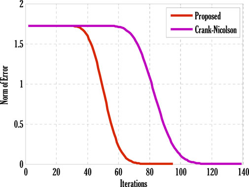
The exact solution to the problem (53)-(55) is $u (t, x) = e^{- t} \sin (x)$ . Equation 53 with boundary and initial conditions (54)–(55) is solved with the existing Crank-Nicolson scheme and proposed scheme. The space discretization is performed with a fourth-order compact scheme. The two schemes are compared in Figure 1. Figure 1 shows the error norm over iterations consumed by both schemes. Since the proposed scheme is more accurate than the existing Crank-Nicolson scheme, it converges faster than the existing scheme using the same step sizes for both schemes.

FIGURE 1

FIGURE 1. Comparison of the proposed scheme with the Crank-Nicolson scheme for the norm of error over iterations using $N^{t} = 190, N^{x} = 45, t_{f} = 1, L = π$ .

Example 5.2:. Casson NanoFluid Flow Over Oscillatory SheetConsider laminar, incompressible, unsteady, and unidirectional mixed convective Casson fluid flow over the oscillatory sheet. Let the sheet be moving with velocity $U_{w} = U_{\circ} \cos (a ω t^{*})$ or $U_{\circ} \sin (a ω t^{*})$ . Let the $x^{*}$ -axis be placed along the plate and $y^{*}$ -axis be placed perpendicular to the plate. Initially, the plate is at rest, and then it starts to move in positive $x^{*}$ -axis. Consider the effects of Joule heating, thermal radiation, and chemical reaction. Under the assumption of boundary layer theory, considering Darcy Forcheimmer’s characteristics and [47], the governing equations of the flow can be expressed as:

\frac{\partial u^{*}}{\partial t^{*}} = ν (1 + \frac{1}{β}) \frac{\partial^{2} u^{*}}{\partial {y^{*}}^{2}} + g (β_{\circ} (T - T_{\infty}) + β_{1} {(T - T_{\infty})}^{2} + β_{2} (C - C_{\infty}) + β_{3} {(C - C_{\infty})}^{2}) - \frac{σ B_{\circ}^{2}}{ρ} u^{*} - \frac{ν}{k_{p}} u^{*} - F {u^{*}}^{2} (56)

\frac{\partial T}{\partial t^{*}} = α \frac{\partial^{2} T}{\partial y^{*^{2}}} + \frac{ν}{C_{p}} (1 + \frac{1}{β}) {(\frac{\partial u^{*}}{\partial y^{*}})}^{2} + \frac{σ B_{\circ}^{2}}{ρ C_{p}} {u^{*}}^{2} + τ (D_{B} \frac{\partial C}{\partial y^{*}} \frac{\partial T}{\partial y^{*}} + \frac{D_{T}}{T_{\infty}} {(\frac{\partial T}{\partial y^{*}})}^{2}) (57)

\frac{\partial C}{\partial t^{*}} = D_{B} \frac{\partial^{2} C}{\partial y^{*^{2}}} + \frac{D_{T}}{T_{\infty}} \frac{\partial^{2} T}{\partial y^{*^{2}}} - k_{1} (C - C_{\infty}), (58)

subject to the boundary conditions,

\begin{array}{c} u^{*} (t^{*}, y^{*}) = U_{o} \cos (a ω t^{*}) o r U_{o} \sin (a ω t^{*}), T (t^{*}, y^{*}) = T_{w}, C (t^{*}, y^{*}) = C_{w} w h e n y^{*} = 0, \\ u^{*} (t^{*}, y^{*}) \to 0, T (T^{*}, y^{*}) \to 0, C (t^{*}, y^{*}) \to 0, w h e n y^{*} \to \infty, \end{array}\} (59)

For reducing Eqs. 55–58 to dimensionless PDEs, the following transformation are considered:

u = \frac{u^{*}}{U_{0}}, y = \sqrt{\frac{ω}{ν}} y^{*}, t = ω t^{*}, θ = \frac{T - T_{\infty}}{T_{w} - T_{\infty}}, ϕ = \frac{C - C_{\infty}}{C_{w} - C_{\infty}} (60)

Under transformations (60), Eqs. 56–59 can be expressed as:

\frac{\partial u}{\partial t} = (1 + \frac{1}{β}) \frac{\partial^{2} u}{\partial y^{2}} - M u - K u - F_{r} u^{2} + λ_{1} θ + λ_{1} μ_{1} θ^{2} + λ_{2} ϕ + λ_{2} μ_{2} ϕ^{2}, (61)

\frac{\partial θ}{\partial t} = \frac{1}{P_{r}} (1 + \frac{4}{3} R_{d}) \frac{\partial^{2} θ}{\partial y^{2}} + E_{c} (1 + \frac{1}{β}) {(\frac{\partial u}{\partial y})}^{2} + M E_{c} u^{2} + N_{b} \frac{\partial θ}{\partial y} \frac{\partial ϕ}{\partial y} + N_{t} {(\frac{\partial θ}{\partial y})}^{2} (62)

\frac{\partial ϕ}{\partial t} = \frac{1}{S_{c}} \frac{\partial^{2} ϕ}{\partial y^{2}} + \frac{1}{S_{c}} \frac{N_{t}}{N_{b}} \frac{\partial^{2} θ}{\partial y^{2}} - γ ϕ (63)

subject to the dimensionless boundary conditions

\begin{array}{c} u (t, y) = \cos (a t) o r \sin (a t), θ (t, y) = 1, ϕ (t, y) = 1 w h e n y = 0, \\ u (t, y) \to 0, θ (t, y) \to 0, ϕ (t, y) \to 0 w h e n y \to \infty . \end{array}\} (64)

The parameters are defined as follows:

λ_{1} = \frac{g β_{\circ} (T_{w} - T_{\infty})}{ω u_{\circ}}, λ_{2} = \frac{g β_{2} (C_{w} - C_{\infty})}{ω u_{\circ}}, M = \frac{σ B_{\circ}^{2}}{ω ρ}, K = \frac{ν}{ω k_{p}}, F_{r} = \frac{c_{b}}{ω k_{p}^{\frac{1}{2}}}, P_{r} = \frac{ν}{α},

R_{d} = \frac{4 σ^{*} T_{\infty}^{3}}{k k^{*}}, E_{c} = \frac{U_{\circ}^{2}}{c_{p} (T_{w} - T_{\infty})}, N_{b} = \frac{τ D_{B} (C_{w} - C_{\infty})}{ν}, N_{t} = \frac{τ D_{T} (T_{w} - T_{\infty})}{ν T_{\infty}}, S_{c} = \frac{ν}{D_{B}}, γ = \frac{k_{1}}{ω}

For solving Eqs. 61–64, the proposed scheme in time direction with fourth-order compact scheme discretization in space is employed. But, the compact scheme requires the computation of a fourth-order spatial partial derivative, which is given as

\frac{\partial^{4} u}{\partial y^{4}} = \frac{1}{1 + \frac{1}{β}} [\frac{\partial^{3} u}{\partial y^{2} \partial t} + M \frac{\partial^{2} u}{\partial y^{2}} + λ \frac{\partial^{2} u}{\partial y^{2}} + F_{r} \bar{u} \frac{\partial^{2} u}{\partial y^{2}} - λ_{1} \frac{\partial^{2} θ}{\partial y^{2}} - λ_{1} μ_{1} \bar{θ} \frac{\partial^{2} θ}{\partial y^{2}} - λ_{2} \frac{\partial^{2} ϕ}{\partial y^{2}} - λ_{2} μ_{2} \bar{ϕ} \frac{\partial^{2} ϕ}{\partial y^{2}}] (65)

Employing the fourth-order scheme to Eq. 61, which yields

{\frac{\partial u}{\partial t}|}_{i} = (1 + \frac{1}{β}) [δ_{y}^{2} u_{i} - \frac{{(Δ y)}^{2}}{12} {\frac{\partial^{4} u}{\partial y^{4}}|}_{i}] - M u_{i} - λ u_{i} - F_{r} \bar{u} u_{i} + λ_{1} θ_{i} + λ_{1} μ_{1} \bar{θ_{i}} θ_{i} + λ_{2} \bar{ϕ} ϕ_{i} + λ_{2} μ_{2} \bar{ϕ} ϕ_{i} (66)

Since the fourth-order spatial derivative is found in Eq. 65, so substituting Eq. 65 into Eq. 66 and the following equation can be obtained

\begin{matrix} \frac{\partial}{\partial t} (u_{i} + \frac{{(Δ y)}^{2}}{12} δ_{y}^{2} u_{i}) = (1 + \frac{1}{β} - \frac{{(Δ y)}^{2}}{12} F_{r} {\bar{u}}_{i} - \frac{{(Δ y)}^{2}}{12} (M + λ)) δ_{y}^{2} u_{i} \\ - (M + λ) u_{i} - F_{r} {\bar{u}}_{i} u_{i} + \frac{{(Δ y)}^{2}}{12} λ_{1} (1 + μ_{1} {\bar{θ}}_{i}) δ_{y}^{2} θ_{i} \\ + \frac{{(Δ y)}^{2}}{12} λ_{2} (1 + μ_{2} {\bar{ϕ}}_{i}) δ_{y}^{2} ϕ_{i} + λ_{1} (1 + μ_{1} {\bar{θ}}_{i}) θ_{i} + λ_{2} (1 + μ_{2} {\bar{ϕ}}_{i}) δ_{y}^{2} ϕ_{i} \end{matrix} (67)

Employing the first stage of the proposed scheme to Eq. 67, which is an explicit scheme, that gives

{\bar{u}}_{i}^{n + 1} + \frac{{(Δ y)}^{2}}{12} δ_{y}^{2} {\bar{u}}_{i}^{n + 1} - u_{i}^{n} - \frac{{(Δ y)}^{2}}{12} δ_{y}^{2} u_{i}^{n} = Δ t H_{i}^{n} (68)

Employing the second stage of the proposed scheme on Eq. 67, which is an implicit stage of the scheme, yields

u_{i}^{n + 1} + \frac{{(Δ y)}^{2}}{12} δ_{y}^{2} u_{i}^{n + 1} - u_{i}^{n} - \frac{{(Δ y)}^{2}}{12} δ_{y}^{2} u_{i}^{n} = Δ t [a_{1} H_{i}^{n + 1} + a_{2} H_{i}^{n} + a_{3} {\bar{H}}_{i}^{n + 1}] + a_{4} (u_{i}^{n + 1} - 2 u_{i}^{n} + u_{i}^{n - 1}) (69)

where

\begin{matrix} H_{i}^{n} = (1 + \frac{1}{β} - \frac{{(Δ y)}^{2}}{12} F_{r} {\bar{u}}_{i}^{n} - \frac{{(Δ y)}^{2}}{12} (M + λ)) δ_{y}^{2} u_{i}^{n} - (M + λ) u_{i}^{n} \\ - F_{r} {\bar{u}}_{i}^{n} u_{i}^{n} + \frac{{(Δ y)}^{2}}{12} λ_{1} (1 + μ_{1} {\bar{θ}}_{i}) δ_{y}^{2} θ_{i}^{n} + \frac{{(Δ y)}^{2}}{12} λ_{2} \\ (1 + μ_{2} {\bar{ϕ}}_{i}^{n}) δ_{y}^{2} ϕ_{i}^{n} + λ_{1} (1 + μ_{1} {\bar{θ}}_{i}^{n}) θ_{i}^{n} + λ_{2} (1 + μ_{1} {\bar{ϕ}}_{i}^{n}) δ_{y}^{2} ϕ_{i}^{n} \end{matrix}

First, employ a compact scheme on Eq. 62 for spatial discretization. The semi-discrete equation can be expressed as

\frac{\partial}{\partial t} [θ_{i} + \frac{{(∆ y)}^{2}}{12} (\begin{array}{c} δ_{y}^{2} θ_{i} + μ δ_{y} u_{i} + \\ μ_{3} δ_{y} θ_{i} \end{array})] = P_{1} δ_{y}^{2} θ_{i} + P_{2} δ_{y}^{2} u_{i} + P_{3} δ_{y} u_{i} + P_{4} δ_{y} θ_{i} + P_{5} δ_{y} ϕ_{i} + M E_{c} {\bar{u}}_{i} u_{i} (70)

where

\begin{matrix} δ = {E_{c} δ}_{y} u_{i}, δ_{1} = E_{c} (1 + \frac{1}{β}) \bar{δ_{y} u_{i}}, δ_{2} = 1 + \frac{1}{β}, δ_{3} \\ = N_{b} \bar{δ_{y} ϕ_{i}} + N_{t} \bar{δ_{y} θ_{i}}, P_{1} = \frac{1}{P_{r}} (1 + \frac{4}{3} R_{d}) + \frac{{(∆ y)}^{2}}{12} δ_{3}, P_{2} \\ = \frac{{(∆ y)}^{2}}{12} M E_{c} {\bar{u}}_{i} + \frac{{(∆ y)}^{2}}{12} δ_{3} (\frac{P_{r}}{1 + \frac{4}{3} R_{d}}) δ_{1}, P_{3} \\ = δ_{1} - \frac{{(∆ y)}^{2}}{12} (M + λ + F_{r} {\bar{u}}_{i}) + \frac{{(∆ y)}^{2}}{12} \frac{δ_{3} P_{r} M E_{c} {\bar{u}}_{i}}{1 + \frac{4}{3} R_{d}}, P_{4} \\ = \frac{{(∆ y)}^{2}}{12} δ λ_{1} + \frac{{(∆ y)}^{2}}{12} δ λ_{1} μ_{1} {\bar{θ}}_{i}, P_{5} = \frac{{(∆ y)}^{2}}{12} δ λ_{2} + \frac{{(∆ y)}^{2}}{12} δ λ_{2} μ_{2} \end{matrix}

For time discretization, applying the first stage of the proposed scheme to Eq. 70, which gives

{\bar{θ}}_{i}^{n + 1} + \frac{{(∆ y)}^{2}}{12} (\begin{array}{c} δ_{y}^{2} {\bar{θ}}_{i}^{n + 1} + δ δ_{y} {\bar{u}}_{i}^{n + 1} + \\ δ_{3} δ_{y} {\bar{θ}}_{i}^{n + 1} \end{array}) - {\bar{θ}}_{i}^{n} - \frac{{(∆ y)}^{2}}{12} (\begin{array}{c} δ_{y}^{2} {\bar{θ}}_{i}^{n} + δ δ_{y} {\bar{u}}_{i}^{n} + \\ δ_{3} δ_{y} {\bar{θ}}_{i}^{n} \end{array}) = Δ t G_{i}^{n} (71)

Employing the second stage of the proposed scheme to Eq. 70 gives

\begin{aligned} θ_{i}^{n + 1} + \frac{{(∆ y)}^{2}}{12} (δ_{y}^{2} θ_{i}^{n + 1} + δ δ_{y} u_{i}^{n + 1} + δ_{3} δ_{y} θ_{i}^{n + 1}) - θ_{i}^{n} - \frac{{(∆ y)}^{2}}{12} (δ_{y}^{2} θ_{i}^{n} + δ δ_{y} u_{i}^{n} + δ_{3} δ_{y} θ_{i}^{n}) \\ = ∆ t \{{a_{1} G}_{i}^{n + 1} + {a_{2} \bar{G}}_{i}^{n + 1} + {a_{3} G}_{i}^{n}\} + a_{4} (θ_{i}^{n + 1} - 2 θ_{i}^{n} + θ_{i}^{n - 1}) \end{aligned} (72)

where

{G_{i}^{n} = P}_{1} δ_{y}^{2} θ_{i}^{n} + P_{2} δ_{y}^{2} u_{i}^{n} + P_{3} δ_{y} u_{i}^{n} + P_{4} δ_{y} θ_{i}^{n} + P_{5} δ_{y} ϕ_{i}^{n} + M E_{c} {\bar{u}}_{i} u_{i}^{n}

For getting a semi-discrete equation, applying a compact scheme to Eq. 63, is obtained

\frac{\partial}{\partial t} [ϕ_{i} + \frac{{(∆ y)}^{2}}{12} δ_{y}^{2} ϕ_{i}] = [\frac{1}{S_{c}} + \frac{{(∆ y)}^{2}}{12} γ] δ_{y}^{2} ϕ_{i} + \frac{1}{S_{c}} \frac{N_{t}}{N_{b}} δ_{y}^{2} θ_{i} - γ ϕ_{i} (73)

To get a fully discrete equation, employing the first stage of the proposed scheme to Eq. 73 and gives

{\bar{ϕ}}_{i}^{n + 1} + \frac{{(∆ y)}^{2}}{12} δ_{y}^{2} {\bar{ϕ}}_{i}^{n + 1} - ϕ_{i}^{n} + \frac{{(∆ y)}^{2}}{12} δ_{y}^{2} ϕ_{i}^{n} = ∆ t F_{i}^{n} (74)

Applying the second implicit stage of the proposed scheme on Eq. 80 gives

ϕ_{i}^{n + 1} + \frac{{(∆ y)}^{2}}{12} δ_{y}^{2} ϕ_{i}^{n + 1} - ϕ_{i}^{n} + \frac{{(∆ y)}^{2}}{12} δ_{y}^{2} ϕ_{i}^{n} = ∆ t [\begin{array}{c} a_{1} F_{i}^{n + 1} + a_{2} {\bar{F}}_{i}^{n + 1} + \\ a_{3} F_{i}^{n} \end{array}] + a_{4} (\begin{array}{c} ϕ_{i}^{n + 1} - 2 ϕ_{i}^{n} + \\ ϕ_{i}^{n - 1} \end{array}) (75)

where

F_{i}^{n} = [\frac{1}{S_{c}} + \frac{{(∆ y)}^{2}}{12} γ] δ_{y}^{2} ϕ_{i}^{n} + \frac{1}{S_{c}} \frac{N_{t}}{N_{b}} δ_{y}^{2} θ_{i}^{n} - γ ϕ_{i}^{n}

System of Eqs. 61–64 is solved using the proposed scheme with third-order accuracy in time. The first stage of the scheme can be applied to solve a given time-dependent parabolic equation without using any other scheme. But the second stage of the scheme requires using any other scheme to find a solution at the first time level. Two types of numerical schemes have been proposed. One of these schemes does not require any other scheme to find a solution at the first time level, but the second scheme requires either some estimated solution or a solution found by any different scheme. Mainly, scheme with higher accuracy converges faster than those having low order accuracy. So, high-order schemes may have been preferred over low-order schemes for finding solutions to parabolic equations with some chosen error norm. Since the proposed schemes are implicit, an additional iterative scheme is chosen for solving difference equation(s) obtained by applying the proposed scheme to given PDE(s). The considered iterative scheme for this contribution is the Gauss-Seidel iterative method. This iterative scheme requires some initial guess to begin finding a solution. The first iteration of the solution is found by considering the initial guess, and later on, the solution is found by utilizing previous consecutive iterations. The iterative procedure will stop if desired criteria are met. The given stopping criteria are based on the maximum norms of solutions for each equation in the system computed at two consecutive iterations. In this contribution, an iterative scheme is considered to solve difference equations obtained by applying the proposed scheme to parabolic equations. This process finds the solution at each grid point and time level. The difference equations can be solved exactly by forming a metric vector equation. But, in this study, only the iterative procedure is considered. Stability is one of the most important factors for getting the converged solution. But, the constructed Matlab code also shows the convergence and divergence of the solution that depends on the numerical values of chosen parameters and values of step sizes in some particular interval.Figure 2 deliberates comparing the proposed scheme with the existing Crank-Nicolson scheme. The maximum of norms for the solution of each Eqs. 61–64 is computed. The norm for the difference between two solutions computed at two consecutive iterations is found, and a maximum of three norms over each iteration is displayed in Figure 2. From this Figure 2, it can be observed that the proposed scheme converges faster than the existing scheme. Since the proposed scheme gives third-order accuracy in time and fourth-order in space, whereas Crank-Nicolson provides second-order accuracy in time and fourth-order in space, it converges faster than the existing scheme. Figs. 3–9 shows the effect of different parameters on velocity, temperature, and concentration profiles obtained by applying the proposed numerical scheme on Eqs. 61–64.Figure 3 shows the effect of the Casson parameter and magnetic parameter on the velocity profile. It is seen that the velocity profile declines by incrementing Casson and magnetic parameters. This fall in velocity profile due to the Casson parameter is the consequence of the diffusion coefficient reduction affecting the flow’s velocity. The rising values of the magnetic parameter diminish the flow’s velocity because the generation of Lorentz force in electrically conducting fluid resists the flow’s velocity, and consequently velocity of the flow drops. The effect of the porosity parameter and inertia coefficient on the flow’s velocity is discussed in Figure 4. Velocity profile de-escalates by enhancing the porosity parameter and inertia coefficient. Since the fluid’s viscosity resists the flow’s velocity, increasing the porosity parameter increases the fluid’s viscosity and reduces the velocity profile. Also, the velocity of the flow de-escalates by enhancing the inertia coefficient; this is the case when the drag force escalates, resulting in a decline in the flow’s velocity. The impact of thermal and solutal mixed convection parameters on the velocity profile is portrayed in Figure 5. Velocity profile rises by augmenting thermal and solutal mixed convection parameters. The rise in the velocity profile results from the temperature and concentration difference growth between the wall and the region away from the plate. Since the rise of temperature and concentration differences produces faster heat and concentration gradients in the flow, for mixed convection problems, temperature and concentration gradients are the factors responsible for generating flow in the fluid. Therefore, the flow’s velocity develops by growing thermal and solutal mixed convection parameters. The effect of the Eckert number and radiation parameter on the temperature profile is discussed in Figure 6. The rising Eckert number and radiation parameter boost the temperature profile. Since the temperature profile is affected by the dissipation due to internal friction of particles in the fluid flow and by improving Eckert number, the temperature profile escalates. Also, due to the entrance of radiations in the flow, heat flux increases; therefore, the temperature profile is boosted. Figure 7 displays the variation of thermophoresis and Brownian motion parameters on the temperature profile. The temperature profile is escalated by uprising thermophoresis and Brownian motion parameters. The increment in the thermophoresis parameter results in the growth of thermophoresis force, due to which heavy particles of fluid come closer to the plate, and lighter particles tend to move from the plate to its surroundings. This procedure of shifting particles improves the temperature of the flow. The boost in the Brownian motion parameter improves the random movement of particles in the fluid; therefore, the temperature profile is boosted. The influence of the Schmidt number and reaction rate parameter on the concentration profile is depicted in Figure 8. Concentration profile is de-escalated by rising Schmidt number and reaction rate parameter values. The increment in the Schmidt number produces low mass diffusivity, resulting in decay in the concentration profile. The augmentation in the reaction rate parameter yields the breaking and forming of particles that slow down the concentration profile. Figure 9 deliberates the variation of thermophoresis and Brownian motion parameters on the concentration profile. The concentration profile escalates by raising the values of the thermophoresis parameter, whereas it de-escalates by increasing the Brownian motion parameter values. Figure 10, Figure 11, Figure 12, Figure 13, Figure 14, Figure 15, Figure 16 show the contour plots of velocity, temperature, and concentration profiles using sine boundary conditions. The variation of the oscillatory boundary can be seen in contour plots of velocity and temperature profiles. Figure 16 shows the comparison of the solution obtained by the proposed scheme with those obtained by the exact solution for solving Stokes’ second problem. The obtained results can be verified by looking at this comparison given in Figure 16.

FIGURE 2

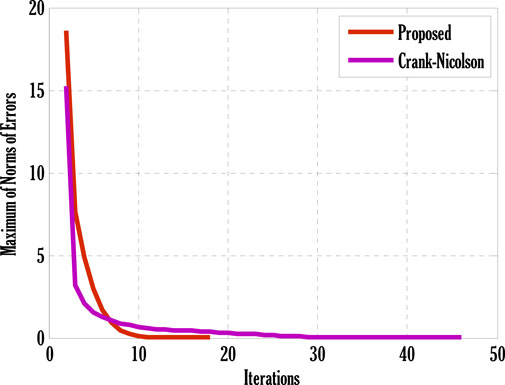
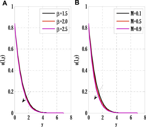
FIGURE 2. Comparison of the proposed scheme with the Crank-Nicolson scheme for finding the maximum norms of errors over iterations using $\begin{matrix} N^{t} = 150, N^{y} = 45, L = 7, t^{f} = 1, E_{c} = 0.5, N_{t} = 0.1, N_{b} = 0.1, P_{r} = 1, S_{c} = 1, \\ R_{d} = 0.25, λ = 0.5, F_{r} = 1.5, λ_{1} = 0.1, μ_{1} = 0.05, λ_{2} = 0.1, μ_{2} = 0.1, γ = 0.9, M = 0.5, β = 3 \end{matrix}$ .

FIGURE 3

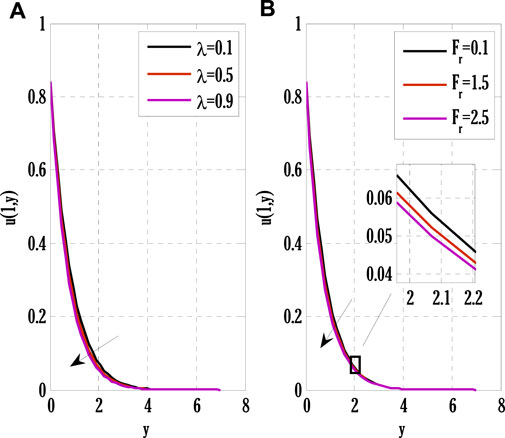
FIGURE 3. Effect of Casson and magnetic parameters on velocity profile using $\begin{matrix} N^{t} = 150, N^{y} = 45, L = 7, t^{f} = 1, E_{c} = 0.9, N_{t} = 0.1, N_{b} = 0.15, P_{r} = 1, S_{c} = 1, \\ R_{d} = 0.1, λ = 0.1, F_{r} = 0.1, λ_{1} = 0.1, μ_{1} = 0.05, λ_{2} = 0.1, μ_{2} = 0.1, γ = 0.9 \end{matrix}$ (A) M = 0.5 (B) β = 3.

FIGURE 4

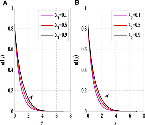
FIGURE 4. Effect of porosity parameter and inertia coefficient on velocity profile using $N^{t} = 150, N^{y} = 45, L = 7, t^{f} = 1, E_{c} = 0.9, N_{t} = 0.1, N_{b} = 0.15, P_{r} = 1, S_{c} = 1, R_{d} = 0.1, M = 0.9, β = 3, λ_{1} = 0.1, μ_{1} = 0.05, λ_{2} = 0.1, μ_{2} = 0.1, γ = 0.9$ (A) F_r = 0.1 (B) λ = 0.1.

FIGURE 5

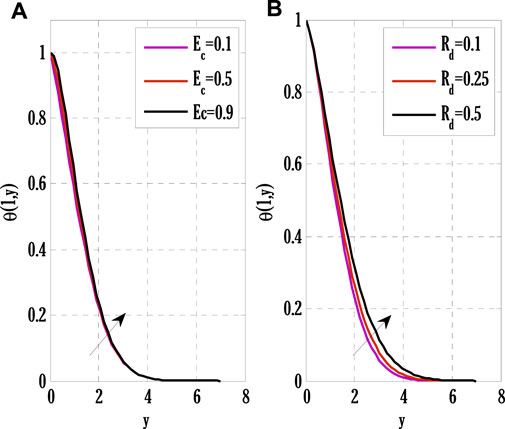
FIGURE 5. Effect of thermal and solutal mixed convection parameters on velocity profile using $N^{t} = 150, N^{y} = 45, L = 7, t^{f} = 1, E_{c} = 0.9, N_{t} = 0.1, N_{b} = 0.15, P_{r} = 1, S_{c} = 1, R_{d} = 0.1, M = 0.9, β = 3, F_{r} = 1.5, μ_{1} = 0.05, λ = 0.5, μ_{2} = 0.1, γ = 0.9$ (A) λ₂ = 0.1 (B) λ₁ = 0.1.

FIGURE 6

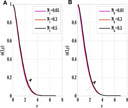
FIGURE 6. Effect of Eckert number and radiation parameters on temperature profile using $N^{t} = 150, N^{y} = 45, L = 7, t^{f} = 1, λ_{1} = 0.1, N_{t} = 0.1, N_{b} = 0.15, P_{r} = 1, S_{c} = 1, λ_{2} = 0.1, M = 0.9, β = 3, F_{r} = 1.5, μ_{1} = 0.05, λ = 0.5, μ_{2} = 0.1, γ = 0.9$ (A) R_d = 0.1 (B) E_C = 0.5.

FIGURE 7

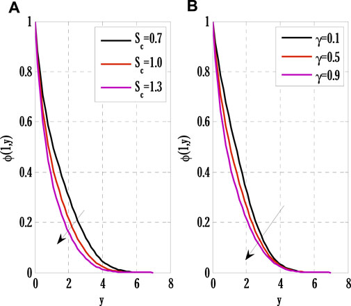
FIGURE 7. Effect of thermophoretic and Brownian motion parameters on temperature profile using $\begin{matrix} N^{t} = 150, N^{y} = 45, L = 7, t^{f} = 1, E_{c} = 0.9, λ_{1} = 0.1, λ_{2} = 0.1, R_{d} = 0.1, \\ P_{r} = 1, S_{c} = 1, R_{d} = 0.1, M = 0.9, β = 3, F_{r} = 1.5, μ_{1} = 0.05, λ = 0.5, μ_{2} = 0.1, γ = 0.9 \end{matrix}$ (A) N_b = 0.15 (B) N_t = 0.1.

FIGURE 8

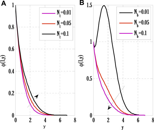
FIGURE 8. Effect of Schmidt number and reaction rate parameter on concentration profile using $\begin{matrix} N^{t} = 150, N^{y} = 45, L = 7, t^{f} = 1, E_{c} = 0.5, R_{d} = 0.25, P_{r} = 1, S_{c} = 1, R_{d} = 0.25, M = 0.5, β = 3, F_{r} = 1.5, \\ μ_{1} = 0.05, λ_{1} = 0.1, λ_{2} = 0.1, λ = 0.5, μ_{2} = 0.1, N_{b} = 0.1, N_{t} = 0.1 \end{matrix}$ (A) γ = 0.9 (B) S_c = 1.

FIGURE 9

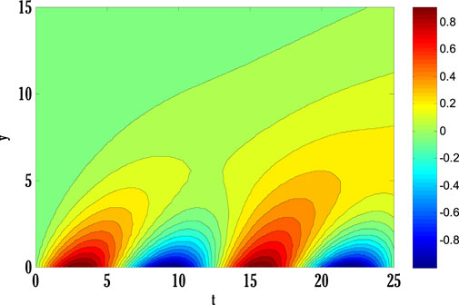
FIGURE 9. Effect of thermophoretic and Brownian motion parameters on concentration profile using $\begin{matrix} N^{t} = 150, N^{y} = 45, L = 7, t^{f} = 1, E_{c} = 0.5, λ_{1} = 0.1, λ_{2} = 0.1, R_{d} = 0.1, P_{r} = 1, S_{c} = 1, R_{d} = 0.25, M = 0.5, β = 3, F_{r} = 1.5, \\ μ_{1} = 0.05, λ = 0.5, μ_{2} = 0.1, γ = 0.9 \end{matrix}$ (A) N_b = 0.1 (B) N_t = 0.1.

FIGURE 10

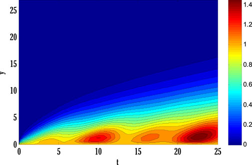
FIGURE 10. Contour plot of velocity profile using $\begin{matrix} N^{t} = 270, N^{y} = 45, L = 27, t^{f} = 1, E_{c} = 01.9, λ_{1} = 0.1, λ_{2} = 0.1, R_{d} = 0.1, P_{r} = 1, S_{c} = 1, R_{d} = 0.1, \\ M = 0.1, β = 2, F_{r} = 0.1, μ_{1} = 0.05, λ = 0.1, μ_{2} = 0.1, γ = 0.9, N_{b} = 0.15, N_{t} = 0.1, u (t, 0) = \sin (0.5 t) \end{matrix}$ .

FIGURE 11

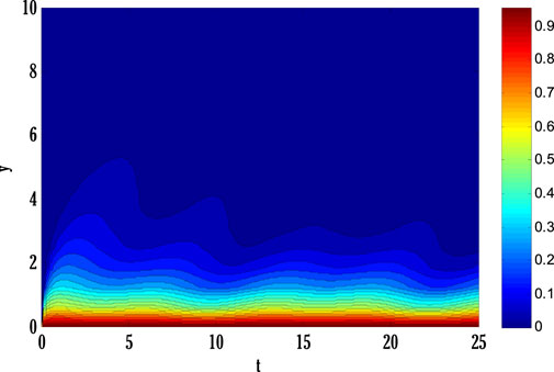
FIGURE 11. Contour plot of temperature profile using $\begin{matrix} N^{t} = 270, N^{y} = 45, L = 27, t^{f} = 1, E_{c} = 01.9, λ_{1} = 0.1, λ_{2} = 0.1, R_{d} = 0.1, P_{r} = 1, S_{c} = 1, R_{d} = 0.1, \\ M = 0.1, β = 2, F_{r} = 0.1, μ_{1} = 0.05, λ = 0.1, μ_{2} = 0.1, γ = 0.9, N_{b} = 0.15, N_{t} = 0.1, u (t, 0) = \sin (0.5 t) \end{matrix}$ .

FIGURE 12

FIGURE 12. Contour plot of concentration profile using $\begin{matrix} N^{t} = 270, N^{y} = 45, L = 27, t^{f} = 1, E_{c} = 01.9, λ_{1} = 0.1, λ_{2} = 0.1, R_{d} = 0.1, P_{r} = 1, S_{c} = 1, R_{d} = 0.1, \\ M = 0.1, β = 2, F_{r} = 0.1, μ_{1} = 0.05, λ = 0.1, μ_{2} = 0.1, γ = 0.9, N_{b} = 0.15, N_{t} = 0.1, u (t, 0) = \sin (0.5 t) \end{matrix}$ .

FIGURE 13

FIGURE 13. Contour plot of velocity profile using $\begin{matrix} N^{t} = 270, N^{y} = 45, L = 27, t^{f} = 1, E_{c} = 01.9, λ_{1} = 0.1, λ_{2} = 0.1, R_{d} = 0.1, P_{r} = 1, S_{c} = 1, R_{d} = 0.1, M = 0.1, \\ β = 2, F_{r} = 0.1, μ_{1} = 0.05, λ = 0.1, μ_{2} = 0.1, γ = 0.9, N_{b} = 0.15, N_{t} = 0.1, u (t, 0) = \sin (3 t) \end{matrix}$ .

FIGURE 14

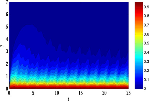
FIGURE 14. Contour plot of temperature profile using $\begin{matrix} N^{t} = 270, N^{y} = 45, L = 27, t^{f} = 1, E_{c} = 01.9, λ_{1} = 0.1, λ_{2} = 0.1, R_{d} = 0.1, P_{r} = 1, S_{c} = 1, R_{d} = 0.1, \\ M = 0.1, β = 2, F_{r} = 0.1, μ_{1} = 0.05, λ = 0.1, μ_{2} = 0.1, γ = 0.9, N_{b} = 0.15, N_{t} = 0.1, u (t, 0) = \sin (3 t) \end{matrix}$ .

FIGURE 15

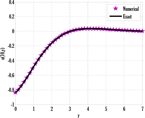
FIGURE 15. Contour plot of concentration profile using $\begin{matrix} N^{t} = 270, N^{y} = 45, L = 27, t^{f} = 1, E_{c} = 01.9, λ_{1} = 0.1, λ_{2} = 0.1, R_{d} = 0.1, P_{r} = 1, S_{c} = 1, R_{d} = 0.1, \\ M = 0.1, β = 2, F_{r} = 0.1, μ_{1} = 0.05, λ = 0.1, μ_{2} = 0.1, γ = 0.9, N_{b} = 0.15, N_{t} = 0.1, u (t, 0) = \sin (3 t) \end{matrix}$ .

FIGURE 16

FIGURE 16. Comparison of the proposed scheme with the exact solution for Stokes׳ second problem.

6 Conclusion

This contribution dealt with numerical schemes for time discretization of time-dependent PDEs. Two schemes have been proposed with third-order accuracy in time. According to von Neumann’s stability analysis and convergence of obtained solution from Matlab code, the scheme was conditionally stable. Moreover, a mathematical model for boundary layer Casson nanofluid flow over an oscillatory sheet has been constructed, influencing joule heating and chemical reaction. The dimensionless form of the model was solved with existing and proposed schemes. An iterative scheme was also adopted to solve discretized or difference equations obtained by proposing a scheme on the considered system of ODEs. Following this research, different applications for the current approach may be developed [48–52]. The main concluding points can be expressed as.

1) The proposed scheme converged faster than the existing Crank-Nicolson scheme.

2) Results have been validated for the velocity profile of the boundary layer flow phenomenon.

3) The velocity profile was decayed by enhancing Casson and magnetic parameters, and growing porosity parameter and inertia coefficient values inclined it.

4) Increasing values of thermophoresis and Brownian motion parameters raised the temperature profile.

5) The concentration profile was escalated by incrementing the thermophoresis parameter.

Data availability statement

The original contributions presented in the study are included in the article/supplementary material, further inquiries can be directed to the corresponding author.

Author contributions

Conceptualization, methodology, and analysis, YN; funding acquisition, WS; investigation, YN; methodology, MM; project administration, KA; resources, KA; supervision, MA.; visualization, KA; writing—review and editing, MA.; proofreading and editing, MM All authors have read and agreed to the published version of the manuscript.

Acknowledgments

The authors wish to express their gratitude to Prince Sultan University for facilitating the publication of this article through the Theoretical and Applied Sciences Lab.

Conflict of interest

The authors declare that the research was conducted in the absence of any commercial or financial relationships that could be construed as a potential conflict of interest.

Publisher’s note

All claims expressed in this article are solely those of the authors and do not necessarily represent those of their affiliated organizations, or those of the publisher, the editors and the reviewers. Any product that may be evaluated in this article, or claim that may be made by its manufacturer, is not guaranteed or endorsed by the publisher.

References

1. Tagawa T. Numerical analysis of magnetohydrodynamic flows. Fluids (2020) 5(1):23. doi:10.3390/fluids5010023

CrossRef Full Text | Google Scholar

2. Miura H. Extended magnetohydrodynamic simulations of decaying, homogeneous, approximately-isotropic and incompressible turbulence. Fluids (2019) 4:46 Accessed March 11, 2019. doi:10.3390/fluids4010046

CrossRef Full Text | Google Scholar

3. Nazeer M, Saleem S, Hussain F, Zia Z, Khalid K, Feroz N. Heat transmission in a magnetohydrodynamic multiphase flow induced by metachronal propulsion through porous media with thermal radiation. Proc Inst Mech Eng E: J Process Mech Eng (2022) 095440892210752. doi:10.1177/09544089221075299

CrossRef Full Text | Google Scholar

4. Bhattacharyya K. Dual solutions in boundary layer stagnation-point flow and mass transfer with chemical reaction past a stretching/shrinking sheet. Int Commun Heat Mass Transfer (2011) 38:917–22. doi:10.1016/j.icheatmasstransfer.2011.04.020

CrossRef Full Text | Google Scholar

5. Bhattacharyya K. Dual solutions in unsteady stagnation-point flow over a shrinking sheet. Chin Phys Lett (2011) 28:084702. doi:10.1088/0256-307x/28/8/084702

CrossRef Full Text | Google Scholar

6. Bhattacharyya K. MHD stagnation-point flow of Casson fluid and heat transfer over a stretching sheet with thermal radiation. J thermodynamics (2013) 2013:1–9. doi:10.1155/2013/169674

CrossRef Full Text | Google Scholar

7. Bhattacharyya K. Heat transfer analysis in unsteady boundary layer stagnation-point flow towards a shrinking/stretching sheet. Ain Shams Eng J (2013) 4:259–64. doi:10.1016/j.asej.2012.07.002

CrossRef Full Text | Google Scholar

8. Bhattacharyya K, Mukhopadhyay S, Layek G. Slip effects on an unsteady boundary layer stagnation-point flow and heat transfer towards a stretching sheet. Chin Phys Lett (2011) 28:094702. doi:10.1088/0256-307x/28/9/094702

CrossRef Full Text | Google Scholar

9. You X, Xu H, Liao S. On the nonsimilarity boundary-layer flows of second-order fluid over a stretching sheet. J Appl Mech (2010) 77:021002. doi:10.1115/1.3173764

CrossRef Full Text | Google Scholar

10. Liao S-J. A general approach to get series solution of non-similarity boundary-layer flows. Commun Nonlinear Sci Numer Simulation (2009) 14:2144–59. doi:10.1016/j.cnsns.2008.06.013

CrossRef Full Text | Google Scholar

11. Nakhchi ME, Nobari M, Tabrizi HB. Non-similarity thermal boundary layer flow over a stretching flat plate. Chin Phys Lett (2012) 29:104703. doi:10.1088/0256-307x/29/10/104703

CrossRef Full Text | Google Scholar

12. Kousar N, Liao S. Series solution of non-similarity natural convection boundary-layer flows over permeable vertical surface. Sci China Phys Mech Astron (2010) 53:360–8. doi:10.1007/s11433-010-0124-z

CrossRef Full Text | Google Scholar

13. Kousar N, Mahmood R. Series solution of non-similarity boundary-layer flow in porous medium. Appl Math (2013) 4. doi:10.4236/am.2013.48A018

CrossRef Full Text | Google Scholar

14. Hunegnaw D, Kishan N. Unsteady MHD heat and mass transfer flow over stretching sheet in porous medium with variable properties considering viscous dissipation and chemical reaction. Chem Sci Int J (2014) 4:901–17. doi:10.9734/acsj/2014/11972

CrossRef Full Text | Google Scholar

15. Chu Y-M, Nazir U, Sohail M, Selim MM, Lee J-R. Enhancement in thermal energy and solute particles using hybrid nanoparticles by engaging activation energy and chemical reaction over a parabolic surface via finite element approach. Fractal and Fractional (2021) 5:119. doi:10.3390/fractalfract5030119

CrossRef Full Text | Google Scholar

16. Abbas S. Z., Nayak M. K., Mabood F., Dogonchi A. S., Chu Y. M., Khan W. A. Darcy Forchheimer electromagnetic stretched flow of carbon nanotubes over an inclined cylinder: Entropy optimization and quartic chemical reaction. Math Methods Appl Sci (2020) 1–23. doi:10.1002/mma.6956

CrossRef Full Text | Google Scholar

17. Liu C, Khan MU, Ramzan M, Chu Y-M, Kadry S, Malik MY, et al. Nonlinear radiative Maxwell nanofluid flow in a Darcy–Forchheimer permeable media over a stretching cylinder with chemical reaction and bioconvection. Scientific Rep (2021) 11:9391. doi:10.1038/s41598-021-88947-5

CrossRef Full Text | Google Scholar

18. Al-Zubaidi A., Nazeer M., Subia G. S., Hussain F., Saleem S., Ghafar M. M. Mathematical modeling and simulation of MHD electro-osmotic flow of Jeffrey fluid in convergent geometry. Waves in Random and Complex Media (2021) 1–17. doi:10.1080/17455030.2021.2000672

CrossRef Full Text | Google Scholar

19. Nazeer M, Hussain F, Khan MI, El-Zahar ER, Chu Y-M, Malik M, et al. Retracted: Theoretical study of MHD electro-osmotically flow of third-grade fluid in micro channel. Appl Math Comput (2022) 420:126868. doi:10.1016/j.amc.2021.126868

CrossRef Full Text | Google Scholar

20. Nazeer M, Hussain F, Shabbir L, Saleem A, Khan MI, Malik M, et al. A comparative study of MHD fluid-particle suspension induced by metachronal wave under the effects of lubricated walls. Int J Mod Phys B (2021) 35:2150204. doi:10.1142/s0217979221502040

CrossRef Full Text | Google Scholar

21. Ali N, Nazeer M, Javed T, Razzaq M. Finite element analysis of bi-viscosity fluid enclosed in a triangular cavity under thermal and magnetic effects. The Eur Phys J Plus (2019) 134:2–20. doi:10.1140/epjp/i2019-12448-x

CrossRef Full Text | Google Scholar

22. Kumar A, Sugunamma V, Sandeep N. Impact of nonlinear radiation on MHD non-aligned stagnation point flow of micropolar fluid over a convective surface. J Non-Equilibrium Thermodynamics (2018) 43:327–45. doi:10.1515/jnet-2018-0022

CrossRef Full Text | Google Scholar

23. Pramanik S. Casson fluid flow and heat transfer past an exponentially porous stretching surface in presence of thermal radiation. Ain Shams Eng J (2014) 5:205–12. doi:10.1016/j.asej.2013.05.003

CrossRef Full Text | Google Scholar

24. Khan MI, Waqas H, Khan SU, Imran M, Chu Y-M, Abbasi A, et al. Slip flow of micropolar nanofluid over a porous rotating disk with motile microorganisms, nonlinear thermal radiation and activation energy. Int Commun Heat Mass Transfer (2021) 122:105161. doi:10.1016/j.icheatmasstransfer.2021.105161

CrossRef Full Text | Google Scholar

25. Qayyum S, Khan MI, Masood F, Chu YM, Kadry S, Nazeer M. Interpretation of entropy generation in Williamson fluid flow with nonlinear thermal radiation and first-order velocity slip. Math Methods Appl Sci (2021) 44:7756–65. doi:10.1002/mma.6735

CrossRef Full Text | Google Scholar

26. Song Y-Q, Khan SA, Imran M, Waqas H, Khan SU, Khan MI, et al. Applications of modified Darcy law and nonlinear thermal radiation in bioconvection flow of micropolar nanofluid over an off centered rotating disk. Alexandria Eng J (2021) 60:4607–18. doi:10.1016/j.aej.2021.03.053

CrossRef Full Text | Google Scholar

27. Waqas H, Khan SA, Khan SU, Khan MI, Kadry S, Chu Y-M. Falkner-Skan time-dependent bioconvrction flow of cross nanofluid with nonlinear thermal radiation, activation energy and melting process. Int Commun Heat Mass Transfer (2021) 120:105028. doi:10.1016/j.icheatmasstransfer.2020.105028

CrossRef Full Text | Google Scholar

28. Alaidrous AA, Eid MR. 3-D electromagnetic radiative non-Newtonian nanofluid flow with Joule heating and higher-order reactions in porous materials. Scientific Rep (2020) 10(1):14513–9. doi:10.1038/s41598-020-71543-4

PubMed Abstract | CrossRef Full Text | Google Scholar

29. Hafeez A, Khan M, Ahmed A, Ahmed J. Features of Cattaneo-Christov double diffusion theory on the flow of non-Newtonian Oldroyd-B nanofluid with Joule heating. Appl Nanoscience (2021) 1–8:265–72. doi:10.1007/s13204-020-01600-x

PubMed Abstract | CrossRef Full Text | Google Scholar

30. Khan A, Shah Z, Alzahrani E, Islam S. Entropy generation and thermal analysis for rotary motion of hydromagnetic Casson nanofluid past a rotating cylinder with Joule heating effect. Int Commun Heat Mass Transfer (2020) 119:104979. doi:10.1016/j.icheatmasstransfer.2020.104979

CrossRef Full Text | Google Scholar

31. Kumar A, Tripathi R, Singh R, &Chaurasiya VK. Simultaneous effects of nonlinear thermal radiation and Joule heating on the flow of Williamson nanofluid with entropy generation. Physica A: Stat Mech its Appl (2020) 551:123972. doi:10.1016/j.physa.2019.123972

CrossRef Full Text | Google Scholar

32. Khashi’ie NS, Arifin NM, Pop I, Wahid NS. Flow and heat transfer of hybrid nanofluid over a permeable shrinking cylinder with joule heating: A comparative analysis. Alexandria Eng J (2020) 59(3):1787–98. doi:10.1016/j.aej.2020.04.048

CrossRef Full Text | Google Scholar

33. Uddin I, Ullah I, Ali R, Khan I, Nisar KS. Numerical analysis of nonlinear mixed convective MHD chemically reacting flow of Prandtl–Eyring nanofluids in the presence of activation energy and Joule heating. J Therm Anal Calorim (2021) 145(2):495–505. doi:10.1007/s10973-020-09574-2

CrossRef Full Text | Google Scholar

34. Kazemi MA, Javanmard M, Taheri MH, Askari N. Heat transfer investigation of the fourthgrade non-Newtonian MHD fluid flow in a plane duct considering the viscous dissipation, joule heating and forced convection on the walls. SN Appl Sci (2020) 2(10):1752–14. doi:10.1007/s42452-020-03567-4

CrossRef Full Text | Google Scholar

35. Ur Rasheed H, Saleem S, Islam S, Khan Z, Khan W, Firdous H, et al. Effects of joule heating and viscous dissipation on magnetohydrodynamic boundary layer flow of jeffrey nanofluid over a vertically stretching cylinder. Coatings (2021) 11(3):353. doi:10.3390/coatings11030353

CrossRef Full Text | Google Scholar

36. Eswaramoorthi S, Loganathan K, Faisal M, Botmart T, Shah NA. Analytical and numerical investigation of Darcy-Forchheimer flow of a nonlinear-radiative non-Newtonian fluid over a Riga plate with entropy optimization. Ain Shams Eng J (2022) 14:101887. doi:10.1016/j.asej.2022.101887

CrossRef Full Text | Google Scholar

37. Rasool G, Shah NA, El-Zahar ER, Wakif A. Numerical investigation of EMHD nanofluid flows over a convectively heated riga pattern positioned horizontally in a Darcy-forchheimer porous medium: Application of passive control strategy and generalized transfer laws. Waves in Random and Complex Media (2022).

CrossRef Full Text | Google Scholar

38. Rauf A, Shah NA, Mushtaq A, Botmart T. Heat transport and magnetohydrodynamic hybrid micropolar ferrofluid flow over a non-linearly stretching sheet. AIMS Math (2023) 8(1):1–20. doi:10.1080/17455030.2022.2074571

CrossRef Full Text | Google Scholar

39. Wakif A, Shah NA. Hydrothermal and mass impacts of azimuthal and transverse components of Lorentz forces on reacting Von Kármán nanofluid flows considering zero mass flux and convective heating conditions. Waves in Random and Complex Media (2022) 1–22.

CrossRef Full Text | Google Scholar

40. Shah NA, Asogwa KK, Mahsud Y, Lee SR, Kang S, Chung JD, et al. Effect of generalized thermal transport on MHD free convection flows of nanofluids: A generalized atangana-baleanu derivative model. Case Stud Therm Eng (2022) 40:102480. doi:10.1080/17455030.2022.2136413

CrossRef Full Text | Google Scholar

41. Zubair Akbar Qureshi M, Faisal M, Raza Q, Ali B, Botmart T, Shah NA. Morphological nanolayer impact on hybrid nanofluids flow due to dispersion of polymer/CNT matrix nanocomposite material. AIMS Math (2023) 8(1):633–56. doi:10.3934/math.2023030

CrossRef Full Text | Google Scholar

42. Ibrahim A. Eigenvalue approach on fractional order theory of thermoelastic diffusion problem for an infinite elastic medium with a spherical cavity. Appl Math Model (2015) 39(20):6196–206. doi:10.1016/j.apm.2015.01.065

CrossRef Full Text | Google Scholar

43. Abbas IA, Zenkour AM. Dual-phase-lag model on thermoelastic interactions in a semi-infinite medium subjected to a ramp-type heating. J Comput Theor Nanoscience (2014) 11(34):642–5. doi:10.1166/jctn.2014.3407

CrossRef Full Text | Google Scholar

44. Priyadharshini P, Archana MV, Ahammad NA, Raju CSK, Yook SJ, Shah NA. Gradient descent machine learning regression for MHD flow: Metallurgy process. Int Commun Heat Mass Transfer (2022) 138:106307. doi:10.1016/j.icheatmasstransfer.2022.106307

CrossRef Full Text | Google Scholar

45. Sajjan K, Shah NA, Ahammad NA, Raju CSK, Kumar MD, Weera W. Nonlinear Boussinesq and Rosseland approximations on 3D flow in an interruption of Ternary nanoparticles with various shapes of densities and conductivity properties. AIMS Math (2022) 7(10):18416–49. doi:10.3934/math.20221014

CrossRef Full Text | Google Scholar

46. Zhang KZ, Shah NA, Vieru D, El-Zahar ER. Memory effects on conjugate buoyant convective transport of nanofluids in annular geometry: A generalized Cattaneo law of thermal flux. Int Commun Heat Mass Transfer (2022) 135:106138. doi:10.1016/j.icheatmasstransfer.2022.106138

CrossRef Full Text | Google Scholar

47. Prabhakar Reddy B, Makinde OD, Hugo A. A computational study on diffusion-thermo and rotation effects on heat generated mixed convection flow of MHD Casson fluid past an oscillating porous plate. Int Commun Heat Mass Transfer (2022) 138:138 106389. doi:10.1016/j.icheatmasstransfer.2022.106389

CrossRef Full Text | Google Scholar

48. Nawaz Y, Shoaib Arif M, Abodayeh K. An explicit-implicit numerical scheme for time fractional boundary layer flows. Int J Numer Methods Fluids (2022) 94:920. Wiley. doi:10.1002/fld.5078

CrossRef Full Text | Google Scholar

49. Shoaib Arif M, Abodayeh K, Nawaz Y. The modified finite element method for heat and mass transfer of unsteady reacting flow with mixed convection. Front Media S.A. (2022) 10:952787. doi:10.3389/fphy.2022.952787

CrossRef Full Text | Google Scholar

50. Nawaz Y, Arif MS, Shatanawi W, Nazeer A. An explicit fourth-order compact numerical scheme for heat transfer of boundary layer flow. Energies (2021) 14(12):3396. doi:10.3390/en14123396

CrossRef Full Text | Google Scholar

51. Shatanawi W, Raza A, Arif MS, Rafiq M, Bibi M, Mohsin M. Essential features preserving dynamics of stochastic Dengue model. Comp Model Eng Sci (2021) 126(1):201–15. doi:10.32604/cmes.2021.012111

CrossRef Full Text | Google Scholar

52 Arif MS, Raza A, Rafiq M, Bibi M, Abbasi JN, Nazeer A, Javed U. Numerical simulations for stochastic computer virus propagation model. Comput. Mater. Contin (2020) 62:61–77. doi:10.32604/cmc.2020.08595

CrossRef Full Text | Google Scholar

Nomenclature

$u^{*}$ Horizontal components of velocity $(m . s^{- 1})$

$σ$ Electrical conductivity of the fluid $(S . m^{- 1})$

$y^{*}$ Cartesian co-ordinate $(m)$

$T$ Temperature of fluid $(K)$

$ν$ Kinematic viscosity $(m^{2} . s^{- 1})$

$T_{w}$ Temperature of fluid at the wall $(K)$

$ρ$ Density of fluid $(k g . m^{- 3})$

$T_{\infty}$ Ambient temperature of the fluid $(K)$

$C$ Concentration of fluid $(m o l . m^{- 3})$

$C_{w}$ Concentration on the wall $(m o l . m^{- 3})$

$D_{B}$ Brownian diffusion coefficient $(m^{2} . s^{- 1})$

$C_{\infty}$ Ambient concentration $(m o l . m^{- 3})$

$c_{p}$ specific heat capacity $(J . {k g}^{- 1} . K^{- 1})$

$D_{T}$ Thermophoresis coefficient $(m^{2} . s^{- 1})$

$E_{0}$ Strength of electric field $(V . m^{- 1})$

$B_{0}$ Strength of imposed transverse magnetic field $(G a u s s m e t e r)$

$k_{p}$ Permeability of porous medium $(m^{2})$

$α$ Thermal diffusivity $(m^{2} . s^{- 1})$

$k_{1}$ Reaction rate parameter $(s^{- 1})$

$c_{b}$ Drag coefficient

$k^{*}$ mean absorption coefficient $(m^{- 1})$

$σ^{*}$ Stephan-Boltzmann constant $(W . m^{- 2} . K^{- 4})$

$β$ Casson parameter

$μ$ Dynamic viscosity $(k g . m^{- 1} . s^{- 1})$

$M$ Magnetic parameter

$β_{1}$ Linear thermal expansion coefficient $(K^{- 1})$

$β_{3}$ Linear solutal expansion coefficient ${(m o l . m^{- 3})}^{- 1}$

$β_{2}$ Non-linear thermal expansion coefficient $(K^{- 2})$

$β_{4}$ Non-linear solutal expansion coefficient ${(m o l . m^{- 3})}^{- 2}$

$E_{c}$ Eckert number

$μ_{1}$ Thermal non-linear convection parameter

$μ_{2}$ Solutal non-linear convection parameter

$F_{r}$ Forchheimer number

$λ$ Permeability of the porous medium

$N_{b}$ Brownian motion variable

$N_{t}$ Thermophoresis variable

$R_{d}$ Radiation parameter

$S_{c}$ Schmidt number

$γ$ Reaction rate

$P_{r}$ Prandtl number

$λ_{1}$ Thermal mixed convection parameter

$λ_{2}$ Solutal mixed convection parameter

$τ$ Effective heat capacity of fluid

Keywords: numerical schemes for ODEs, stability, casson fluid flow, joule heating and numerical solution, convergence and extension

Citation: Nawaz Y, Arif MS, Abodayeh K and Mansoor M (2023) Finite difference schemes for MHD mixed convective Darcy–forchheimer flow of Non-Newtonian fluid over oscillatory sheet: A computational study. Front. Phys. 11:1072296. doi: 10.3389/fphy.2023.1072296

Received: 17 October 2022; Accepted: 09 January 2023;
Published: 02 February 2023.

Edited by:

Antonio F. Miguel, University of Evora, Portugal

Reviewed by:

Nehad Ali Shah, Sejong University, Republic of Korea
Aatef Hobiny, King Abdulaziz University, Saudi Arabia

Copyright © 2023 Nawaz, Arif, Abodayeh and Mansoor. This is an open-access article distributed under the terms of the Creative Commons Attribution License (CC BY). The use, distribution or reproduction in other forums is permitted, provided the original author(s) and the copyright owner(s) are credited and that the original publication in this journal is cited, in accordance with accepted academic practice. No use, distribution or reproduction is permitted which does not comply with these terms.

*Correspondence: Muhammad Shoaib Arif, marif@psu.edu.sa

ORIGINAL RESEARCH article

Finite difference schemes for MHD mixed convective Darcy–forchheimer flow of Non-Newtonian fluid over oscillatory sheet: A computational study

1 Introduction

2 Numerical scheme

3 Stability analysis

4 Problem formulation

5 Numerical examples

6 Conclusion

Data availability statement

Author contributions

Acknowledgments

Conflict of interest

Publisher’s note

References

Nomenclature

People also looked at