 Reetik Kumar Sahu1
 Juliane Müller1*
 Jangho Park1
 Charuleka Varadharajan2
 Bhavna Arora2
 Boris Faybishenko2Deborah Agarwal3
- 1Lawrence Berkeley National Laboratory, Computational Research Division, Center for Computational Sciences and Engineering, Berkeley, CA, United States
- 2Lawrence Berkeley National Laboratory, Earth and Environmental Sciences Area, Berkeley, CA, United States
- 3Lawrence Berkeley National Laboratory, Data Science and Technology, Computational Research Division, Berkeley, CA, United States
With the growing use of machine learning (ML) techniques in hydrological applications, there is a need to analyze the robustness, performance, and reliability of predictions made with these ML models. In this paper we analyze the accuracy and variability of groundwater level predictions obtained from a Multilayer Perceptron (MLP) model with optimized hyperparameters for different amounts and types of available training data. The MLP model is trained on point observations of features like groundwater levels, temperature, precipitation, and river flow in various combinations, for different periods and temporal resolutions. We analyze the sensitivity of the MLP predictions at three different test locations in California, United States and derive recommendations for training features to obtain accurate predictions. We show that the use of all available features and data for training the MLP does not necessarily ensure the best predictive performance at all locations. More specifically, river flow and precipitation data are important training features for some, but not all locations. However, we find that predictions made with MLPs that are trained solely on temperature and historical groundwater level measurements as features, without additional hydrological information, are unreliable at all locations.
Introduction
Groundwater is an important source of freshwater, accounting for almost 38% of the global irrigation demand (Siebert et al., 2010). With growing economies and increasing food demand, the stress on freshwater aquifers has increased in places like North America and Asia (Aeschbach-Hertig and Gleeson, 2012). This situation is further aggravated by increased climate variability. In California, USA, groundwater provides nearly 40% of the water used by the state's cities and farms. Many of the state's groundwater basins have experienced long-term overdraft due to withdrawal rates exceeding recharge rates. The negative impacts of long-term overdraft include higher energy requirements for pumping water from deeper wells, land subsidence, reduced river flow, and impaired water quality (especially in coastal aquifers due to saltwater intrusion). Thus, in 2014, following a series of droughts, the Sustainable Groundwater Management Act (SGMA) was passed, requiring local agencies to sustainably manage groundwater and minimize undesirable results (DWR, 2020). This in turn requires decision makers access to accurate, reliable, and timely predictions of groundwater levels.
Traditionally, groundwater depths and other water budget components such as runoff and soil moisture are estimated using mechanistic multi-scale, multi-physics simulation models such as MODFLOW, PARFLOW, HydroGeoSphere, and TOUGH (Xu et al., 2011; Steefel et al., 2015; Langevin et al., 2017). These models capture physical processes of mass, momentum, and energy transfer through partial differential equations and require extensive characterization of hydrostratigraphic properties and accurate boundary conditions, including recharge sources, climate variability and changes in water use (Sahoo et al., 2017). Such information is not always known a priori, and some parameters can only be determined by solving an inverse problem (Arora et al., 2011), which itself requires running simulation models repeatedly until their values have been determined, thereby substantially increasing the computational costs (Arora et al., 2012). In addition, running the high-fidelity simulation models at high resolution requires high performance computing resources. Therefore, it is difficult for groundwater sustainability agencies and policy makers to use these simulations to guide water management decisions.
With the improvement of sensor technologies and data systems, an unprecedented amount of environmental data are being collected, through established long-term monitoring networks, including river flow, groundwater level, water quality, temperature, and precipitation (Rode et al., 2016). This has resulted in an increased interest in applying ML methods for hydrological applications (Deka, 2014; Shen, 2018) such as river flow forecasts (Lin et al., 2006; Rasouli et al., 2012; Deo and Sahin, 2016; Kratzert et al., 2018); water quality estimation and prediction (Ahmad et al., 2010; Najah et al., 2013; Xu and Liu, 2013), and water demand forecasts (Ghiassi et al., 2008; Herrera et al., 2010; Adamowski et al., 2012; Tiwari and Adamowski, 2013).
Deep learning (DL) models can be trained to approximate the behavior of a complex system, such as a groundwater basin, in a computationally inexpensive way while making highly accurate predictions. DL techniques can utilize the climate and hydrogeology data to capture the relationships between groundwater levels and other dependent features such as nearby river flow, precipitation and temperature. Recent advances in ML have enabled making groundwater predictions by using purely data-driven models (Taormina et al., 2012; Moosavi et al., 2013; Sahoo et al., 2017; Müller et al., 2020). ML techniques have been used for both prediction and optimization purposes including modeling of groundwater levels and or quality, optimization of groundwater well design, pumping rate, and location (Banerjee et al., 2011; Gaur et al., 2013). As an example, Sahoo et al. (2017) utilized a hybrid feedforward neural network (FNN) to model groundwater level changes in the High Plains aquifer, United States, using both in-situ and remote measurements with model simulations of different input features (climate and anthropogenic). Their DL models were trained on monthly data spanning over 33 years. Emamgholizadeh et al. (2014) built a groundwater prediction model using an FNN model built from 9 years of monthly data that included rainfall recharge, pumping rate and irrigated return flow at the Bastam Plain, Iran. The FNN model showed the highest accuracy when built with a lag time of 2 months giving a prediction error of about 3% of difference between observed maximum and minimum levels. Guzman et al. (2017) utilized a dynamic form of a Recurrent Neural Network (RNN) model to predict groundwater levels in the Mississippi River Valley Alluvial aquifer, United States. Eight years of daily historical input time series including precipitation and groundwater levels were used to forecast groundwater levels for up to 3 months. Their results showed that models generated with 100 lag days provided the most accurate prediction of groundwater levels. Adamowski and Chan (2011) coupled discrete wavelet transforms (WA) and artificial neural networks (ANN) to predict groundwater levels using monthly average precipitation, temperature, and groundwater level at two sites in the Chateauguay watershed in Quebec, Canada. Their WA-ANN models performed better than standard autoregressive integrated moving average (ARIMA) time series models.
All of these prior studies involved building the DL model to predict groundwater levels at a single well. In contrast, Mohanty et al. (2015) built an FNN model to predict weekly groundwater levels simultaneously at 18 different locations in the Mahanadi Delta, India. The input features in this study included weekly values of precipitation, pumping from tubewells, and the river stage. The DL model could predict groundwater levels up to 4 weeks of lead time with a prediction error of about 8% of the annual groundwater-level change. Our previous study (Müller et al., 2020) compared results from a variety of DL methods including multilayer perceptron (MLP), RNN, long short term memory (LSTM), and 1D-convolutional neural network (CNN) designed with our hyperparameter optimization approach for both single- and multi-well groundwater level predictions in California, and were able to attain prediction accuracies of 6–20%, depending on the DL model.
Each of the referenced applications utilize different ML models and architecture under different scenarios such as multi-point vs. single-point sites, with data of varying temporal resolutions (hourly, daily, weekly, and monthly). Despite these differences, and the constraints imposed by data availability, all of these models have similar ranges for prediction accuracies. This raises the following questions: What is the right DL model to use? How should the parameters of the model be tuned? What data should we use to build an accurate prediction model? Most importantly, in order to use DL models effectively to make reliable future groundwater predictions in a computationally inexpensive manner, we must first understand which input features are necessary and sufficient. Additionally, these prior studies only report results from a single optimized neural network, and they do not address the inherent stochasticity that arises during training when using stochastic gradient descent (Amari, 1993). Thus, when training the DL model for the same architecture multiple times, we obtain different performances, and therefore different future predictions. In order to ensure the reliability of the DL model predictions, we must report confidence intervals, as well as average, best, and worst-case predictions. These uncertainty estimates will enable water managers to analyze and explore a wide spectrum of sustainable management practices and to identify those that are the most robust for all scenarios.
To address this critical need, we conduct a critical analysis of the sensitivity of DL model predictions to the choice of input features used to train a model. In particular, we compare the sensitivity of groundwater predictions to different choices of input features including groundwater levels, temperature, precipitation, and river flow. This kind of analysis will extend our understanding of the applicability of ML techniques for hydrological predictions and provide guidance on how to build accurate and reliable models. These DL models can potentially enable water managers to better prepare and sustainably manage water resources in the face of future climate variability.
The remainder of this article is organized as follows. In section Description of Numerical Study, we provide details of the setup for our numerical experiments (including the data collection, processing, and model framework), and present their results in section Numerical Results. In section Discussion, we discuss the results of the numerical experiments in the context of applying ML techniques to groundwater and outline potential future research directions. Finally, in section Conclusion, we present the conclusions of our study.
Description of Numerical Study
In this section, we describe the setup of our numerical experiments, including the data we used, model selection and hyperparameters, our experimental setup for sensitivity analysis, and the method for computing confidence intervals.
Data Collection and Preparation
We focused our study on wells in three different locations in Northern California, United States in Butte County, Shasta County, and Tehama County with different hydrostratigraphy and land use (Figure 1). Moreover, they represent different SGMA basin prioritization categories (high, medium, and low respectively), which are determined by historical groundwater trends (DWR, 2020). We primarily chose these well locations since they had relatively long-term daily observations that were publicly available. We briefly describe the sites below.
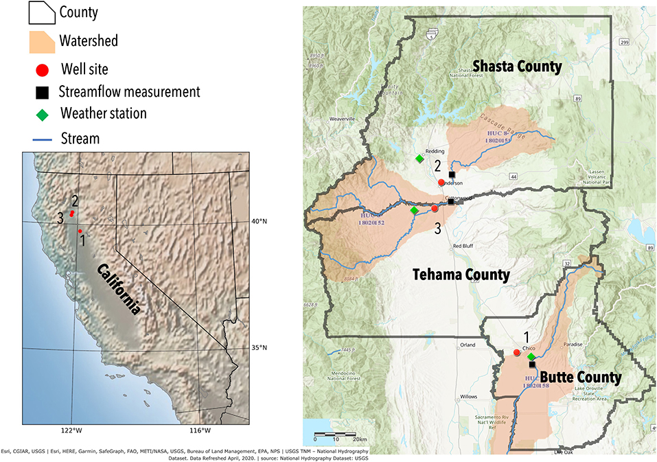
Figure 1. Location of the three well sites in California: Butte, Shasta, and Tehama County. The red dots show the location of the observation wells. Weather station (green diamond) and river flow monitoring station (black square) are located close to the well site. The map was created using ArcGIS® software by Esri.
The Butte County Well Site
The majority of Butte county is located in the Sacramento Valley groundwater basin which is filled with sediments from marine and terrestrial environments. The groundwater well in this study (22N01E28J001M) is a dedicated monitoring well of depth 200 m and screened at 140–170 m. The well site is located in the Vina subbasin of Butte county, which covers 750 sq. km of the northern portion of Butte county. This subbasin is categorized as a high priority basin under the 2019 SGMA basin prioritization report (DWR, 2020), showing an immediate need to mitigate the groundwater depletion therein. The aquifer system includes stream channel and alluvial fan deposits, and deposits of the Modesto and Tuscan formations (DWR, 2004). Groundwater is a major water source for about 150 sq. km of irrigated land in the basin. Out of the total county wide freshwater withdrawal, about 94% is attributed to groundwater pumping for different uses (Dieter et al., 2018) while the rest is from surface water withdrawals. The nearest discharge monitoring station (Butte Creek Durham) measures the daily discharge rate at the Butte Creek which is about 8 km from the well. The Butte Creek and the much larger Feather Creek are the main sources for surface water diversion in the county (Butte County Department of Water and Resource Conservation, 2016). Temperature and precipitation data were obtained from the Chico weather station located 7 km from the well.
The Shasta County Well Site
The groundwater well in Shasta County is an observation well (30N04W10H005M) of depth 49 m and screened at 33–48 m. It is located in the Anderson subbasin which is a part of the Redding Groundwater Basin covering an area of about 400 sq. km. This subbasin is one of the primary agricultural regions in the county, is categorized as a medium priority basin according to the SGMA guidelines (DWR, 2020). Eighty to ninety percent of the basin's precipitation typically occurs from November to April. The aquifer system is comprised of continental deposits of late Tertiary to Quaternary age. The Quaternary deposits include Holocene alluvium and Pleistocene Modesto and Riverbank formations (California Department of Water Resources, 2004). The nature of surface water-groundwater interaction across the basin is complex, both spatially and temporally, but in most areas shallow groundwater levels lead to groundwater discharge to surface streams. During pronounced drought conditions, groundwater levels may decline to a level such that streams that formerly gained river flow from groundwater discharge now recharge the groundwater system through streambed infiltration. Major water supplies in this region are provided by surface storage reservoirs (Bureau of Reclamation, 2011). Agricultural, industrial, and municipal groundwater users in the basin pump primarily from deeper continental deposits, whereas domestic groundwater users generally pump from shallower deposits. Groundwater withdrawals contribute about 54% of the total county wide freshwater withdrawal from different sources (Dieter et al., 2018). Although this well is closest to the Sacramento River, the nearest discharge monitoring station is located in Cow Creek, which feeds into the Sacramento River and is about 5 km away. Since the nearest discharge station in the Sacramento River was located 20 km upstream, we chose to use the discharge observations from the Cow Creek station, as the closest approximation of discharge trends and seasonality that determines surface water influence on groundwater behavior. The temperature and precipitation data were obtained from the Redding Fire station located 15 km from the well.
The Tehama County Well Site
The groundwater well in Tehama County is an observation well (29N04W20A002M) of depth 137 m, with a screen at 109–131 m depth. It is located in the Bowman subbasin which is categorized as a low priority basin. This subbasin, is also a part of the Redding groundwater basin covering 495 sq. km in the north central portion of the county. The aquifer system of the Bowman subbasin is comprised of continental deposits of late Tertiary to Quaternary age. The Quaternary deposits include Holocene alluvium (thickness ranging from 0 to 10 m) and Pleistocene Modesto and Riverbank Formations (thickness ranging from 0 to 15 m). The Tertiary deposits include the Pliocene Tehama Formation (thickness may reach up to 150 m) and Tuscan Formations (thickness may reach up to 750 m) (Ayres and Brown, 2008). The Bowman subbasin is primarily a rural area where groundwater is used for agriculture, domestic, and municipal purposes. Groundwater sources represent the majority of supply, followed by local surface water. During an average water year, Tehama County does not experience any water shortages since the water supply is generally higher than the water demand. Groundwater contributes about 37% of the county's total freshwater withdrawal (Dieter et al., 2018). The observation well is located 0.6 km from the Cottonwood Creek. However, the closest river flow monitoring station is located about 8 km from the test site. The weather data was obtained from the Davis Ranch station located 10 km from the well.
Input Features, Data Sources, and Preprocessing Methodology
For our DL model, we identified features that we expect to directly or indirectly impact groundwater levels including temperature (T), precipitation (P), and river flow (i.e., discharge; Q). Daily historical observations of these variables from 2010 to 2018 are used together with groundwater level measurements (G) to train the neural network models (Table 1). In addition, we use the week of the year of the measurements' timestamps as a training feature, which naturally represents the inherent seasonality in the dataset.
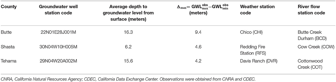
Table 1. Data sources of historical observations.
The observation wells indicate regional drawdowns due to groundwater extraction through pumping activities (for agriculture, urban use, or other). However, pumping data are not reported in California, and are not publicly available. Higher pumping rates are observed during summer months when the temperature is high with infrequent and small precipitation events and low surface water availability. Low precipitation years therefore lead to higher depletion rates, whereas wet years show lower depletion rates (Figure 2). Our assumption is that the ML model can capture the interaction between groundwater level and pumping through other proxy hydrological or climate variables that typically drive pumping (precipitation, temperature, or river flow).
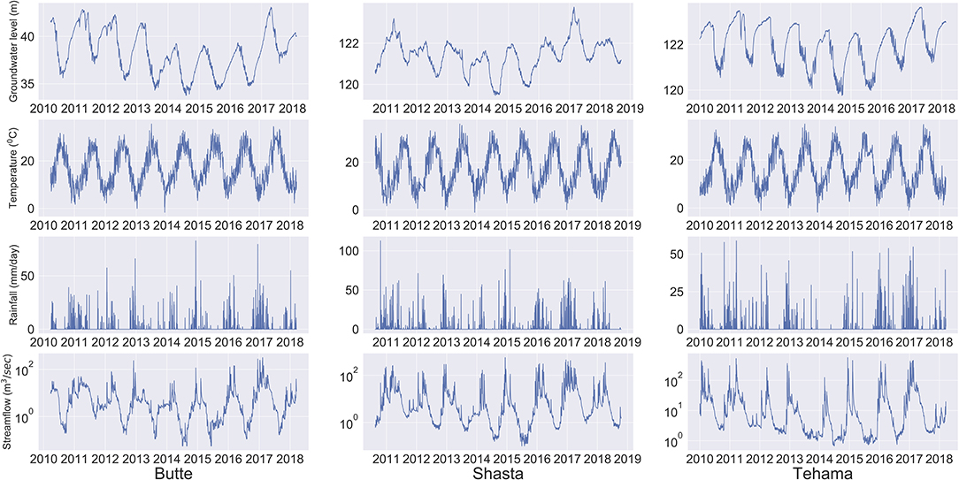
Figure 2. Timeseries of all features at the three well sites at a daily frequency from 2010 to 2018. The top panel at each site shows the groundwater level (meters above mean sea level). The second panel shows the temperature (°C), the third panel shows the precipitation (mm), and the bottom panel of sites shows the river flow (m3/sec).
All the datasets are processed for quality assurance and quality control (QA/QC), including gap-filling (also called as “missing value imputation”) and normalization. The QA/QC helps to remove erroneous values or outliers (unrealistic values) in the measurements due to faulty sensors or equipment failures, and the data gaps are then filled by using time series imputation techniques. We imputed the missing values using the imputeTS package (Moritz and Bartz-Beielstein, 2017) in R. This package is used for univariate time series imputation. We use the na.seadec (Seasonally Decomposed Missing Value Imputation) function with the application of the “kalman” algorithm, of the imputeTS package, which is well-suited for gap filling of time series exhibiting seasonality. Using this approach, the seasonal component is first removed, missing data are imputed in the general trend and then the seasonal component and the general trend are combined to generate a gap-filled uninterrupted time series. The missing values of each of the features in the datasets contribute to at most 2% of total length of the time series. The ratios of missing data to the total period at each monitoring station are provided in Supplementary Table 1.
Since our input features have significantly different ranges of absolute values, we scale each dataset to the range [0, 1]. This ensures that during the learning process (iterative weight adjustment) a percentage change in the weighted input sample is reflected with a similar percentage change at the nodes of the output layer (Kanellopoulos and Wilkinson, 1997). To this end, we use the minimum and the maximum values of each dataset. For temperature, precipitation, and river flow data, these lower, and upper limits are known and the task is unambiguous. Since the observed values for the river discharge have a huge variation (orders of magnitudes difference between summer and winter due to the lack of precipitation in California in the summer months), we log-normalized the values to attenuate the effect of high values that would occur in a uniform scaling. For the groundwater levels, determining the minimum and maximum levels is more difficult as the water table depths reached unprecedented lows during the 2012−2016 drought. Fixing the lower bound at the historically observed minimum value is unreliable, because future droughts may cause the lowest observed groundwater level to further decrease. A similar argument can be made for the maximum groundwater levels, which are expected to increase in particular for heavily overdrafted basins as sustainable groundwater management practices are being implemented. Thus, in this study, we set the minimum groundwater level to the lowest historically observed value less 15% and the maximum level to the highest historically observed value plus 15%. Given these lower and upper bounds, we then scale the groundwater data to [0, 1]. Note that scaling the input data values does not force the predicted values to remain within the lower and upper limits used for scaling.
Neural Network Model and Hyperparameter Tuning
In this study we implement an MLP type of neural network to build the groundwater prediction model. The MLP is a feedforward type of neural network with different hyperparameters that need to be adjusted before its training. The MLP was chosen as it was the best performing model in terms of accuracy and compute time, based on comparison with CNN, RNN, LSTM neural networks (Müller et al., 2020).
The choice of hyperparameters reflect the complexity of the MLP model. Hand tuning, grid and random sampling are the most widely used methods for choosing the hyperparameters of DL models (Bergstra and Bengio, 2012). Hand tuning is time consuming, it does not scale well to large search spaces, and it does not usually lead to the optimal hyperparameters. Thus, we use an automated hyperparameter optimization (HPO) method to find the best DL model hyperparameters.
We follow (Müller et al., 2020) to formulate a bilevel optimization problem:
where θ are the hyperparameters in the search space Ω; w are the weights and biases associated with each node in the MLP, and are the training and validation datasets, respectively. The search space Ω is a product of finite sets of integer values. At the upper-level optimization problem (Equation 1), the optimizer selects a set of hyperparameters θ (the model architecture). Given θ, the lower-level problem (Equation 3) is solved with RMSprop, in which we find optimal weights w* that minimize the loss function L for the training data. Once we obtain w*, we can then evaluate the upper-level objective function l that reflects how good a choice θ is. Based on the outcome for l, the optimizer at the upper-level selects the next set of hyperparameters for which the lower-level problem is solved, and so on until convergence at the upper-level is achieved. For solving the upper-level optimization problem, we use a derivative-free optimization algorithm that uses radial basis function surrogate models, see Müller et al. (2020) for further details. Since a stochastic optimizer is used to solve the lower-level problem (Equation 3), the performance of the MLP for a given architecture θ depends on the random number seed of the stochastic optimizer. Therefore, in order to obtain an approximated expected performance for a given MLP architecture, we solve the lower-level problem five times and average the results.
In our study, we search for the hyperparameters in a 6-dimensional search space, :
• Number of layers: θ1 ∈ { 1, 2, …, 6 }
• Number of nodes per layer: θ2 ∈ { 5, 10, …, 50 }
• Number of lags: θ3 ∈ { 30, 35, …, 365 }
• Dropout rate: θ4 ∈ { 0.1, 0.2, …, 0.5 }
• Batch size: θ5 ∈ { 50, 55, …, 200 }
• Epochs: θ6 ∈ { 50, 100, …, 500 }
and we map these numbers to consecutive integers for optimization. Thus, if we used complete enumeration to find the optimal MLP architecture, we would have to train 6, 120, 000 different MLPs, which is impractical for real-world decision-support applications. In the “upper level optimization,” we iteratively test only 50 different MLP neural network hyperparameters (50 different hyperparameter sets that describe the network architecture). This was sufficient to achieve convergence at the test site (Müller et al., 2020). To handle the lagged temporal relationship between variables, we use the concept of Time-Delayed Neural Network (Waibel et al., 1989). A consecutive set of observations is used as one input instead of one observation. We call this amount of historical data the lag. Lag is one of the most important hyperparameters in a feedforward neural network for handling time series data (Zhang, 2003).
We divide the observations of all the features into training (), cross-validation, (, finding the optimal hyperparameters), and testing data (), with a 50–25–25% split, except when indicated otherwise. The MLP models are trained to predict the groundwater level for the next time step (e.g., day or month). This output is computed based on the values of all features at the current time step and several previous time steps (equal to the lag number). For example, with a lag of 4-time steps, measurements of all features including the groundwater level from the past 4-time steps are used along with the current time step's data, to predict the groundwater level at the next time step. The MLP's output is a single groundwater level value for the next time step. When training the MLP for a given set of hyperparameters, observed values of all features are used to optimize the weights in the MLP model. During cross-validation and testing, the observed values of only temperature, precipitation, river flow, and week of year are used as drivers for making groundwater level predictions. To make groundwater level predictions over several time steps, the predicted groundwater level from the previous timestep is recursively incorporated with the observed values of temperature, precipitation and river flow to make the new input sample. Using the recursive approach during the testing and validation period, we test the capability of the MLP model to make multi-month predictions of groundwater level using projections of future meteorological or hydrological features. This can potentially enable decision support for sustainable groundwater management in the long run.
In this study, we use backpropagation (Rumelhart et al., 1986) to train the MLP. Hyperparameters such as activation functions and the optimization method used in training the MLP are fixed (Rectified linear unit (Nair and Hinton, 2010) and RMSprop (Tieleman and Hinton, 2012), respectively). We conducted our numerical experiments with python (version 3.7) on Ubuntu 16.04 with Intel® Xeon(R) CPU E3-1245 v6 @ 3.70GHz ×8, and 31.2 GiB memory. We use the Keras package (Chollet, 2016) with the TensorFlow (Abadi et al., 2016) backend for our deep learning architectures.
DL Model Ensembles to Quantify Prediction Accuracy and Variability
Given that a DL model training involves a stochastic optimizer, we cannot infer prediction accuracy from a single DL model trial. Thus, we train the model multiple times (Ne = 20 trials) for the same DL model architecture and the same inputs to gain insights into the inherent prediction variability. Each trial generates a future groundwater level prediction of Nt time steps and a corresponding error between the predicted and the observed values for all time steps of the testing period. The accuracy of a trial i is quantified by the RMSE (δi) of the groundwater prediction (Gpred), which is computed in Equation (4). The average of the error (δi) generated across the trials gives the mean prediction error (δ) of the MLP model (Equation 5).
where is the groundwater prediction made at the jth time step for the ith trial, is the corresponding observed groundwater level at the jth timestep. The testing period of Nt time steps starts from time step k in the dataset and runs until Nt + k − 1 time step. In order to quantify the prediction variability, at each time step j, we compute the standard deviation (σj) of the ensemble over the Ne trials (Equation 6). We compute the standard deviation as follows:
To compute the overall prediction variability (S) of a DL model architecture, the average of the standard deviations σj; j = k, …, k + Nt − 1 is computed as indicated in Equation (7). Lower values of S means the DL model architecture is more robust to the stochasticity in the training.
Sensitivity Analysis of DL Model Predictions
In our numerical study we examine how different combinations of input features and the length of training time series affect the prediction accuracy of the DL model. These combinations represent potential settings in different watersheds where different amounts and types of data are collected by local agencies. This study enables us to identify input data that are necessary and sufficient for making accurate predictions of future groundwater levels. It also allows us to gain insights into “how much accuracy we lose” when certain data are not available. We examine eight different input feature scenarios for training the MLP model (Table 2). For example, the experiment labeled G-T-P-4-d indicates that groundwater, temperature, precipitation, and week of year are used as input features. The number 4 indicates that we used 4 years of historical observations as training data and d indicates a daily data resolution for validation and testing. Using data at the monthly resolution (indicated by m) means that the number of training data points is reduced by 97%. In this scenario, we also replace the week of year feature with the month of the year.
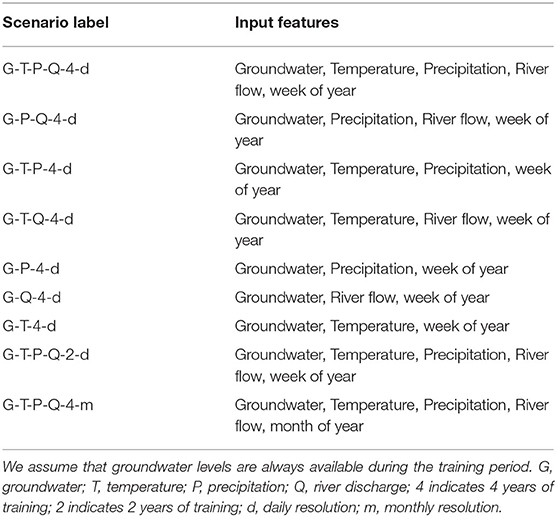
Table 2. Combinations of input features for training the DL model.
We designed the numerical experiments such that they address the following questions: (1) Which input features are sufficient to predict the groundwater level accurately? (2) Is there a minimum amount of data necessary to build a reasonably accurate prediction model? (3) How robust are the DL model predictions given different input feature combinations?
In order to answer these questions, we optimized and trained the MLP for each experiment shown in Table 2. We cannot expect the same DL model to perform well for all experiments, because the lack of certain input features potentially requires different model architecture, and if not adjusted, using too complex models may lead to data overfitting. For each experiment, we solve the bi-level optimization approach described in the section Neural Network Model and Hyperparameter Tuning to find the best model architecture. We solve the lower level problem five times to obtain an average model performance. For the optimal hyperparameter choice, we train the MLP network Ne = 20 times, each time generating a different MLP model. Using the resulting model ensemble, we obtain Ne replications of future groundwater predictions, which allow us to compute the statistics of the DL model performance, to quantify the prediction variability, and analyze the sensitivity of the model predictions to the input data.
Numerical Results
In this section we describe the results of our numerical experiments and provide a discussion of their implications on our guiding questions.
Sensitivity Analysis of Prediction Errors
We compare the future predictions obtained with our optimized and trained MLPs when using the different input feature scenarios described in Table 2. We make predictions for a time frame that was not used during optimization or training of the MLP (2 years unless otherwise specified), to assess the ability of the models to extrapolate beyond their training time frame.
We find that for all sites the mean prediction error ( δ ) ranges from 0.4 to 3.7 m (Table 3). Ideally, a good predictive model has low prediction errors and low variability. From the numerical results, we observe that for the Butte well, we achieve the lowest mean prediction error when training the model on G-P-4-d scenario and the lowest prediction variability in the G-T-P-Q-4-d scenario. For both Shasta and Tehama wells, we find multiple scenarios that give the same lowest values of prediction error and prediction variability.
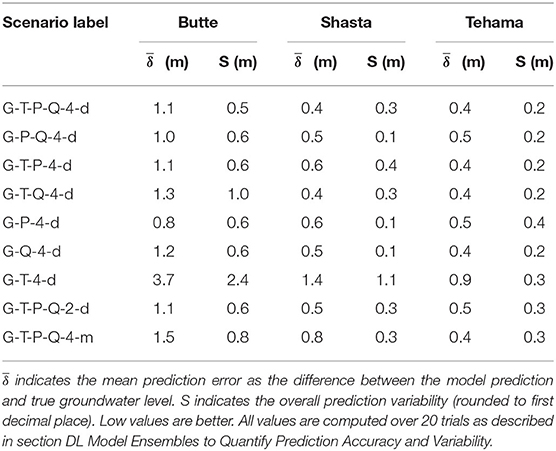
Table 3. MLP predictive performance at all three sites and for nine scenarios.
The MLP model that is optimized and trained on all input features (Groundwater, Temperature, Precipitation and River flow) performs reasonably well across all the locations, showing similar values of normalized error of about 0.1 or 10% of Δmax (Figure 3), where Δmax is the difference between the observed maximum and minimum groundwater levels. We use this scenario (G-T-P-Q-4-d) as the base scenario in the following per-site analysis to understand the sensitivity of different input features.
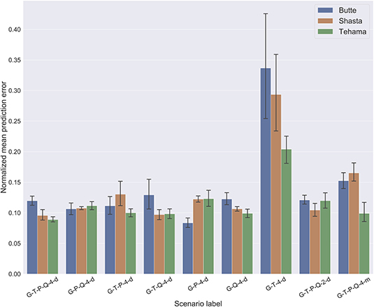
Figure 3. Barplot comparing the normalized mean prediction error and their standard deviation at all well-sites for all experiments. The normalized values are obtained by dividing the error by the difference between the maximum and minimum observed groundwater levels (Δmax). This normalization helps us to compare model performance across different locations. Lower bars indicate smaller prediction errors and therefore better model performance. The errors were computed by comparing the true and predicted groundwater levels in the testing dataset.
Butte Site
The Butte site is highly sensitive to the precipitation data (the prediction error increases significantly compared to the base case scenario when we remove precipitation as an input feature). In fact, the MLP model trained only on groundwater and precipitation provides the lowest prediction error. A comparison of the prediction errors of the G-P-Q-4-d and G-Q-4-d scenarios with the base scenario reveals that the precipitation events in the past are most likely to impact the future groundwater availability at this site. As the groundwater table at this site is fairly deep (16 m below ground surface), we postulate that river flow likely does not directly impact the groundwater level at the well site. Instead, given the high proportion of water use being groundwater at this site, the water table are likely driven by pumping and dependent on the amount of rainfall received over the past year.
Shasta Site
Based on simulations with different input feature scenarios, we observe that the Shasta site is most sensitive to the river flow feature. This can be seen by the error differences between the scenarios G-T-P-Q-4-d and G-T-P-4-d. Precipitation is the second most important feature. Although the river flow feature is generated using Cow Creek discharge rates, given our scaling and normalization procedure, we assume it is representative of the discharge fluctuations in the Sacramento River (which is closer to the well site). The sensitivity to river flow can be attributed to the shallow depth to groundwater (about 6 m), and short distance from the river, suggesting possible hydraulic connectivity.
Tehama Site
The MLP model trained on the base case scenario gives the lowest prediction error. We observe relatively small changes in prediction accuracy when input features such as river flow and precipitation are individually removed, showing equal input feature sensitivity. The MLP model trained only on groundwater and river flow (G-Q-4-d) also gives the same prediction performance as the base scenario. However, this is not observed when the MLP model is trained only on groundwater and precipitation (G-P-4-d), or groundwater and temperature (G-T-4-d). This indicates that the river flow carries more groundwater-relevant information, followed by precipitation in this region. This is consistent with the relatively low reliance on groundwater for water use in this region.
In all cases, the predictions are the worst when all input features except for groundwater and temperature are removed. In the following sections we only present summarized findings from the numerical experiments. The groundwater level prediction results of the individual scenarios at each of the test sites are provided in Supplementary Section 3.
Stochasticity in Training and Associated Prediction Variability
In order to better illustrate the stochasticity associated with the training process, we train an MLP with the same architecture but with different random number seeds. This results in a slightly different model for each run. For example, three different trials resulted in three different accuracies, with some trials yielding much more accurate outcomes than others (Figure 4). Therefore, we should not base decisions for groundwater management on a single trial with an MLP.
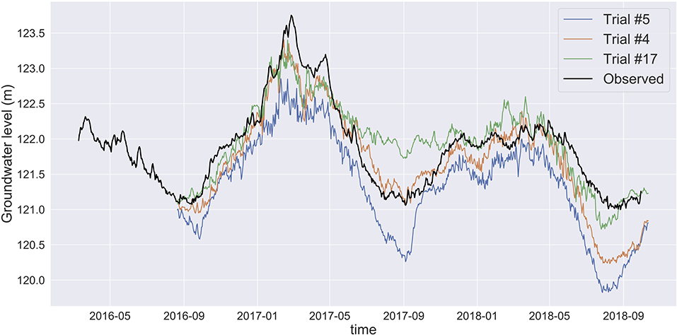
Figure 4. MLP prediction for three trials with the same input features and hyperparameters at Shasta with different random seeds. The black time series shows the observed groundwater level and the other colors represent predictions from three ensemble members. The stochasticity in the training leads to different MLP models and corresponding different predictions. The prediction indicated by the Trial #5 (blue line) shows a large decrease of the groundwater level and has the highest prediction error. Trial #4 (orange line) is closest to the observed groundwater levels (truth) while Trial #17 (green line) shows a more optimistic future with less groundwater depletion.
At the Butte well site the prediction variability (S) resulting from the stochasticity in training shows the highest sensitivity to the precipitation feature followed by the river flow feature (Figure 5). By comparing the different scenarios across all well sites, we find that the MLP models trained on groundwater and temperature features (G-T-4-d) have a wider spread in the predictions.
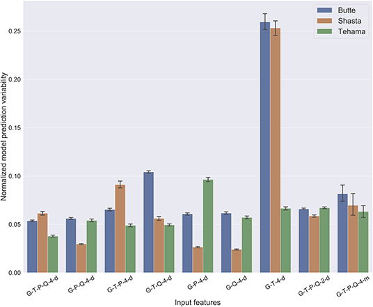
Figure 5. Barplot comparing normalized model prediction variability (S). Lower S values indicate more robust MLP models that make more reliable predictions, while higher values indicate a higher variability in future predictions. The model prediction variability S is also normalized in the same way as the mean prediction error . The standard deviation of S, represented by the black line on each bar indicates the variation in the ensemble prediction spread across all time steps.
We illustrate the increasing variability of the MLP predictions when excluding necessary input features in Figures 6, 7. The prediction ensemble generated with all input features (G-T-P-Q-4-d) at the Butte site is able to predict the groundwater levels over the 2 years with good accuracy (Figure 6). On the other hand, the predictions at Butte site when using only groundwater and temperature data for training the MLP have low prediction accuracy and high prediction variability (Figure 7). Although the model is still able to capture the seasonality of the groundwater levels, the differences between the observed and the mean of the predicted groundwater levels are large. We conducted a similar analysis for Shasta and Tehama (see Supplementary Sections 3.1 and 3.7). Note, however, that low prediction variability does not automatically imply high prediction accuracy, and thus both variability and prediction accuracy must be considered.
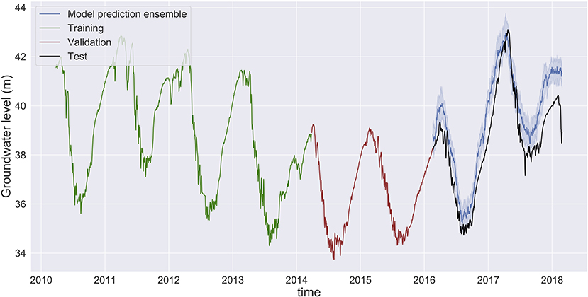
Figure 6. Groundwater level prediction at Butte with input features: groundwater level, temperature, precipitation, and river flow (G-T-P-Q-4-d). The small differences between the predicted groundwater levels (ensemble mean, dark blue) and the observed levels (black) indicate a high prediction accuracy. The narrow blue band around the mean prediction indicates higher reliability in model prediction, and thus low prediction variability. Predictions made by MLP models in Shasta and Tehama are provided in Supplementary Figures 1, 2.
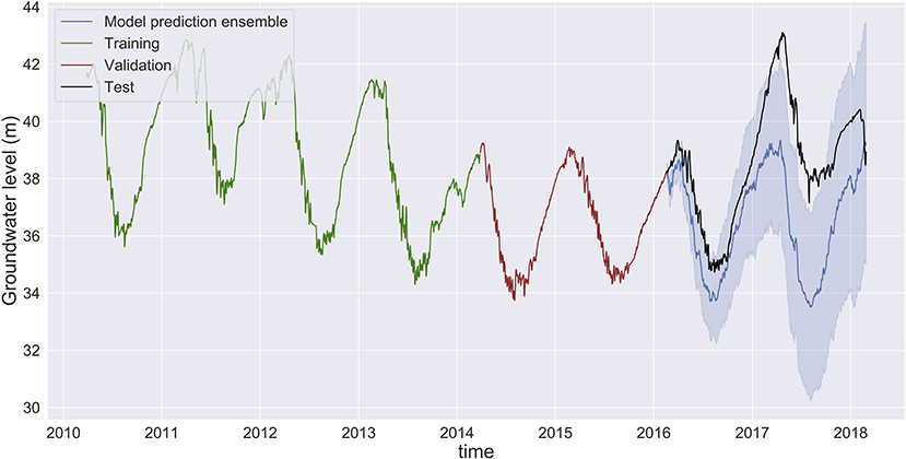
Figure 7. Groundwater level prediction at Butte with input features: groundwater and temperature. Large differences between the ensemble mean (dark blue) and observed (black) show low prediction accuracy. The high variability of the predictions of individual ensemble members (blue band) shows that the MLP model is not reliable. Predictions made by MLP models in Shasta and Tehama are provided in Supplementary Figures 18, 19.
Analysis of Monthly vs. Daily Training Data
Climate model data and groundwater observations are often available at a monthly temporal resolution rather than at a daily frequency. Therefore, we examined the effect of using lower-resolution data for training the MLP model, by averaging the daily values for each month. Using monthly data means that, for the same date range, the number of available training points is significantly lower: the total amount of data points is reduced by about 97% (≈100 monthly vs. ≈2, 900 daily). The groundwater predictions at Butte trained on monthly data are much smoother and the daily groundwater drawdowns (high frequency oscillations that we observe in the daily data) are not present (Figure 8). The predictions show that the MLP is still able to capture the seasonality in the data (lower groundwater levels in the summer, higher levels in the winter). When compared to the corresponding daily frequency model at Butte, G-T-P-Q-4-d (Figure 6), we observe that the prediction errors are higher and the model does not pick up on the larger amounts of water that are available during the wet years (2017 and 2018). The prediction variability is also relatively low, indicating that for monthly predictions, the stochasticity that arises from training the models is lower, perhaps due to overfitting. At Shasta, the MLP model trained on monthly data shows a lower prediction accuracy and higher prediction variability than the base scenario. At Tehama, the MLP model built on monthly data shows similar prediction accuracy, but a higher prediction variability in comparison to the daily frequency base scenario suggesting a lack of sufficient training data to build a robust model (see Supplementary Figure 24).
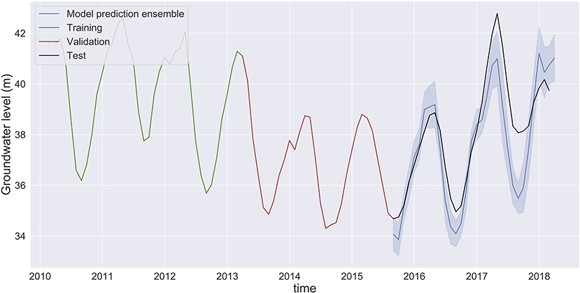
Figure 8. Groundwater level prediction at Butte using monthly averaged data for all features (groundwater, temperature, precipitation, and river flow). Although the ensemble spread is narrow (the model predictions are reliable), the prediction error is high, indicating a lack of sufficiently numerous training data points.
Choice of Optimal Lag Hyperparameter
The lag hyperparameter helps the MLP model capture long-term dependencies between groundwater and other features. As mentioned previously the input to the MLP model is a lagged time series data at each timestep (section Neural Network Model and Hyperparameter Tuning). A lag number of 30 indicates that 30 days of past observations of the features are required to make the next-day groundwater level prediction. The lag parameter is a hyperparameter that is automatically optimized. Table 4 lists the optimal lags that lead to the best groundwater level predictions. At the Butte site, we observe that most input feature combinations require a lag > 300 days. When using monthly data, the optimal lag is 23 months (≈2 years). At Shasta, the optimal lag values are > 70 days; at Tehama, the optimal lag values are > 260 days. The results indicate that the optimal lag is dependent on the specific experimental conditions and cannot be generalized to be the same across different scenarios and well sites. An incorrect lag can be detrimental to the model's predictive performance. Values of the other hyperparameters chosen are presented in Supplementary Tables 2–4.
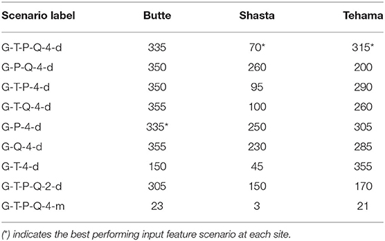
Table 4. Optimal lag hyperparameter chosen in the hyperparameter optimization process at all three sites and for each scenario.
Sensitivity Analysis of the Prediction Performance to the Length of the Training Time series Data
Analyzing the sensitivity of the MLP's predictive performance to the length of the training data addresses two questions. First, we will examine if the predictive performance of the MLP model is reduced by using a smaller training set. Second, by using a shorter time series for HPO and training, we can assess the accuracy of groundwater predictions for a longer time period. We experiment with using only 2 years of data for training and 2 years of validation, thus testing the MLP's prediction accuracy over 4 years. At the three sites, our MLP models are still able to predict the groundwater levels fairly accurately compared to the base scenario (Figure 3).
At the Butte site, the overall prediction accuracy is the same as the base scenario with a slightly higher prediction variability (Figure 9). The seasonality in the groundwater levels (less water in the summer and more in the winter) is captured well. The groundwater predictions are close to the true values for the first 1.5 years of prediction (2014–2015), but in the subsequent years the model predictions fail to accurately capture the highs and lows. The errors of the groundwater predictions accumulate over time, due to how we make next-day predictions [use the previous [lag] days of groundwater level data, and at some point, we start making predictions based on predictions and thus the errors accumulate]. At the Tehama site (see Supplementary Figure 22), the MLP model makes accurate predictions for the first 2 years (2014 and 2015) and subsequently we observe that the MLP predictions fail to capture the highs and the lows. This may either be related to error accumulation or a missing feature, such as snow pack or pumping data. A similar result holds for the Shasta well: the MLP is able to capture the seasonal behavior of the groundwater levels, but as we make predictions over multiple years, the prediction inaccuracies increase (see Supplementary Figure 21).
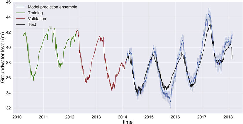
Figure 9. Groundwater level prediction at Butte with input features: groundwater level, temperature, precipitation, and river flow when using only 2 years of data each for hyperparameter optimization process and training. The MLP is able to capture the seasonality of the groundwater levels, and it reflects well the groundwater levels during the drought years and the wet years.
Discussion
Future Prediction Using MLP Models
With a suitable choice of input features (e.g., G, T, P, and Q), MLP models can reliably predict groundwater levels for up to 1 year and possibly longer at a daily frequency. This is observed at all sites despite the differences in the contribution of groundwater to the county's water budget. In addition, models built exclusively with meteorological variables using temperature, precipitation and groundwater as input features (G-T-P-4-d) also show a good prediction accuracy of about 85–90%. Long-term forecasts of these meteorological variables generated from different weather models can potentially be used to predict future groundwater levels. This can help derive sustainable groundwater management strategies.
Impact of Data Availability
A major challenge in this study was the selection of well sites and monitoring stations that adequate measurement for training, and located in near proximity. For example, at the Shasta site, we would ideally use the discharge rate of the Sacramento River rather than the Cow Creek in the MLP model. But we did not find such a monitoring station near the well site. On the other hand, it is also difficult to find groundwater wells with a long period of measurements close to river flow or weather monitoring stations. Experiments with MLP models trained on monthly averaged data and the analysis of optimal lag hyperparameter chosen at the three sites (for different scenarios) also suggest that access to a longer time range of data can help build better prediction models. This recurring issue of site selection currently makes DL techniques inapplicable in the majority of watersheds in California.
Models built from monthly frequency data show a higher prediction error than the daily frequency-based model and are unreliable for making long term (multi-year) predictions. We found that daily data were unavailable for most of the sites in California. In fact, out of the 3,907 monitoring wells in the state, only 387 had daily measurements through California statewide groundwater elevation monitoring (CASGEM) network, and most of the high-resolution datasets were only available for wells in northern California, in mostly low-priority basins. Prediction accuracies can be improved with access to higher-resolution daily data, or longer monthly datasets (spanning decades). Additionally, our current analysis is performed in the absence of pumping data, which is not publicly available. Yet pumping is a critical component of groundwater budget, and in several places the primary driver of groundwater table depths. Access to such data can potentially better equip our current DL models with human behavior and improve management strategies. The potential advantage of using additional data for obtaining more accurate predictions may lead to investments into more in-situ or remote measurement infrastructure. Based on our current results, we recommend using more than 2 years of daily data for training.
Impact of Training Stochasticity on Prediction Results Matters
In addition to the prediction accuracy, we find that it is also important to measure the prediction variability of the MLP, which is due to stochasticity in the training process. The Keras tool used in the study generated different weight optimized MLP models for the same set of hyperparameters and training data. We cannot analyze future predictions or derive water management strategies based on a single training trial. We recommend training a DL model of a given architecture multiple times, as the stochasticity of the optimizer used during the training leads to multiple prediction models that are consistent with the training data. The resulting model ensembles allow us to assess the model's prediction reliability. Thus, in addition to potential uncertainty in the data collected we also need to take into account the variability in the training process. Our study showed that models trained on groundwater, temperature, precipitation, and temperature data (G-T-P-Q-4-d) yield the lowest prediction variability, whereas models trained only on groundwater and temperature data have the highest prediction variability. Note however, that low variability does not necessarily mean high prediction accuracy, and thus both metrics need to be taken into account when assessing the quality of the DL model predictions. In a future study, one can tackle this problem from a bi-objective perspective in which the prediction accuracy is maximized and the variability is minimized simultaneously.
Automated HPO Framework for Future DL Applications
A key innovation in this study is the use of an HPO framework to test different model architecture for making prediction models. The setup of our study, and the HPO is general enough to be applicable to any other type of neural network (e.g., CNN and LSTM). The sensitivity analysis requires conducting multiple experiments testing different input feature combinations and our results indicate that each experiment requires a different combination of hyperparameters. Hand tuning the model architectures for each experiment can be a cumbersome process especially when the number of features is large. The HPO framework used in this study automates this process and ensures the best model architecture (within the given bounds). We can also potentially incorporate the choice of input feature into the framework as a decision variable. The HPO formulation will then choose the best combination of input features and its best architecture simultaneously.
Multi-Well MLP Models
The current analysis has been conducted for single groundwater well sites only, which does not reflect the overall health of a groundwater aquifer. Thus, a spatially distributed parameter sensitivity analysis across multiple groundwater well sites and climatic parameters may reflect a more realistic behavior of a groundwater aquifer and human use. Our previous study (Müller et al., 2020) successfully built DL models to simultaneously predict daily groundwater level at three locations in Butte county. However, we saw that when we use an average prediction error metric to measure the prediction performance across the three wells, only two wells have accurate predictions. Thus, one remedy could be a reformulation of the objective function by introducing weights that reflect the importance of each well to ensure optimal prediction performance across all wells. Although training can be compute-intensive, once trained and optimized, DL models are a more viable option for performing multi-scenario analyses than high-fidelity simulation models, because the required computational time to make future predictions is orders of magnitude lower. Our multi-scenario analysis can readily be used by groundwater managers who have access to historical groundwater and local weather data.
Conclusion
With the increased deployment of ML tools in hydrological sciences, there is a need to understand the sensitivity of their prediction performance to different input features. Groundwater level timeseries are highly non-linear and non-stationary, making them difficult to model with standard ARIMA models. DL models offer a promising alternative for capturing the complex interactions between features such as groundwater levels, river flow, temperature, and precipitation.
In our study, we were able to accurately predict groundwater levels at three different groundwater well locations (Butte, Shasta, and Tehama) in California using an MLP model. Additionally, we conducted a sensitivity analysis using multiple different feature combination scenarios and compared the accuracy and reliability of the resulting predictions. Our analysis shows that models trained on groundwater, temperature, river flow and precipitation data (G-T-P-Q-4-d) lead to the best predictive performance at two of the three sites, while models trained without hydrological features and based only on past groundwater and temperature data consistently showed the lowest prediction accuracy at all locations. The best predictive models are shown to reliably predict groundwater levels at least 1 year into the future. The MLP prediction performance is also affected by the data's temporal resolution and the length of the training period. The MLP models trained with only 2 years (rather than four) of data still gave reasonable accuracy and indicate the potential capability for long-term predictions. In addition to accuracy, we find that it is also important to measure the prediction variability caused by the stochasticity in the training process. The MLP model architectures for different choices of input features, training length and temporal frequency which were obtained using a hyperparameter optimization framework indicate that the optimal combination is location-specific. These results indicate that DL models are a good choice for modeling groundwater levels, contingent on the availability of adequately long time-series of prior groundwater levels and some hydrological variables (precipitation or river flow at the minimum).
Data Availability Statement
The raw data supporting the conclusions of this article will be made available by the authors, without undue reservation.
Author Contributions
RS, JM, CV, BA, and BF conceived the presented idea. RS and JP carried out the numerical experiment. RS wrote the manuscript with support from other authors. All authors provided critical feedback and helped shape the research, analysis, and manuscript.
Funding
This work was supported by Laboratory Directed Research and Development (LDRD) funding from Berkeley Lab, provided by the Director, Office of Science, of the U.S. Department of Energy under Contract No. DE-AC02-05CH11231.
Conflict of Interest
The authors declare that the research was conducted in the absence of any commercial or financial relationships that could be construed as a potential conflict of interest.
Supplementary Material
The Supplementary Material for this article can be found online at: https://www.frontiersin.org/articles/10.3389/frwa.2020.573034/full#supplementary-material
References
Abadi, M., Agarwal, A., Barham, P., Brevdo, E., Chen, Z., Citro, C., et al. (2016). Tensorflow: Large-scale machine learning on heterogeneous distributed systems. arXiv [Preprint] arXiv:1603.04467.
Adamowski, J., and Chan, H. F. (2011). A wavelet neural network conjunction model for groundwater level forecasting. J. Hydrol. 407, 28–40. doi: 10.1016/j.jhydrol.2011.06.013
Adamowski, J., Fung Chan, H., Prasher, S. O., Ozga-Zielinski, B., and Sliusarieva, A. (2012). Comparison of multiple linear and nonlinear regression, autoregressive integrated moving average, artificial neural network, and wavelet artificial neural network methods for urban water demand forecasting in Montreal, Canada. Water Resour. Res. 48. doi: 10.1029/2010WR009945
Aeschbach-Hertig, W., and Gleeson, T. (2012). Regional strategies for the accelerating global problem of groundwater depletion. Nat. Geosci. 5, 853–861. doi: 10.1038/ngeo1617
Ahmad, S., Kalra, A., and Stephen, H. (2010). Estimating soil moisture using remote sensing data: a machine learning approach. Adv. Water Resour. 33, 69–80. doi: 10.1016/j.advwatres.2009.10.008
Amari, S. I. (1993). Backpropagation and stochastic gradient descent method. Neurocomputing 5, 185–196. doi: 10.1016/0925-2312(93)90006-O
Arora, B., Mohanty, B. P., and McGuire, J. T. (2011). Inverse estimation of parameters for multidomain flow models in soil columns with different macropore densities. Water Resour. Res. 47:2010WR009451. doi: 10.1029/2010WR009451
Arora, B., Mohanty, B. P., and McGuire, J. T. (2012). Uncertainty in dual permeability model parameters for structured soils. Water Resour. Res. 48:W01524. doi: 10.1029/2011WR010500
Ayres, J., and Brown, C. (2008). Tehama County AB-3030 Groundwater Management Plan. Retrieved from: http://www.tehamacountypublicworks.ca.gov/flood/groundwater/bowman.pdf (accessed April 20, 2020).
Banerjee, P., Singh, V. S., Chatttopadhyay, K., Chandra, P. C., and Singh, B. (2011). Artificial neural network model as a potential alternative for groundwater salinity forecasting. J. Hydrol. 398, 212–220. doi: 10.1016/j.jhydrol.2010.12.016
Bergstra, J., and Bengio, Y. (2012). Random search for hyper-parameter optimization. J. Machine Learn. Res. 13, 281–305. Available online at: https://dl.acm.org/doi/abs/10.5555/2188385.2188395
Bureau of Reclamation Mid Pacific Region Sacramento California US department of Interior Anderson-Cottonwood Irrigation District. (2011). Anderson-Cottonwood Irrigation DistrictIntegrated Regional Water Management Program – Groundwater Production Element Project. Available online at: https://www.waterboards.ca.gov/waterrights/water_issues/programs/bay_delta/california_waterfix/exhibits/docs/CSPA%20et%20al/aqua_60.pdf (accessed April 20, 2020).
Butte County Department of Water Resource Conservation. (2016). Butte County Water Inventory and Analysis. Available online at: https://www.buttecounty.net/wrcdocs/Reports/I%26A/2016WI%26AFINAL.pdf (accessed April 20, 2020).
California Department of Water Resources (2004). Anderson Subbasin Hydrogeology. Retrieved from: https://water.ca.gov/-/media/DWR-Website/Web-Pages/Programs/Groundwater-Management/Bulletin-118/Files/2003-Basin-Descriptions/5_006_03_AndersonSubbasin.pdf (accessed April 20, 2020).
Chollet, F. (2016). Keras Deep Learning Library. Code:Available online at: https://github.com/fchollet (accessed April 20, 2020). Documentation: http://keras.io (accessed April 20, 2020).
Deka, P. C. (2014). Support vector machine applications in the field of hydrology: a review. Appl. Soft Comput. 19, 372–386. doi: 10.1016/j.asoc.2014.02.002
Deo, R. C., and Sahin, M. (2016). An extreme learning machine model for the simulation of monthly mean streamflow water level in eastern Queensland. Environ. Monitor. Assess. 188:90. doi: 10.1007/s10661-016-5094-9
Dieter, C. A., Maupin, M. A., Caldwell, R. R., Harris, M. A., Ivahnenko, T. I., Lovelace, J. K., et al. (2018). Estimated Use of Water in the United State in 2015. Reston, VA: U.S. Geological Survey Circular. doi: 10.3133/cir1441
DWR California Department of Water Resources. (2004). Vina Subbasin Hydrogeology. Retrieved from: https://water.ca.gov/-/media/DWR-Website/Web-Pages/Programs/Groundwater-Management/Bulletin-118/Files/2003-Basin-Descriptions/5_021_57_VinaSubbasin.pdf (accessed April 20, 2020).
DWR California Department of Water Resources. (2020). Basin Prioritization. Retrieved from: https://water.ca.gov/Programs/Groundwater-Management/Basin-Prioritization (accessed April 20, 2020).
Emamgholizadeh, S., Moslemi, K., and Karami, G. (2014). Prediction the groundwater level of bastam plain (Iran) by artificial neural network (ANN) and adaptive neuro-fuzzy inference system (ANFIS). Water Resour. Manag. 28, 5433–5446. doi: 10.1007/s11269-014-0810-0
Gaur, S., Ch, S., Graillot, D., Chahar, B. R., and Kumar, D. N. (2013). Application of artificial neural networks and particle swarm optimization for the management of groundwater resources. Water Resour. Manag. 27, 927–941. doi: 10.1007/s11269-012-0226-7
Ghiassi, M., Zimbra, D. K., and Saidane, H. (2008). Urban water demand forecasting with a dynamic artificial neural network model. J. Water Resour. Plann. Manag. 134, 138–146. doi: 10.1061/(ASCE)0733-9496(2008)134:2(138)
Guzman, S. M., Paz, J. O., and Tagert, M. L. M. (2017). The use of NARX neural networks to forecast daily groundwater levels. Water Resour. Manag. 31, 1591–1603. doi: 10.1007/s11269-017-1598-5
Herrera, M., Torgo, L., Izquierdo, J., and Pérez-Garćia, R. (2010). Predictive models for forecasting hourly urban water demand. J. Hydrol. 387, 141–150. doi: 10.1016/j.jhydrol.2010.04.005
Kanellopoulos, I., and Wilkinson, G. G. (1997). Strategies and best practice for neural network image classification. Int. J. Remote Sens. 18, 711–725. doi: 10.1080/014311697218719
Kratzert, F., Klotz, D., Brenner, C., Schulz, K., and Herrnegger, M. (2018). Rainfall–runoff modelling using long short-term memory (LSTM) networks. Hydrol. Earth Syst. Sci. 22, 6005–6022. doi: 10.5194/hess-22-6005-2018
Langevin, C. D., Hughes, J. D., Banta, E. R., Niswonger, R. G., Panday, S., and Provost, A. M. (2017). Documentation for the MODFLOW 6 groundwater flow model. Reston, VA: U.S. Geological Survey. doi: 10.3133/tm6A55
Lin, J. Y., Cheng, C. T., and Chau, K. W. (2006). Using support vector machines for long-term discharge prediction. Hydrol. Sci. J. 51, 599–612. doi: 10.1623/hysj.51.4.599
Mohanty, S., Jha, M. K., Raul, S. K., Panda, R. K., and Sudheer, K. P. (2015). Using artificial neural network approach for simultaneous forecasting of weekly groundwater levels at multiple sites. Water Resour. Manag. 29, 5521–5532. doi: 10.1007/s11269-015-1132-6
Moosavi, V., Vafakhah, M., Shirmohammadi, B., and Behnia, N. (2013). A wavelet-ANFIS hybrid model for groundwater level forecasting for different prediction periods. Water Resour. Manag. 27, 1301–1321. doi: 10.1007/s11269-012-0239-2
Moritz, S., and Bartz-Beielstein, T. (2017). imputeTS: time series missing value imputation in R. R J. 9, 207–218. doi: 10.32614/RJ-2017-009
Müller, J., Park, J., Sahu, R., Varadharajan, C., Arora, B., Faybishenko, B., et al. (2020). Surrogate optimization of deep neural networks for groundwater predictions. J. Glob. Optim. doi: 10.1007/s10898-020-00912-0
Nair, V., and Hinton, G. E. (2010). “Rectified linear units improve restricted boltzmann machines,” in Proceedings of the 27th International Conference on Machine Learning (ICML-10), Haifa. 807–814.
Najah, A., El-Shafie, A., Karim, O. A., and El-Shafie, A. H. (2013). Application of artificial neural networks for water quality prediction. Neural. Comput. Appl. 22, 187–201. doi: 10.1007/s00521-012-0940-3
Rasouli, K., Hsieh, W. W., and Cannon, A. J. (2012). Daily streamflow forecasting by machine learning methods with weather and climate inputs. J. Hydrol. 10:198. doi: 10.1016/j.jhydrol.2011.10.039
Rode, M., Wade, A. J., Cohen, M. J., Hensley, R. T., Bowes, M. J., Kirchner, J. W., et al. (2016). Sensors in the stream: the high-frequency wave of the present. Environ. Sci. Technol. 50, 10297–10307. doi: 10.1021/acs.est.6b02155
Rumelhart, D. E., Hinton, G. E., and Williams, R. J. (1986). Learning representations by back-propagating errors. Nature 323, 533–536. doi: 10.1038/323533a0
Sahoo, S., Russo, T. A., Elliott, J., and Foster, I. (2017). Machine learning algorithms for modeling groundwater level changes in agricultural regions of the U.S. Water Resour. Res. 53, 3878–3895. doi: 10.1002/2016WR019933
Shen, C. (2018). A transdisciplinary review of deep learning research and its relevance for water resources scientists. Water Resour. Res. 54, 8558–8593. doi: 10.1029/2018WR022643
Siebert, S., Burke, J., Faures, J. M., Frenken, K., Hoogeveen, J., Döll, P., et al. (2010). Groundwater use for irrigation - A global inventory. Hydrol. Earth Syst. Sci. 14, 1863–1880. doi: 10.5194/hess-14-1863-2010
Steefel, C. I., Appelo, C. A. J., Arora, B., Jacques, D., Kalbacher, T., Kolditz, O., et al. (2015). Reactive transport codes for subsurface environmental simulation. Computat. Geosci. 19, 445–478. doi: 10.1007/s10596-014-9443-x
Taormina, R., Chau, K., and Sethi, R. (2012). Artificial neural network simulation of hourly groundwater levels in a coastal aquifer system of the Venice lagoon. Eng. Appl. Artif. Intell. 25, 1670–1676. doi: 10.1016/j.engappai.2012.02.009
Tieleman, T., and Hinton, G. (2012). Lecture 6.5-rmsprop: divide the gradient by a running average of its recent magnitude. COURSERA Neural Netw. Mach. Learn. 4, 26–31.
Tiwari, M. K., and Adamowski, J. (2013). Urban water demand forecasting and uncertainty assessment using ensemble wavelet-bootstrap-neural network models. Water Resour. Res. 49, 6486–6507. doi: 10.1002/wrcr.20517
Waibel, A., Hanazawa, T., Hinton, G., Shikano, K., and Lang, K. J. (1989). Phoneme recognition using time-delay neural networks. IEEE Trans. Acoustics Speech Signal Process. 37, 328–339. doi: 10.1109/29.21701
Xu, L., and Liu, S. (2013). Study of short-term water quality prediction model based on wavelet neural network. Math. Comput. Modell. 58, 807–813. doi: 10.1016/j.mcm.2012.12.023
Xu, T., Spycher, N., Sonnenthal, E., Zhang, G., Zheng, L., and Pruess, K. (2011). {TOUGHREACT} Version 2.0: A simulator for subsurface reactive transport under non-isothermal multiphase flow conditions. Comput. Geosci. 37, 763–774. doi: 10.1016/j.cageo.2010.10.007
Keywords: machine learning, groundwater level prediction, feature selection, sensitivty analysis, hyperparameter optimization
Citation: Sahu RK, Müller J, Park J, Varadharajan C, Arora B, Faybishenko B and Agarwal D (2020) Impact of Input Feature Selection on Groundwater Level Prediction From a Multi-Layer Perceptron Neural Network. Front. Water 2:573034. doi: 10.3389/frwa.2020.573034
Received: 15 June 2020; Accepted: 12 October 2020;
Published: 19 November 2020.
Edited by:
Chaopeng Shen, Pennsylvania State University (PSU), United StatesReviewed by:
Jie Niu, Jinan University, ChinaWei Shao, Nanjing University of Information Science and Technology, China
Copyright © 2020 Sahu, Müller, Park, Varadharajan, Arora, Faybishenko and Agarwal. This is an open-access article distributed under the terms of the Creative Commons Attribution License (CC BY). The use, distribution or reproduction in other forums is permitted, provided the original author(s) and the copyright owner(s) are credited and that the original publication in this journal is cited, in accordance with accepted academic practice. No use, distribution or reproduction is permitted which does not comply with these terms.
*Correspondence: Juliane Müller, julianemueller@lbl.gov