Traffic Flow Optimization Using a Quantum Annealer

1. Introduction

Quantum annealing technologies such as the quantum processing units (QPUs) made by D-Wave Systems are designed to solve complex combinatorial optimization problems (Johnson et al., 2011). Previous experiments have shown how these QPUs implement quantum annealing and that the quantum bits (qubits) in the QPU remain coherent and entangled during the annealing process (Lanting et al., 2014). It has also been shown how the quantum properties of qubits play a role in the computation of solutions in both sampling and optimization tasks (O’Gorman et al., 2015; Perdomo-Ortiz et al., 2015; Rieffel et al., 2015; Venturelli et al., 2015a,b; Denchev et al., 2016; Los Alamos National Laboratory, 2016; Raymond et al., 2016). The QPU is designed to solve quadratic unconstrained binary optimization (QUBO) problems, where each qubit represents a variable, and couplers between qubits represent the costs associated with qubit pairs. The QPU is a physical implementation of an undirected graph with qubits as vertices and couplers as edges between them. The functional form of the QUBO that the QPU is designed to minimize is:

where x is a vector of binary variables of size N, and Q is an N × N real-valued matrix describing the relationship between the variables. Given the matrix Q, finding binary variable assignments to minimize the objective function in equation (1) is equivalent to minimizing an Ising model, a known NP-hard problem (Lucas, 2014).

In this paper, we will introduce the traffic flow optimization problem. We start with the T-Drive trajectory data set¹ of cars’ GPS coordinates and develop a workflow to mimic a system that aims to optimize traffic flow in real time. We show how to transform key elements of the problem to QUBO form, for optimization on the D-Wave system (including both the machine and software tools that use it). We treat the D-Wave system as an optimizer and show that it is possible to integrate D-Wave QPU calls into a workflow that resembles a real-world application. The method presented here is a novel approach to mapping this real-world problem onto a quantum computer.

2. Formulation of the Traffic Flow Problem

The objective of the traffic flow optimization problem is to minimize the time for a given set of cars to travel between their individual sources and destinations. We used the simplifying assumption that time to traverse a street is proportional to a function of the number of cars currently occupying the street. Thus, we minimize total time for all cars by minimizing total congestion over all road segments. Congestion on an individual segment is determined by a quadratic function of the number of cars traversing it in a specific time interval. To ensure reproducibility, we used the publicly available T-Drive trajectory data set containing trajectories of 10,357 taxis recorded over 1 week. The data set features 15 million data points, and the total distance of the trajectories makes up about 9 million kilometers (Yuan et al., 2011, 2013; Zheng, 2011). We required every car to transmit its GPS coordinates in intervals of 1–5 s. Because not all cars in the data set provide transmission data at this rate, we enriched the data set by interpolating between GPS points. We split the problem into a step-by-step workflow, outlined below. “Classical” refers to calculations on classical machines, and “quantum” refers to calculation on the D-Wave system:

1. Classical: preprocess map and GPS data.

2. Classical: identify areas where traffic congestion occurs.

3. Classical: determine spatially and temporally valid alternative routes for each car in the data set, if possible.

4. Classical: formulate the minimization problem as a QUBO (to minimize congestion in road segments on overlapping routes).

5. Hybrid quantum/classical: find a solution that reduces congestion among route assignments in the whole traffic graph.

6. Classical: redistribute the cars based on the results.

7. Iterate over steps 2–6 until no traffic congestion is identified.

A visualization of the input graph is shown in Figure 1. This visualization was generated using the OSMnx API, which is based on OpenStreetMap and allows for retrieving, constructing, analyzing, and visualizing street networks from OpenStreetMap (Boeing, 2017).

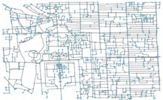
Figure 1. OSMnx graph for the downtown area of Beijing.

2.1. Determination of Alternate Routes

To illustrate how we formulate the problem, we focus on a subset of the T-Drive data set. Of the 10,357 cars in the data set, we select 418 of those that are traveling to or from the city center and the Beijing airport. In this specific scenario, the goal was to maximize traffic flow by redirecting a subset of the 418 cars to alternative routes such that the number of intersecting road segments is minimized. For this, optimizing over all cars simultaneously is required, which means that any redistribution of cars that resolves the original congestion must not cause a traffic jam anywhere else in the map. We used the OSMnx package to split the map of Beijing into segments and nodes and assign a unique ID to each. Our procedure can be summarized as follows:

1. Extract the road graph from the Beijing city map using OSMnx. This returns lists of segments and nodes with IDs. Nodes represent connections between segments, and segments are edges connecting the nodes, representing the streets (Figure 1).

2. Map the T-Drive trajectory data set cars’ GPS coordinates onto street segments in the graph, to determine the routes taken by the cars.

3. For each car, and each source and destination node, we extract all simple paths from source to destination and obtain 3 candidate alternative routes.² We use these 3 candidates as proposed alternative routes to redistribute traffic.

2.2. Formulating the Traffic Flow Optimization in QUBO Form

The definition of variables for the QUBO (equation (1)) requires some classical preprocessing on the input. In rare cases, it may not be possible to switch a car to different routes. For example, if there is no intersection or ramp near the car, it will not be considered for rerouting and will remain on its original path. Nevertheless, this car will still affect possible routings of other cars, so it is included in the QUBO. Figure 2 shows an example with road segments assigned to a car, as it is used in our workflow.

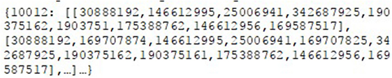
Figure 2. An example of a single car (with ID 10012) and its assigned routes, split into segments.

To optimize the traffic flow, we minimize the number of overlapping segments between assigned routes for each car. Thus, we formulate the optimization problem as follows: “Given 3 possible routes per car, which assignment of cars to routes minimizes the overall congestion on all road segments?” We require that every car should be assigned one of the 3 possible routes, while simultaneously minimizing total congestion over all assigned routes. It is important to emphasize that in this example each car was proposed 3 possible alternative routes—not the same set of 3 routes for all cars. This need not be the case in general; cars can have many possible routes. For simplicity, we take (maximum) 3 routes per car, because the mathematical description of the problem is identical regardless of the number of routes.

For every possible assignment of car to route, we define a binary variable q_ij representing car i taking route j. Because each car can only occupy one route at a time, exactly one variable per car must be true in the minimum of the QUBO. We define a constraint such that every car is required to take exactly one route. This can be formulated as the following constraint (assuming 3 possible routes):

simplified using the binary rule x² = x. As stated previously, routes are described by lists of street segments (S being the set of all street segments in the graph). Therefore, for every street segment sϵS, we identify all binary variables q_ij associated with routes that share street segment s (call this set B_s) and formulate the occupancy cost function:

For example, if route j₁ of car i₁, route j₂ of car i₂, and route j₃ of car i₃ share street segment s₁, then $B_{s_1}=\text{{}{q}_{i_1{j}_1},q_{i_2{j}_2},q_{i_3{j}_3}\text{}}$, and equation (3) takes the form:

In general, there can be many car/route variables q_ij that share some street segment s. equation (3) will then give a linear term for each of the binary variables (with a coefficient of +1) and a quadratic mixed term for every combination of two binary variables (with a coefficient of + 2). The global cost function for the QUBO problem, Obj from equation (1), can now be simply described by summing the cost functions for each street segment and the constraint from equation (2):

When summing components of the global cost function, the scaling parameter λ must be introduced. This ensures that equation (2) is satisfied for all cars in the minimum of the QUBO. To find this scaling factor, we find the maximum number of times some car i is present in cost functions of the form equation (3) and use this value as λ. This makes the cost of violating equation (2) greater than the cost of increasing the segment occupancy in every route by 1.

Now the cost function can be formulated as a quadratic, upper-triangular matrix, as required for the QUBO problem. We keep a mapping of binary variable q_ij to index in the QUBO matrix Q (as defined in equation (1)), given by I(q_ij). These indices are the diagonals of the QUBO matrix. The elements of the matrix are the coefficients of the q_ij terms in equation (5). To find these terms explicitly, whenever two routes j and j′ share a street segment s:

1. We add a (+1) at diagonal index I(q_ij) for every car i proposed with route j containing segment s.

2. We add a (+2) for every pair of cars i₁ and i₂ taking route j containing segment s at the off-diagonal element given by indices $I(q_{i{}_{1}j})$ and $I(q_{i_{2}j})$.

We then add the constraints to enforce that every car has only one route, as per equation (2):

1. For every car i with possible route j, we add (−λ) to the diagonal of Q given by index I(q_ij).

2. For every cross-term arising from equation (2), we add (2λ) to the corresponding off-diagonal term.

A special case occurs if a car is proposed only one route, meaning q_ij = 1. As stated previously, despite car i being assigned to route j, this assignment still affects other cars. This forces the quadratic constraint terms from equation (3) to be turned into additional linear terms: $2q_{ij}{q}_{i\mathrm{\prime }j\mathrm{\prime }}\to 2q_{i\mathrm{\prime }j\mathrm{\prime }}$. Additionally, by keeping a record of which routes every segment appears in, we can remove the redundant constraints, as some routes may overlap in more than one segment.

This results in a QUBO matrix as shown in Figure 3.

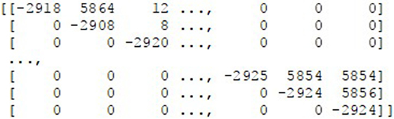
Figure 3. QUBO matrix describing the traffic flow problem.

2.3. Summary of the Traffic Flow Optimization Algorithm

Expressed as pseudo-code, the important high-level steps of the traffic flow optimization algorithm are as follows:

1. For each car i:

a. Determine the current route.

2. For each car i’s current route:

a. Map the source and destination to their nearest nodes in the road graph.

3. For each with source/destination pair:

a. Determine all simple paths from source to destination.

b. Find two alternative paths that are maximally dissimilar to the original route and to each other.

4. For each car i, define the set of possible routes needed to form the QUBO.

5. Define the matrix Q with binary variables q_ij as described in Section 2.2.

6. Solve the QUBO problem.

7. Update cars with the selected routes.

3. D-Wave Solvers and Architecture

Here, we briefly introduce the solvers and tools provided by D-Wave, to help understand how the problem was solved using the QPU.

3.1. Connectivity and Topology

The topology of the D-Wave 2X QPU is based on a C₁₂ Chimera graph containing 1,152 vertices (qubits) and over 3,000 edges (couplers). A Chimera graph of size C_N is an N × N grid of Chimera cells (also called unit tiles or unit cells), each containing a complete bipartite graph of 8 vertices (K_4,4). Each vertex is connected to its four neighbors inside the cell as well as two neighbors (north/south or east/west) outside the cell; therefore, every vertex has degree 6 excluding boundary vertices (King et al., 2015).

The 418-car example used 1,254 logical variables to represent the problem. A challenge in this scenario is the restricted connectivity between qubits on a D-Wave QPU, which limits the ability to directly solve arbitrarily structured problems. When using the D-Wave QPU directly, an interaction between two problem variables can only occur when there is a physical connection (coupler) between the qubits representing these variables. For most problems, the interactions between variables do not match the QPU connectivity. This limitation can be circumvented using minor embedding, a technique that maps one graph structure to another. The QPU we used has 1,135 functional qubits, thus it was not possible to embed the 1,254 logical variables on the QPU at once. Therefore, the problem was solved using the hybrid classical/quantum tool qbsolv (described in the next section).

3.2. The qbsolv Algorithm

In January 2017, D-Wave Systems open-sourced the software tool qbsolv (D-Wave Systems, 2017).³ The purpose of this algorithm is to provide the ability to solve larger QUBO problems, and with higher connectivity, than is currently possible on the QPU. Given a large QUBO input, qbsolv partitions the input into important components and then solves the components independently using queries to the QPU. This process iterates (with different components found by Tabu search) until no improvement in the solution is found. The qbsolv algorithm can optimize subproblems using either a classical Tabu solver or via submission to a D-Wave QPU. In this paper, we run qbsolv in the hybrid classical/quantum mode of submitting subproblems to the D-Wave 2X QPU.

The high-level steps performed by qbsolv in hybrid mode are as follows:

1. Find the largest clique⁴ that can be minor embedded in the QPU topology, or in the full Chimera graph if using the VFYC feature.⁵ This one-time operation can be done in advance.

2. Given a QUBO problem, initialize random bit string representing a solution to the problem.

3. Use a heuristic method to rank nodes according to importance; create a subproblem that fits on the QPU using the importance ranking.

4. Create subproblem using the importance order.

5. Solve subproblem by submitting it to the QPU and update variable states in the bit string.

6. Iterate steps 3–5 until no improvement in the objective function is found.

A full description of how the qbsolv algorithm works is detailed in Booth et al. (2017).

4. Results

The goal of these experiments was to map a real-world problem to a quantum annealing machine, which we have shown. When evaluating the solutions produced by the D-Wave QPU, the focus was on finding good quality solutions within short periods of calculation. To quantify the quality of a solution, we count the number of congested roads after optimization. Keeping in mind that routes are described by sets of road segments, we simply count the number of segments that appear in routes more than a given number of times (N_{intersections}). Here, we assume that a segment that appears in more than N_{intersections} routes will become congested. For this experiment, we chose N_{intersections} = 10.

To evaluate the QUBO formulation of the traffic flow problem, we designed the following experiment: for the 418 car QUBO problem (as presented in Section 2.2), we solved the problem 50 times using qbsolv. We also generated 50 random assignments of cars to routes as reference for the results. Intuitively, one would expect random route assignments to spread traffic across the alternative routes, thus reducing the number of congested segments. In Figure 4, we show the distribution of results (measured as the number of congested segments) after running the experiments using qbsolv and random assignments.

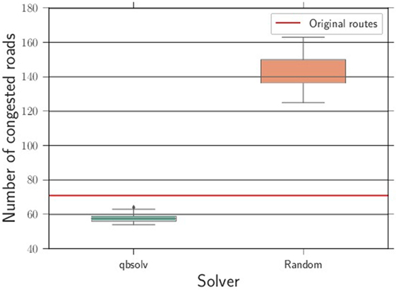
Figure 4. Results comparing random assignment of cars to routes, and qbsolv with calls to the D-Wave 2X QPU. The y-axis shows the distribution of number of congested roads. The red line is the number of congested roads given the original assignments of routes.

From the results in Figure 4, we can see that qbsolv redistributes the traffic over possible routes in a way that reduces the number of congested roads. This is evident both with respect to random assignment of routes and also shows improvement over the original assignment of routes. It should be noted that in the original assignment, there was a relatively small number of streets that are heavily occupied (meaning above the N_{intersections} = 10 threshold), as all the cars shared the same route, and that the average occupancy was much higher than N_{intersections} = 10. It is also worth noting that all 50 experiments using qbsolv resolved the congestion.

Additionally, we measured the performance of qbsolv as a function of its run time. The qbsolv source code was compiled and executed on a server in Burnaby, Canada, to minimize the latency between submitting jobs to the QPU and obtaining the results. However, since the QPU used was a shared resource via the cloud, run time of qbsolv varied greatly. Therefore, we consider the run time of qbsolv to be the minimum of the observed run times, as this represents most faithfully the algorithm, independent of the load on the D-Wave system. This run time was observed as 22 s. There is also no evidence of correlation between the run time of qbsolv and performance (the long run times are due to waiting in the job submission queue). Given the performance results of qbsolv, it is reasonable to assume that a dedicated D-Wave QPU (circumventing the public job submission queue) could be suitable for these kinds of optimization problems. A visual showing the traffic density on the Beijing road graph before (original routes) and after optimization (using qbsolv) is shown in Figure 5.

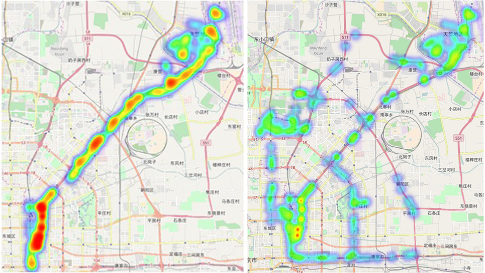
Figure 5. Left: Unoptimized situation under consideration of cars causing traffic jam in the network. Right: Optimized redistributed cars using qbsolv. Note that the areas in red, which indicate high traffic density, are mostly absent from the right picture.

5. Conclusion and Future Work

The currently presented problem is a simplified version of traffic flow, as it incorporates only a limited set of cars, no communication to infrastructure, no other traffic participants, and no other optimization targets except minimization of road congestion. In our future work, we intend to consider all of these parameters and will also need to consider creative ways of formulating these parameters as part of the QUBO problem. We will continue to focus on solving real-world problems by means of quantum machine learning, quantum simulation, and quantum optimization. Furthermore, we find that these types of real-time optimization problems are well-suited for the D-Wave systems and the hybrid tools that use them. The more combinatorially complex the problem becomes, the more time would be needed for classical algorithms to consider additional parameters. However, D-Wave QPUs have historically grown in number of qubits from one generation to the next, and given that this trend is likely to continue, it is reasonable to assume that obtaining high-quality solutions quickly using the QPU will be sustainable moving forward. We expect that in future generations of QPUs, we will be able to embed larger problems directly. This will allow us to further leverage the performance of the QPU.

Author Contributions

All authors contributed to the creation of this paper.

Conflict of Interest Statement

The authors are a collaboration between Volkswagen and D-Wave Systems employees.

Acknowledgments

The authors thank the Volkswagen Group for its support in this exploratory research project. Further to the authors thank the team at D-Wave Systems, especially Murray Thom, Adam Douglass, and Andy Mason.

Footnotes

References

Boeing, G. (2017). Osmnx: new methods for acquiring, constructing, analyzing, and visualizing complex street networks. Comput. Environ. Urban Syst. 65, 126–139. doi: 10.1016/j.compenvurbsys.2017.05.004
Booth, M., Reinhardt, S. P., and Roy, A. (2017). Partitioning Optimization Problems for Hybrid Classical/Quantum Execution. Available at: https://www.dwavesys.com/resources/publications
Denchev, V. S., Boixo, S., Isakov, S. V., Ding, N., Babbush, R., Smelyanskiy, V., et al. (2016). What is the computational value of finite-range tunneling? Phys. Rev. X 6, 031015. doi:10.1103/PhysRevX.6.031015
D-Wave Systems. (2017). D-Wave Initiates Open Quantum Software Environment. Available at: https://www.dwavesys.com/press-releases/d-wave-initiates-open-quantum-software-environment
Johnson, M. W., Amin, M. H. S., Gildert, S., Lanting, T., Hamze, F., Dickson, N., et al. (2011). Quantum annealing with manufactured spins. Nature 473, 194–198. doi:10.1038/nature10012
King, J., Yarkoni, S., Nevisi, M. M., Hilton, J. P., and McGeoch, C. C. (2015). Benchmarking a Quantum Annealing Processor with the Time-to-Target Metric. arXiv:1508.05087.
Lanting, T., Przybysz, A. J., Smirnov, A. Y., Spedalieri, F. M., Amin, M. H., Berkley, A. J., et al. (2014). Entanglement in a quantum annealing processor. Phys. Rev. X 4, 021041. doi:10.1103/PhysRevX.4.021041
Los Alamos National Laboratory. (2016). D-Wave Rapid Response. Available at: http://www.lanl.gov/projects/national-security-education-center/information-science-technology/dwave/
Lucas, A. (2014). Ising formulations of many np problems. Front. Phys. 2:5. doi:10.3389/fphy.2014.00005
O’Gorman, B., Babbush, R., Perdomo-Ortiz, A., Aspuru-Guzik, A., and Smelyanskiy, V. (2015). Bayesian network structure learning using quantum annealing. Eur. Phys. J. Spec. Top. 224, 163–188. doi:10.1140/epjst/e2015-02349-9
Perdomo-Ortiz, A., Fluegemann, J., Narasimhan, S., Biswas, R., and Smelyanskiy, V. (2015). A quantum annealing approach for fault detection and diagnosis of graph-based systems. Eur. Phys. J. Spec. Top. 224, 131–148. doi:10.1140/epjst/e2015-02347-y
Raymond, J., Yarkoni, S., and Andriyash, E. (2016). Global warming: temperature estimation in annealers. Front. ICT 3:23. doi:10.3389/fict.2016.00023
Rieffel, E. G., Venturelli, D., O’Gorman, B., Do, M. B., Prystay, E. M., and Smelyanskiy, V. N. (2015). A case study in programming a quantum annealer for hard operational planning problems. Quantum Info. Process. 14, 1–36. doi:10.1007/s11128-014-0892-x
Venturelli, D., Mandrà, S., Knysh, S., O’Gorman, B., Biswas, R., and Smelyanskiy, V. (2015a). Quantum optimization of fully connected spin glasses. Phys. Rev. X 5, 031040. doi:10.1103/PhysRevX.5.031040
Venturelli, D., Marchand, D. J. J., and Rojo, G. (2015b). Quantum Annealing Implementation of Job-Shop Scheduling. arXiv:1506.08479.
Yuan, J., Zheng, Y., Xie, X., and Sun, G. (2011). “Driving with knowledge from the physical world,” in Proceedings of the 17th ACM SIGKDD International Conference on Knowledge Discovery and Data Mining, KDD ’11 (New York, NY: ACM), 316–324.
Yuan, J., Zheng, Y., Xie, X., and Sun, G. (2013). T-drive: enhancing driving directions with taxi drivers’ intelligence. IEEE Trans. Knowl. Data Eng. 25, 220–232. doi:10.1109/TKDE.2011.200
Zheng, Y. (2011). T-Drive Trajectory Data Sample. Available at: https://www.microsoft.com/en-us/research/publication/t-drive-trajectory-data-sample/
Keywords: optimization, quantum annealing, traffic flow, quantum computing, optimization algorithms
Citation: Neukart F, Compostella G, Seidel C, von Dollen D, Yarkoni S and Parney B (2017) Traffic Flow Optimization Using a Quantum Annealer. Front. ICT 4:29. doi: 10.3389/fict.2017.00029
Received: 08 August 2017; Accepted: 06 December 2017;
Published: 20 December 2017
Edited by:
Shiro Kawabata, National Institute of Advanced Industrial Science and Technology, JapanCopyright: © 2017 Neukart, Compostella, Seidel, von Dollen, Yarkoni and Parney. This is an open-access article distributed under the terms of the Creative Commons Attribution License (CC BY). The use, distribution or reproduction in other forums is permitted, provided the original author(s) or licensor are credited and that the original publication in this journal is cited, in accordance with accepted academic practice. No use, distribution or reproduction is permitted which does not comply with these terms.
*Correspondence: Florian Neukart, florian.neukart@vw.com