Development of maps of simple and complex cells in the primary visual cortex
- 1 Institute for Adaptive and Neural Computation, University of Edinburgh, Edinburgh, UK
- 2 Department of Neuroscience, Physiology and Pharmacology, University College London, London, UK
- 3 Unité de Neurosciences Information et Complexité, CNRS, Gif-sur-Yvette, France
Hubel and Wiesel (1962) classified primary visual cortex (V1) neurons as either simple, with responses modulated by the spatial phase of a sine grating, or complex, i.e., largely phase invariant. Much progress has been made in understanding how simple-cells develop, and there are now detailed computational models establishing how they can form topographic maps ordered by orientation preference. There are also models of how complex cells can develop using outputs from simple cells with different phase preferences, but no model of how a topographic orientation map of complex cells could be formed based on the actual connectivity patterns found in V1. Addressing this question is important, because the majority of existing developmental models of simple-cell maps group neurons selective to similar spatial phases together, which is contrary to experimental evidence, and makes it difficult to construct complex cells. Overcoming this limitation is not trivial, because mechanisms responsible for map development drive receptive fields (RF) of nearby neurons to be highly correlated, while co-oriented RFs of opposite phases are anti-correlated. In this work, we model V1 as two topographically organized sheets representing cortical layer 4 and 2/3. Only layer 4 receives direct thalamic input. Both sheets are connected with narrow feed-forward and feedback connectivity. Only layer 2/3 contains strong long-range lateral connectivity, in line with current anatomical findings. Initially all weights in the model are random, and each is modified via a Hebbian learning rule. The model develops smooth, matching, orientation preference maps in both sheets. Layer 4 units become simple cells, with phase preference arranged randomly, while those in layer 2/3 are primarily complex cells. To our knowledge this model is the first explaining how simple cells can develop with random phase preference, and how maps of complex cells can develop, using only realistic patterns of connectivity.
1 Introduction
The early studies of Hubel and Wiesel(1962, (1968) identified two functionally different classes of cells in cat and monkey primary visual cortex, which they called “simple” and “complex.” Simple-cells respond to a drifting sinusoidal grating only when the peaks and troughs of the sine wave are precisely aligned with the on and off subregions of the cell’s receptive field (RF). On the other hand, the response of complex cells is largely phase invariant, so the cell will respond to most or all phases of a sine grating, while remaining orientation selective. Previous studies have shown a relationship between cortical depth and the prevalence of the two cell classes (Ringach et al., 2002; Hirsch and Martinez, 2006). Hirsch and Martinez (2006) argued that in cat, neurons with simple RFs are only found in layer 4 and upper layer 6, the layers that primarily receive direct thalamic input. Data from macaque monkey are not as clear, but show a similar trend with predominantly simple cells in layer 4 to complex-cells dominating in layer 2/3 (Ringach et al., 2002).
Over the years, three main types of model circuits leading to phase invariance have been proposed: hierarchical, parallel, and recurrent (Martinez and Alonso, 2003). As Martinez and Alonso (2003) pointed out, these three classes of models are becoming remarkably similar to each other as additional connectivity is being added to account for new physiological constraints. Regardless of which of the three classes of models is closest to reality, a fundamental question still remains largely unanswered: How does the specific and precise circuitry (assumed by each of these theories) develop? One possible explanation is that initially homogeneous or stochastic cortical connectivity can be modified by activity dependent-mechanisms in such a way that, over time, adult connectivity patterns emerge (von der Malsburg, 1973; Willshaw and von der Malsburg, 1976; Nagano and Kurata, 1981). This self-organization can be driven by intrinsic spontaneous neural activity, external visual stimuli, or both.
Another feature of the primary visual cortex whose development is often explained by self-organization is its functional topographic organization. The best known examples of topographically organized functional features are retinotopy, ocular dominance, and orientation preference. In this work we will focus on the organization of orientation and phase, the two defining characteristics for simple and complex cells. Orientation preference maps are present throughout all cortical layers in cat and monkey, and are aligned, meaning that when one traverses the visual cortex perpendicularly to the surface one will find neurons with a similar position and orientation preference (Hubel and Wiesel, 1974). Recent two-photon imaging studies in cat (Ohki et al., 2005) have shown that the orientation maps in superficial layers are smooth with single-cell resolution. Numerous models have been proposed to account for the development of orientation maps in the primary visual cortex (Miller, 1994; Shouval et al., 2000; Miikkulainen et al., 2005; Ringach, 2007; Grabska-Barwinska and von der Malsburg, 2008).
The spatial organization of absolute phase preference is much less clear. For a fixed eye position and display screen, the absolute phase preference of a neuron is the phase of the sine grating that elicits the strongest response from the neuron. A study in cat (Liu et al., 1992) found that nearby neurons tend to have opposite absolute phase preferences, whereas a study in macaque (Aronov et al., 2003) found that nearby neurons tend to have correlated absolute phase preference. Furthermore, relative phase, which describes the alignment of the ON and OFF RF subfields with respect to the center of RF, was found not to cluster in cat V1 (DeAngelis et al., 1999). It is important to note that findings about relative phase do not transfer to absolute phase, as it is possible that two neurons with opposite relative phase could still have highly overlapping ON and OFF RF subregions due to local scatter of RF centers. Despite this ongoing controversy about the organization of phase in visual cortex, we believe that the above studies clearly show that the representation of phase in V1 is significantly more disordered than that of orientation, and consequently that one can expect a variety of phases to be represented in each local region of cortex. As we are primarily interested in absolute phase in this work, for the sake of brevity, we will refer to the absolute phase as simply “phase” in the remainder of this paper.
The main goal of this study is to reconcile the development of orientation maps with the development of complex cells in V1. This is an important and non-trivial problem for the following reason: a natural way to construct complex cells is to let them group responses from simple cells with the same orientation preference, but with different phase preferences (Hubel and Wiesel, 1962). Because, as discussed above, proximate simple cells are selective to a variety of phases but similar orientations, such grouping can easily be achieved in the visual cortex by simply pooling responses from nearby simple-cells indiscriminately (see Figure 1). However, most current models of map development are driven by various analogs of Hebbian learning and Mexican-hat-like lateral interactions, which ensure that nearby neurons develop highly correlated RFs, as will be explained in greater detail in “Section 1.1.” Yet two RFs of the same orientation but opposite phase are perfectly anti-correlated, and thus will not be grouped together by such models. This makes it very hard for these models to explain the formation of complex cells. We will show how Hebbian models can nevertheless lead to locally diverse phase preferences and thus complex cells, when the model architecture is sufficiently realistic.
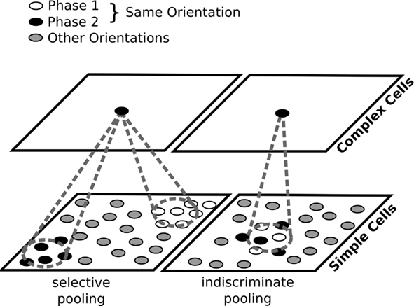
Figure 1. Two possible ways to construct complex cells by pooling outputs of simple cells. Left: in most previous models of map development, neurons with similar orientation preferences but different phase preferences are widely separated in the map. For a complex cell to achieve a phase invariant but orientation-selective response, it will need to pool responses of simple cells of corresponding orientation preference located at several different positions in the map. Right: if phase is locally variable, complex cells can simply indiscriminately pool from a narrow region of the map. Locally variable phase ensures that each complex cell will receive inputs from simple-cells selective to a range of phases, while the smoothness of the orientation map will ensure that those simple cells have similar orientations. For the sake of clarity, in this figure, we approximate the continuous range of possible phases with just two.
Furthermore, in this study we address an additional discrepancy between previous developmental models of map formation and known cortical anatomy. In models that are based on lateral interactions as the driving force for map development (Olson and Grossberg, 1998; Shouval et al., 2000; Hyvärinen and Hoyer, 2001; Miikkulainen et al., 2005), the extent and relative strengths of the lateral and afferent interactions are very important parameters. There is, however, substantial evidence suggesting that the strongest source of lateral interactions is the lateral connections originating from pyramidal neurons in layer 2/3 (Binzegger et al., 2004, 2009; Chisum and Fitzpatrick, 2004; Hirsch and Martinez, 2006). Despite these experimental results, all previous models for orientation preference map development that we are aware of that depend on the plasticity of V1 afferent connections from LGN place the long-range lateral connectivity in an analog of layer 4C. That is, the layers with long-range connections in these models receive direct input from the LGN, and they develop simple cells. Thus, previous models are in conflict with the available experimental evidence.
Here we introduce a Hebbian model of simple and complex-cell development that results in matching orientation maps in both simple and complex-cell layers, disorder in the spatial arrangement of simple cells with similar phase preferences, and realistic orientation and phase tuning curves for both simple and complex cells. At the same time, the model follows the established anatomical constraints of the connectivity in cortical layer 4C and 2/3, and does not assume any specific neuron-to-neuron connectivity at the beginning of development, an improvement over the previous models of complex-cell map development.
The model contains two topographically ordered sheets of V1 cells, one representing cortical layer 4Cβ and one representing layer 2/3, with only layer 4Cβ receiving direct thalamic input. The self-organization of maps is achieved by short-range excitatory and long-range inhibitory connections in both sheets, modeling the net inhibitory interactions for high contrast stimuli at large distances (Miikkulainen et al., 2005; Law, 2009). The most important novel feature of the model is that the lateral connections in the sheet corresponding to layer 4Cβ are several times weaker than those in layer 2/3, making the layer 2/3 lateral interactions the major driving force of map development. Importantly, there is strong anatomical evidence that this is the configuration in macaque V1 (Binzegger et al., 2004, 2009; Chisum and Fitzpatrick, 2004; Hirsch and Martinez, 2006). We are not aware of any previous model of orientation map development that follows this constraint. At the same time, this arrangement is one of the key features of the model, because making the lateral connectivity weaker in the sheet representing layer 4Cβ takes away the direct self-organization pressure from layer 4Cβ. The weaker lateral connectivity in layer 4Cβ combined with two realistic sources of variability we introduce into the model (initial local retinotopical scatter and intrinsic activity noise) allows disordered phase preference to develop in the 4Cβ sheet. The resulting disordered phase preference can then be utilized by the units in layer 2/3, which pool the responses of simple cells in layer 4Cβ via narrow afferent connectivity patterns to produce complex-cell-like RFs. In order to ensure development of RFs in layer 4Cβ and development of matching maps in both layer 4Cβ and 2/3, the model also contains feedback connectivity from layer 2/3 to layer 4Cβ, which corresponds to the known strong interlaminar pathway starting in layer 2/3 and reaching back to layer 4 via layers 5 and 6 (Binzegger et al., 2004; Hirsch and Martinez, 2006).
This model demonstrates for the first time that it is possible to develop a map of complex cells using only known mechanisms and anatomical features of primate V1, unlike previous models (discussed in the next section). Furthermore, the model produces realistic single-cell properties, such as realistically shaped orientation tuning curves for both simple and complex neurons. The specific connectivity that develops in the model also allows us to formulate predictions: First, we predict clustering of the (albeit weak) phase preference of complex cells in layer 2/3, and second we predict a relationship between modulation ratios (MR) and the position of cells in the orientation maps.
Finally, in the proposed model we simulate both pre-natal and post-natal developmental phases, driven by retinal waves before eye opening and then by natural images. The simple and repetitive patterns of retinal waves help to establish initial smooth orientation maps, reducing the dependence on the less predictable patterns of natural image stimulation. Simulating them also helps the model account for findings that orientation maps are present even at eye opening (Chapman et al., 1996; Crair et al., 1998). However, the retinal waves do not play a critical role in this model, and just like with previous models in the LISSOM family (Miikkulainen et al., 2005), it should also be possible to adjust the model such that it can show development of maps driven purely by natural stimuli. In any case, the retinal waves as implemented here represent an advance over previous models of pre-natal development. Many of those models have assumed anti-correlated activities between ON and OFF LGN channels, as is true in normal vision. However, retinal waves activate both ON and OFF retinal ganglion cells nearly simultaneously (Kerschensteiner and Wong, 2008), implying that the activation patterns between ON and OFF LGN cells with the same retinotopic preference will be highly correlated during pre-natal development. In the proposed model we simulate retinal waves that activate both ON and OFF channels at the same time. As will be discussed in further detail in “Section 2.1,” by assuming randomized relative strength of connections from ON and OFF LGN sheets to individual layer 4C model neurons – as recently found for the macaque (Yeh et al., 2009) – we show that initial orientation map development can be driven by this more realistic simulation of retinal waves. The model thus represents a novel and more realistic simulation of how retinal waves or other spontaneous activity could drive initial development of orientation maps.
1.1 Related Models
One of the first studies to demonstrate how complex-cell-like properties can emerge from stimulus-driven self-organization was the work of Földiák (1991), which introduced a local learning rule (trace rule) that developed complex-cell RFs when trained with a temporal sequence of smoothly translating bars. Einhäuser et al. (2002) showed that a two-layer network using a competitive Hebbian learning rule can develop the properties of complex cells, when trained on natural images. A recent model by Karklin and Lewicki (2008) develops complex cells by learning the statistical distributions that characterize local natural image regions. None of these models, however, can explain the emergence of functional topological organization, such as orientation maps, which is important because of the striking difference between the observed organizations for phase and for orientation.
Sullivan and de Sa (2004) address the problem of complex-cell map development by combining Földiák’s trace rule with a self-organizing map algorithm. Their model consists of two layers of neurons. The first layer is a fixed sheet containing hardwired simple cells with various orientation and position preferences. The cells in the second layer are fully connected to the cells in the first layer and adapt their afferent connections based on a combination of Hebbian, winner takes all and trace rules. When stimulated with oriented moving stimuli, this model develops RFs that are invariant to position but selective to orientation, and also ensures that nearby neurons have similar orientation preferences. The main drawback of this model is that it does not explain how orientation maps and disordered phase representation can develop in the layer containing simple cells; it assumes that these have already developed, and explaining this process is not trivial as argued in the previous section.
So far, there have been three models showing how maps of simple cells with disordered phase preference and correspondingly organized maps of complex cells can develop. In order to understand the contributions of these models it is helpful to emphasize the main underlying problem, which is how to reconcile the development of disordered phase preference with the typically Mexican-hat-like lateral interactions that drive nearby cells to develop correlated RFs. Because simple cells are strongly phase selective, two simple-cells preferring the same orientation but opposite phases will respond in an anti-correlated manner when presented with a range of sinusoidal gratings of the same orientation but varying phases. This means that any self-organizing rule forcing nearby neurons to develop correlated RFs will not allow cells selective to opposite phase to develop next to each other, in contradiction with the observed disordered phase preference (Figure 2 left).
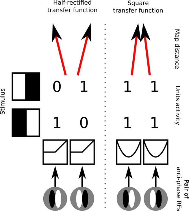
Figure 2. Demonstration of the underlying conflict between disordered phase preference, development of simple cells, and Mexican-hat-like lateral interactions. Left, RFs for an example pair of simple cells with half-rectified activation functions that are selective to the same orientation but opposite phase. When such cells are presented with stimuli of preferred orientation, they will have mutually anti-correlated activities. Mexican-hat-like lateral interactions constrain nearby neurons to have highly correlated activities, and will thus cause neurons selective for the same orientation but opposite phase to develop in different map locations. Right, an example configuration that resolves this conflict by applying a squaring transfer function to the response of the simple cells, which relies on the neurons somehow maintaining a “negative activation” internally, mapping both strong positive and strong negative activations to a strong output level. This ensures that the activity of neurons will become correlated and thus allows them to occupy nearby locations in the map, but renders their output non-simple-cell-like, and is not based on any known neural mechanism.
One way to overcome this problem, allowing neurons selective to opposite phases to develop nearby, is to map the responses of phase opposite cells to the same values, and then apply the lateral interactions (or mechanisms analogous to them) over this transformed representation. A simple and elegant, albeit not biologically plausible, way to achieve this is to allow neurons to have signed responses rather than only positive “firing rates.” That is, the response of an idealized neuron preferring phase a, to a sinusoidal stimulus of phase a + π, will be −1. One can then pass activities of such neurons through a squaring function that ensures that the responses of each neuron to its preferred phase and anti-phase are equal (Figure 2 right). However, this approach is arguably just a mathematical trick, as it is not clear how to link the negative activities and the squaring operation to any known neural mechanisms.
There have been two studies that have used this trick to achieve development of disordered phase preference, complex cells and topographic maps. First, Hyvärinen and Hoyer (2001) employed a hierarchical two-layer model where signed units with simple-cell-like RFs emerge in the first layer. The second layer contains units that locally pool squared activations of units in the first layer. A topographic extension of the independent component analysis (ICA) learning rule is used to self-organize the model, and leads to the development of orientation maps. Due to the signed responses of simple cells and the squaring of their output, this learning rule also ensures disordered phase preference representation across the simple cells, which in turn ensures that units in the second layer, which simply pool local activities from the first layer, become complex cells.
Similarly, Weber (2001) uses a two-layer model, with the first layer containing “feature cells” with bottom up and top down weights. During training, these cells are allowed to have negative responses that are then squared. The second layer contains “attractor cells,” with lateral weights, which become complex cells. The feature cells in this model are trained with a sparse coding algorithm and develop orientation preference, orientation maps, and disordered phase preference.
Neither Weber (2001) nor Hyvärinen and Hoyer (2001) propose a biological circuit that could implement their algorithms. Overall, this lack of grounding in cortical anatomy is the main limitation of the Hyvärinen and Hoyer (2001) and Weber (2001) probabilistic models. As Hyvärinen and Hoyer (2001) mention, these models represent the combined effect of evolution, pre-natal, and post-natal development. Therefore it is not possible to say which properties of the model correspond to putatively hardwired architecture of cortical connections, and which to activity-based adaptive mechanisms. Furthermore, the simulations in both studies were performed with small sheets of neurons because of the very high computational requirements of the models, which prevents assessment of the smoothness and regularity of the developed orientation maps in comparison with experimental maps.
As we have noted above, the idea of squaring negative activations of neurons is not biologically plausible. Olson and Grossberg (1998) address this problem by assuming instead specifically hardwired ensembles of neurons, which they call dipoles, each with only positive activations. Each such dipole consists of two pairs of neurons that strongly inhibit each other, and thus will have anti-correlated activities during development. The BCM learning rule used in their study ensures that in each dipole the two pairs of neurons will develop RFs selective to opposite phases. In this way, a dipole has a role analogous to that of the signed units with squaring in the previous two studies. Similarly to the above studies, the model of Olson and Grossberg (1998) consists of two layers, the first containing the ensembles of simple cells (dipoles). The dipoles are laterally connected via short-range excitatory and long-range inhibitory connections that drive map formation in the first layer. This in turn allows modeling of complex cells in the second layer as units that simply pool the activations from simple cells via Gaussian afferent connections. The main limitation of this model is that it requires arbitrary specific wiring between pairs of simple cells at the beginning of the simulation. Currently, there is no evidence for this particular pattern of highly specific connectivity in undeveloped primary visual cortex. Furthermore, the model does not show how strong orientation-selective responses for complex cells can develop, because the model’s complex cells have elevated responses to all orientations. Also, the authors do not present orientation maps in the complex layer, preventing comparison with animal maps and with their simple-cell layer maps. Experimental evidence suggests simple and complex cells within a column should exhibit similar orientation preferences (Blakemore and Price, 1987).
In this study we present a model of complex cell map development that does not rely on negative activations or arbitrary pre-specified connectivity. Instead, the key idea is to weaken the lateral interactions in the layer that is – after development – predominantly occupied by simple cells, moving the strong lateral connections to the layer that is occupied by complex cells, in line with experimental evidence. This means that nearby simple cells are not forced to develop correlated phase response, as complex cells are not strongly selective to phase and the activity of simple cells is not directly shaped by the strong lateral interactions.
2 Materials and Methods
2.1 Model Architecture
The model was built using the freely available Topographica simulator (Bednar, 2009) and is loosely based on the LISSOM architecture (Miikkulainen et al., 2005). The main modifications are: a new sheet of neurons corresponding to layer 2/3, decreased the strength of lateral connectivity in the sheet corresponding to layer 4C, continuous network dynamics between input presentations, more realistic pre-natal retinal and LGN processing, and additional sources of variability in the architecture and responses (see Figure 3). A model sheet corresponds to a rectangular portion of a continuous 2D plane and contains a 2D array of firing rate single-compartment neural units. Dimensions are defined in sheet coordinates rather than numbers of units, so that parameter values are independent of the number of units in any particular simulation (Bednar et al., 2004).
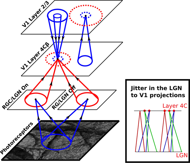
Figure 3. The model architecture. Each circular dot in this diagram represents a single unit in the indicated sheet of neurons. For each dot the cones indicate incoming projections from other sheets, and the dashed circles indicate a set of lateral connections to that unit within the same sheet. Arrows on the projection cones indicate the flow of information and red color indicates plastic connections whereas blue indicates connections that are not modified during development. The activity propagates from the photoreceptors to LGN ON and OFF sheets, and from there to the cortical layer 4Cβ. Within layer 4Cβ, activity spreads laterally via short-range excitatory and medium-range inhibitory lateral connections. Activity from layer 4Cβ further propagates via narrow afferent connectivity to layer 2/3, where it can again spread laterally via short-range excitatory and long-range inhibitory lateral connections. Finally, activity propagates back from layer 2/3 to layer 4Cβ via narrow excitatory and wider inhibitory connections, in a recurrent loop that (in combination with lateral connections in layer 4Cβ and 2/3) settles activity into stable “blobbs” in layer 2/3. In layer 4Cβ, activities settle into regions co-localized with the “blobbs” in layer 2/3, but in which only some neurons are activated. This difference between the activation patterns in layer 2/3 and 4Cβ is mainly due to the weaker lateral connectivity in layer 4Cβ, which does not force nearby neurons to be co-activated. See “Section 2.2” for a more detailed description of the network dynamics.
The simulator operates in discrete time steps. Retinal input changes every 20 time steps (and during this period is kept constant), and therefore afferent inputs to the layer 4Cβ sheet are effectively updated every 20 steps. Due to the recurrent connections, activities in the cortical sheets are updated in each simulation step. This represents a discrete simulation of an otherwise continuous process of changes in membrane potential due to incoming spikes and consequent generation of spikes. Due to the recurrent connections, discrete simulation of this process can create or amplify oscillation in the network. Therefore, as will be described in greater detail below, in the new model we smooth out the neural dynamics, by computing the present activity of the model neuron as an interpolation between its previous activity, and the newly computed activity. This process allows a lower time resolution to be used, making these otherwise intractable simulations feasible.
The Topographica simulator is based on 2D sheets of computational elements (neurons), referenced by a coordinate system we will refer to as sheet coordinates, where the central sheet element corresponds to coordinates (0, 0). The number of units simulated in each sheet is determined by setting the density of units per unit length in both sheet dimensions. Both V1 sheets have nominal dimensions 1.0 × 1.0. The size of the RGC/LGN (2.0 × 2.0) and photoreceptor (2.75 × 2.75) sheets was chosen to ensure that each unit in the receiving sheet has a complete set of connections, thus minimizing edge effects in the RGC/LGN and V1 sheets. The density of units per 1.0 × 1.0 area is 48 × 48 for the photoreceptor and RGC/LGN ON and OFF sheets, and 96 × 96 for both cortical sheets.
The ON/OFF units are called RGC/LGN units for simplicity, although they represent the entire pathway between the retinal photoreceptors and V1, including the retinal ganglion cells, LGN cells, and the connection pathways. The activation level for a unit at position j in an RGC/LGN sheet at time t is defined as:
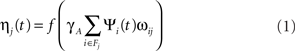
the activation function f is a half-wave rectifying function that ensures positive activation values, ψi is the activation of unit i taken from the set of neurons on the retina from which RGC/LGN unit j receives input (its connection field Fj), ωij is the connection weight from unit i in the retina to unit j in the RGC/LGN, and γA is a constant positive scaling factor that determines the overall strength of the afferent projection. Retina to RGC/LGN weights in the ON and OFF channels are set to fixed strengths with a difference-of-Gaussians kernel (σcenter = 0.07, σsurround = 0.2, in sheet dimensions), with ON connection fields having a positive center and negative surround and vice versa for OFF connections (Miikkulainen et al., 2005).
Units in the cortical sheets each receive up to three types of projections represented as matrices of weights: afferent, lateral, and feedback (Figure 3). The contribution Xjp to the activation of unit j in the layer 4Cβ sheet or layer 2/3 sheet from each projection p at time t is given by:
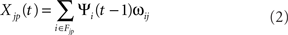
where ψi(t) is the activation of unit i taken from the set of neurons in the input sheet of projection p from which unit j receives input (its connection field Fjp), and ωij is the connection weight from unit i in the input sheet of projection p to unit j in the output sheet of projection p. All connection field weights are initialized with uniform random noise multiplied by a 2D Gaussian profile, cut-off at the distance specified below. Contributions from each projection are weighted and summed to form the overall input to unit i:
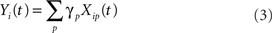
where γp is a constant determining the sign and strength of projection p. Table 1 shows the strength, initial Gaussian kernel spatial extent, and the cut-off distance values for all projections. The final output of unit i is computed as:

where
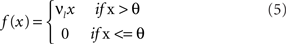
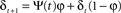
and where λ = 0.3 is a time-constant parameter that defines the strength of smoothing of the recurrent dynamics in the network. ε is a normally distributed zero mean random variable, which corresponds to firing rate fluctuations, and νl is the gain of neurons in layer l. To facilitate a smooth transition between pre-natal and post-natal development we implement a simple homeostatic plasticity mechanism for neurons in layer 4Cβ, leaving θ constant for neurons in layer 2/3. For neurons in layer 4Cβ, θ is adapted according to the following equation:

where ξ = 0.02 is the time constant of the threshold adaptation, μ = 0.003 is a constant defining the target average activity, θ = 0.9 and δ is the recent average activity of the neuron:
where φ = 0.002 is the time constant of the activity averaging and ψ(t) is the activity of the given neuron at time t.
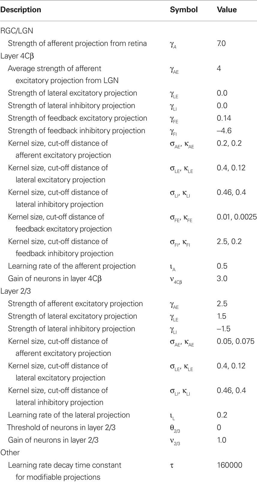
Table 1. Model parameters.
Because the initial connection weights from the RGC/LGN neurons to neurons in layer 4Cβ sheet have a 2D Gaussian profile multiplied with uniform random noise, the neuron will initially respond strongly when a stimulus is presented in the center of its RF. If the retinotopic ordering of RF centers were perfect, activities of nearby neurons would be highly correlated, preventing the development of disordered phase. Instead we assume that the initial activity of neurons will be more variable, because the initial retinotopic wiring between LGN and V1 is locally imperfect. Starting from perfect retinotopic wiring from RGC/LGN to layer 4Cβ, we offset the afferent connection fields of each layer 4Cβ neuron by a random factor drawn from a Gaussian distribution with variance σ = 0.25, which is similar to the size of the afferent connection fields of the layer 4Cβ neurons (see Figure 3; Table 1). RF position scatter at the scale of RF size has been reported in experimental studies (Warren et al., 2001; Buzás et al., 2003).
2.2 Learning
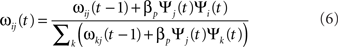
Four projections in the model are modified during development: the afferent projections from the two RGC/LGN sheets to the layer 4Cβ sheet, and the inhibitory lateral connections in both cortical sheets. The other projections all have narrow connection fields that typically do not show significant structural changes due to learning. In order to save computational resources, connection weights in the modified projections are adjusted only every 20 time steps at the end of each input presentation. Weights from unit i to unit j are adjusted by unsupervised Hebbian learning with divisive normalization:
where βp is the Hebbian learning rate for the connection fields in projection p, and k ranges over all neurons making a connection of this same type (afferent, lateral excitatory, lateral inhibitory, feedback excitatory, or feedback inhibitory). That is, weights are normalized jointly by type, with excitatory and inhibitory connections normalized separately to preserve a balance of excitation and inhibition, and lateral and feedback connections normalized separately from afferent to preserve a balance between feed-forward and recurrent processing. Learning rate parameters are specified as a fixed value ιp for each projection, and then the unit-specific values used in the equation above are calculated as βp = ιp/υp, where υp is the number of connections per connection field in projection p. We apply an exponential decay to the learning rates for the four modified projections throughout the simulation, simulating the decrease in plasticity of maturing V1. The reader can see the initial values of learning rate parameters and corresponding rates of decay in Table 1.
2.3 Input Patterns
In the simulation we consider both the pre- and post-natal stages of development (illustrated in Figure 4), each lasting 100000 time steps. In the first stage the input patterns correspond to spatially correlated spontaneous visual system activity, such as the retinal waves generated in the retina of young animals (Wong, 1999). We model these patterns as expanding rings of activity convolved with white noise, representing the moving edge of a retinal wave, analogously to how cortical waves have been modeled previously (Grabska-Barwinska and von der Malsburg, 2008; see Figure 4 top panel). The second stage models post-natal visual experience (see Figure 4 bottom panel). The natural images are retina-sized patches extracted from movies of natural environment, kindly provided by Kayser et al. (2003). For each natural image presentation, a random sub-image of the same dimensions as the photoreceptor sheet was selected. Each pixel value in the sub-image is converted into a real value in the range of 0–1.0 and the corresponding units in the photoreceptor sheet are set to these values.
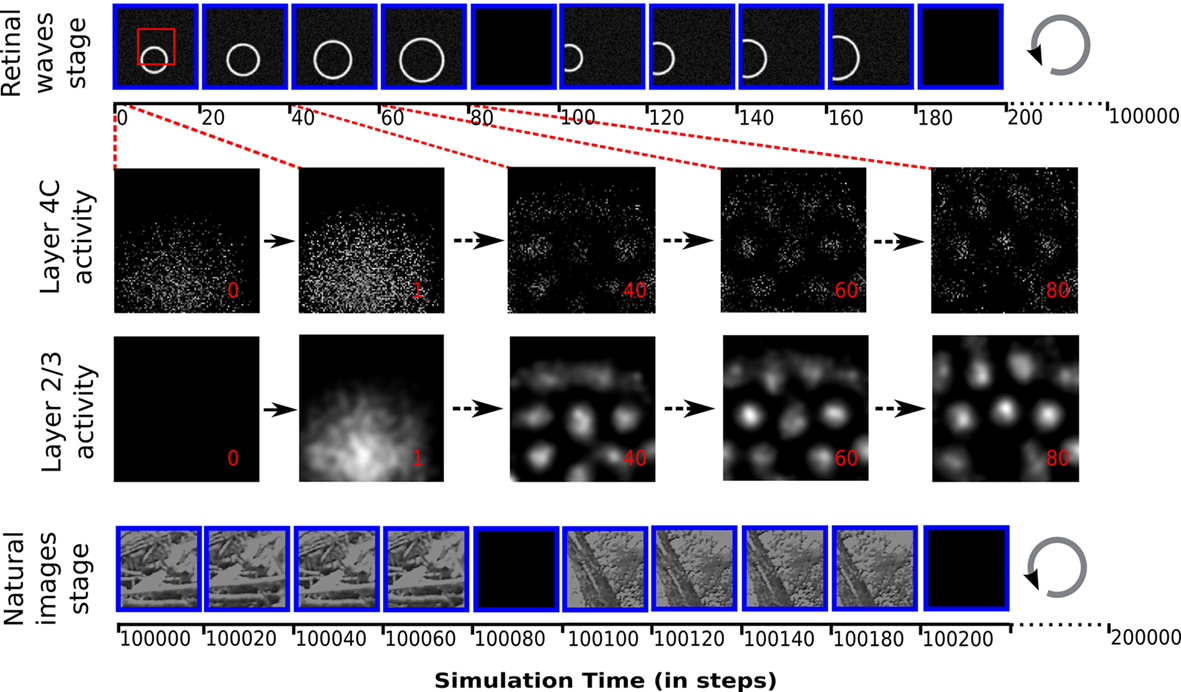
Figure 4. The protocol of input pattern presentation to the model, and the evolution of activity in the cortical sheets after presentation of a retinal wave to an untrained network. Each input pattern is presented 15 times (of which four are shown in the diagram for illustration), transformed (in the case of retinal waves, expanded, and in the case of natural images, translated in a random direction) relative to its initial position, followed by a blank stimulus. Each presentation lasts 20 time steps, during which the activity of the retinal sheet is kept constant. The input pattern presentation has two stages: 5000 iterations of expanding retinal waves, followed by 5000 iterations of natural images with randomly jittered positions. Over the 300 time steps that a given stimulus is presented, the layer 2/3 sheet activation gradually forms a pattern of blobs while the layer 4C sheet pattern has local disorder that persists only within the overall pattern of blobs matching the layer 2/3 sheet activity. These differences in activity patterns lead to different map organizations in layer 2/3 and 4C sheets, with layer 2/3 sheet developing smooth maps for orientation and phase (see Figure 6).The red rectangle outlines the region of the retinal sheet corresponding to the cortical 2/3 sheets.
Input patterns are presented to the model at each time step by activating the retinal photoreceptor units according to the gray-scale values in the chosen pattern or image. For each input pattern to be presented, a random initial position is set. Then this input pattern is presented 15 times for 20 time steps, each time expanded or translated by a small factor (see Figure 4). In the case of retinal waves the initial retinal wave is always expanded by a constant factor of 0.3 (in retinal sheet coordinates) per input presentation (see Figure 4 top panel). Natural images are always translated from the initial position in a random direction, over a distance chosen from a uniform random distribution between 0 and 0.4 (in retinal sheet coordinates; see Figure 4 bottom panel). This way the same input pattern is presented for 300 time steps of the simulation overall, with small differences in position. Each set of 15 presentations of the input pattern is followed by a single presentation of a constant zero stimulus to the retina (see Figure 4), which causes a decrease of activity in the network, and thus helps the network to form a different initial pattern of responses to the next stimulus. This blank input corresponds to the periods of silence between retinal waves during pre-natal development, and to the overall inhibition known to occur during saccades (Diamond et al., 2000) during post-natal development.
2.4 ON and OFF RGC/LGN Channels and Eye Opening
Because it is known that retinal waves activate both ON and OFF RGC cells at the same time (Kerschensteiner and Wong, 2008), in the first stage we bypass the processing that happens in the RGC/LGN sheets, as we cannot assume that activations in RGC/LGN ON and OFF sheets are anti-correlated before eye opening as they are in adult animals. Having correlated ON and OFF channels during pre-natal developmental in the model means that at the end of the first developmental stage, neurons in layer 4C have developed similar connection fields in both the ON and OFF channels. However, this means that after the normal RGC/LGN processing is enabled (corresponding to eye opening in an animal), neurons will lose their orientation selectivity, which would hinder the process of development of orientation maps. To see why orientation selectivity is lost, imagine a V1 neuron with a connection field twice as long vertically as it is horizontally, connecting equally to both ON and OFF LGN inputs. A vertical grating aligned with this connection field will activate about half of the incoming connections, either all from the ON or OFF channel. A horizontal grating will activate a similar number of connections, some from the light bars overlapping the ON connections and some from the dark bars overlapping the OFF LGN channels. Thus the response of the cell will be essentially unselective for orientation.
One way to ensure sufficient orientation selectivity of layer 4C neurons after eye opening is to assume that either the ON or the OFF RGC/LGN channel is stronger, which increases the response difference from aligned and orthogonal stimuli. Interestingly, experimental studies have shown that individual V1 neurons have highly variable ratio between the strength of ON and OFF RF subfields, and are on average biased toward the OFF channel (Jin et al., 2008; Yeh et al., 2009). Therefore in the model we randomize the ratio of the connection strength from the ON and OFF LGN sheets to layer 4C sheet neurons according to following formula:
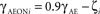
where γAE is the average strength of the LGN to layer 4C projection (see Table 1), ζ is a random variable drawn from uniform distribution from the interval [−0.5, 0.5], and γAEONi and γAEOFF are the resulting ON and OFF projection strength for neuron i. We found this randomization to be sufficient to preserve selectivity. Note that the overall results do not depend on this randomization; merely making the OFF channel uniformly stronger yields similar orientation maps and range of complexity values, but it results in an unrealistic bias toward OFF-center RFs.
2.5 Network Dynamics
Finally, let us briefly explain the dynamics that the above architecture imposes on the model, and how these dynamics ensure that the model can develop maps of complex cells. Let us assume the model is in the early stage of development, when neurons in layer 4C have only very weakly, if at all, orientation-selective RFs. Further, for the sake of simplicity, let us assume that previously the network has been presented with blank stimuli, ensuring that both cortical layers have zero activity.
Let us now present a new input to the network, such as a retinal wave. Given the unselective nature of RFs of layer 4C neurons at this stage and their high threshold, in the time step when the new input arrives from RGC/LGN to layer 4C many neurons will stay silent, however some will have elevated activities (see Figure 4). The population activity will be largely random (see Figure 4: activity at time 0). In the next time step, the activities from layer 4C arrive at layer 2/3, which will produce output generally following the activation pattern in layer 4C, but with a smoother profile due to the summation of afferent connection fields (see Figure 4: activity at time 1). Because of the relatively unspecific activation of L2/3 at this time point, the feedback pathway from layer 2/3 to layer 4C will not significantly shape the activity of layer 4C. However, because of the strong lateral interactions in L2/3, a few time steps later the activity in layer 2/3 will converge into a more selective activity profile with the “blobby” distribution typical for models with Mexican-hat-like lateral interactions (see Figure 4: activity at time 40). Similarly to the LISSOM model, during this period, the areas in L2/3 which are more activated relatively to their surrounding area via the feed-forward connections will gradually become more active, while the surrounding areas of neurons will become more and more inhibited, resulting in the typical blobby activity pattern (see Figure 4).
Once the blobby activity pattern is established, the feedback to layer 4C will have a very specific effect – the areas in layer 4C corresponding to activity blobs in layer 2/3 will be mildly excited, whereas the areas in layer 4C in the surround of activity blobs formed in layer 2/3 will be inhibited. The overall effect of these activations will be that neurons in layer 4C and layer 2/3 will be activated in the same areas, the difference being that in layer 2/3 the blobbs of activity are smooth due to the strong lateral interactions, whereas activity in layer 4C in the elevated areas will stay sparse because of the higher threshold of the neurons, jittered afferent connection fields, and lack of strong lateral contributions.
Let us now consider one specific blob of activity formed in L2/3, surrounded by unactivated neurons, and a corresponding spot of sparsely activated area in layer 4C, also surrounded by unactivated neurons. Each 20 time steps, Hebbian learning will ensure that the neurons in layer 4C that are activated will adapt to the current input pattern. Now let us consider presenting the same stimulus in the next step, but shifted slightly in spatial position. This means we can assume that the neurons in the area that we are discussing will typically see a stimulus with the same orientation but with a different phase. The dynamics in the network are not reset after each stimulus presentation, so when the new stimulus arrives at layer 4C, the layer will have generally the same activation profile as at the end of previous input presentation. However, because the new input is slightly different and because of the sources of variability in the model (the randomly shifted RFs of layer 4C neurons and the additive noise) it will activate a different subset of neurons within the discussed area. Note there will still be strong feedback from L2/3, which means that only neurons within the same area will be activated. The result is that at the end of settling, the same blob of neurons will be activated in L2/3 as in the previous step. Additionally, the same area of layer 4C will have elevated activities, but the subset of neurons activated will be different.
The dynamics of the model thus ensure that it maintains a stable activity profile in both cortical sheets over time, unless the input changes dramatically. Importantly, however, the activity profile in layer 4C is stable only at a large scale, whereas locally the network allows different subsets of neurons to be activated for subsequent input presentations. This property ensures that at large scale L4 will become organized in the same manner as L2/3, but locally it can capture the changes that occur over short time scales. If we assume the input is typically translated (either in one direction or in a random manner) over short periods of time, we can conclude that it should be this translation (e.g., change in phase) that will be locally captured by L4 neuron RFs. Overall, this process leads to map development in both layers 4C and 2/3, and at the same time to disordered phase representation in layer 4C. This explanation also underlines the importance of the difference between the strength of lateral activity in the two cortical layers – strong Mexican-hat-like activities in layer 4C would not allow nearby neurons to have significantly different activities, and consequently would not allow neurons with different phase preference to develop.
3 Results
3.1 Development of Maps of Complex Cells
In this section we present results from the model after pre-natal and post-natal development. All results shown are from the same simulation run for 200000 iterations, unless otherwise specified. The only components of the model that undergo adaptation during development are the afferent connections from RGC/LGN to layer 4Cβ, the lateral inhibitory connections in both cortical sheets, and the threshold of the layer 4Cβ neurons, so it is clear that any behavior that emerges during development is doing so as a result of these changes. One of the most important novel features of the model is that we assume strong lateral connections to be present in layer 2/3 and only weak ones in layer 4C. For the sake of clarity and simplicity, results presented in this section are from a model that completely lacks lateral connections in layer 4C, i.e., γLE = 0 and γLI = 0. The effects of layer 4C lateral connectivity are addressed in “Section 3.3.”
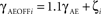
As can be seen in Figure 5, the projections from both the RGC/LGN On and the RGC/LGN Off sheets to layer 4Cβ developed oriented profiles, giving rise to orientation selectivity for units in layer 4Cβ. The lateral projections developed connections between regions with similar orientation preferences, as expected from physiological evidence (Bosking et al., 1997).
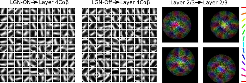
Figure 5. Sampling of final settled connection fields after 200000 input presentations. Only projections that are modified during development are shown: every 20th neuron in the projection from the ON RGC/LGN layer to layer 4Cβ (left), similarly for the projection from the OFF RGC/LGN layer to layer 4Cβ (middle), and sample lateral inhibitory projections in layer 2/3 (right). Each LGN ON weight pattern shows the pattern of LGN On-cell activity that would most excite V1 neuron, before engaging any lateral interactions in V1, and similarly for LGN Off. The color in the lateral inhibitory projection connection fields follows the color key on the right and indicates the orientation preference of the source neurons (see Figure 6), showing which L2/3 neurons will most inhibit this neuron.
One of the most important aspects of the model is its topographical organization. In order to assess the topographic properties we measured orientation and phase preference maps in both cortical sheets (Figure 6). We did this in a way analogous to the procedure used in optical imaging experiments (Blasdel, 1992). The network was presented with sinusoidal gratings of varying phase and orientation, and neuronal activity was recorded as these parameters of the stimulus were varied. The activity values were used to compute the orientation and phase preference of each unit by a vector averaging procedure (Miikkulainen et al., 2005).
Figure 6. Orientation selectivity maps, phase preference, and activity in the two cortical sheets of the model, at 40 and 200000 iterations. In the orientation selectivity and activity plots, each unit is color coded according to the orientation it prefers (as shown in the color key), and the saturation of the color indicates the level of orientation selectivity (how closely the input must match the unit’s preferred orientation for it to respond; unselective neurons appear white). Similarly, in the phase preference map each unit is color coded according to the phase it prefers (as shown in the color key, marked with degrees). The first two rows show these measures in the model before development, and the bottom two rows show the final measurement after the network was trained for 200000 iterations by presenting stimuli as described in Figure 4. The final layer 2/3 orientation maps are good match to experiments. Full experimental measurements are not available for any of the other plots.
As can be seen in Figure 6, layer 2/3 developed a smooth orientation map, containing the known signatures of cortical orientation maps (such as pinwheels, linear zones, saddle points, and fractures). Furthermore, at a coarser scale, orientation maps in layer 4Cβ match those in layer 2/3 (Figure 6). The orientation preference maps in layer 4Cβ contain some level of scatter, which although not previously reported, does not contradict any experimental evidence to the best of our knowledge. For instance, two-photon imaging studies (Ohki et al., 2005) have only shown that scatter is low for orientation preference in superficial layers such as layer 2/3, which is also the case in the model. The existence of some orientation preference scatter in cortical layer 4C is therefore one of the predictions of the model.
The second column of Figure 6 shows the phase preference of individual neurons. Phase preference is measured as the phase of the optimally oriented sine grating that evoked the maximal response of the neuron. This is a measurement of absolute phase, and depends both on the absolute position of the neuron’s RF in retinotopic coordinates and the position of the ON and OFF subfields within its RF. In the phase preference maps measured in layer 4C at 200000, one can see a very small level of clustering, but the overall appearance is much more disordered than that of the orientation preference map from the same layer. On the other hand, the phase preference maps formed in layer 2/3 of our model look radically different from those formed in layer 4C, with large iso-phase patches and overall smooth characteristics. It is important to note that the phase preference of units in layer 2/3, which (as we show below) behave like complex cells, is very weak. However, the existence of weak phase selectivity in complex cells is in line with experimental studies (Movshon et al., 1978; Ringach et al., 2002; Crowder et al., 2007). Currently we are not aware of any experimental study directly measuring the relationship between the (weak) phase preference of complex cells and their topography. The most common technique for measuring topographic maps in layer 2/3 in cortex – optical imaging – might simply not be sensitive enough to capture weak, though well-organized, phase preference maps within the population of complex cells. This result represents a second prediction that could in principle be tested in a detailed study of phase preferences in layer 2/3.
Finally, to assess whether the model cells behave like experimentally measured complex cells, we have calculated the MR index for all units. The MR index is a standard technique for classifying V1 neurons into simple and complex categories (Movshon et al., 1978). This value is computed as the F1/F0 ratio, where F1 is the first harmonic and F0 the mean of the response of the neuron to a drifting sinusoidal stimulus. The MR index classifies a neuron as complex if its value is below 1 and as simple if it is above 1. The histograms of the MR index of all cells in layers 4Cβ and 2/3 can be seen in Figure 7. As expected, according to the MR measure, the majority of neurons in layer 4C are classified as simple cells (96%), whereas most neurons in layer 2/3 are classified as complex cells (67%). When cells from layer 4Cβ and layer 2/3 are pooled together as in the Ringach study, one can observe the typical bimodal distribution (Figure 7). Note that the relative height of the two histogram peaks for the model data are arbitrary, as it depends on the number of neurons simulated in each layer; while the macaque data are pooled across multiple layers.
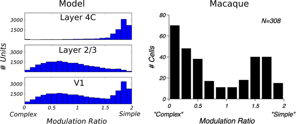
Figure 7. Comparison of the modulation ratio distribution in the model and in monkey V1. Data from the model (left), and data from Old World monkey reprinted from Ringach et al. (2002; right); both show a bimodal distribution.
One discrepancy between the experimental data and the model is the relative lack of model neurons with MRs close to zero (i.e., neurons that are almost perfectly insensitive to phase). Given the large number of free parameters in our model and the limited ability to fine tune them because of the high computational complexity of the model, it is possible that one could find a parameter combination that would make the model match the experimental results more closely in this respect. However, it is more likely that one will need to simulate a larger (higher density) version of the model to see a qualitative improvement in the number of low-MR neurons. In order to make the simulations practical, currently we set our model to have the lowest densities that still provide a reasonable match to experimental data. The actual density of neurons in cortex is several-fold higher in cat than in the implementation of the model. A higher density of neurons per model cortical area means that neurons in layer 2/3 pool information from larger number of neurons in layer 4Cβ, which makes it more likely that they will receive input from a wide range of phases, and consequently should lead to more neurons that are relatively insensitive to phase. Future increases in computational power or parallel implementation of the simulation software should allow such higher density models to be tested.
3.2 Single-Cell Properties
So far we have only discussed maps and population-level results. In order to compare the properties of the model to experimental data at the single-cell level, we measured orientation tuning curves and phase responses of example neurons in layer 4Cβ and layer 2/3 (Figure 8). This was done by presenting the model with orientation gratings of optimal spatial frequency, and varying phase and orientation while recording the activations of neurons; identical parameters of the RFs of all LGN filters in the model mean that the spatial frequency preference of the model neurons is virtually constant across the population. In order to save computational resources, we used this single known value of spatial frequency preference as the optimal spatial frequency for all neurons. The response of a neuron for a given orientation is defined as the strongest response of that neuron to sine gratings of the given orientation across all phases. The tuning curves are then constructed from the response at each orientation, for a given contrast.
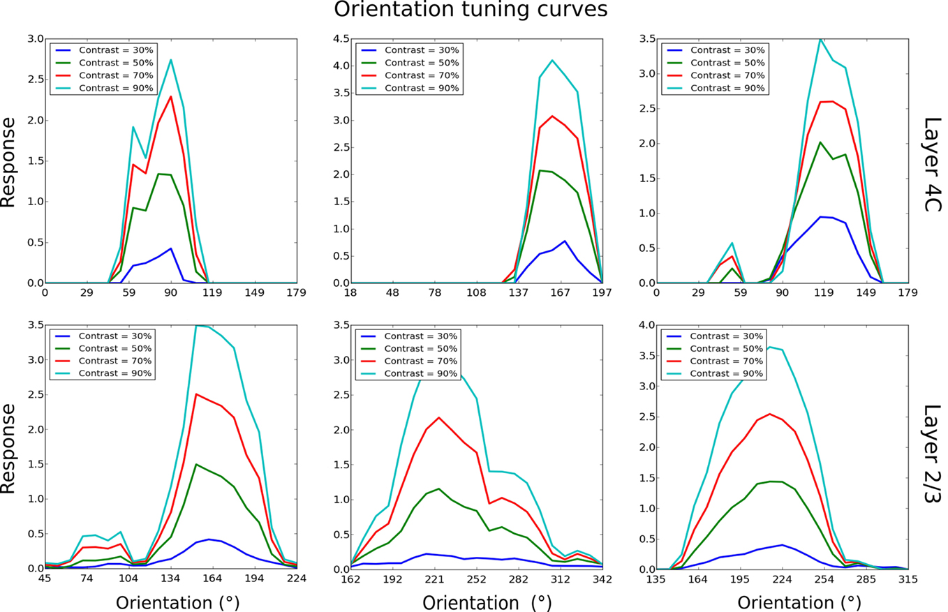
Figure 8. Orientation tuning curves of six example cells, three from layer 4Cβ and three from layer 2/3. As for these examples, most model neurons show contrast-invariant tuning. That is, the shape of the tuning curve is similar across a wide range of contrasts.
As illustrated in Figure 8, most neurons examined in layer 4C had narrow orientation tuning with realistically shaped tuning curves (Alitto and Usrey, 2004). Similarly, in layer 2/3, many neurons have sharp tuning, but some neurons have elevated responses to a wide range of orientations and are overall less well tuned. On average, neurons in layer 2/3 were more broadly tuned to orientation compared with neurons in layer 4Cβ, which follows observations from some experimental studies (Ringach et al., 2002). Furthermore, neurons in layer 4Cβ and the well-tuned neurons in layer 2/3 achieve contrast invariance of orientation tuning width (compare contrast = 30% with contrast = 90% in Figure 8), as expected for layer 2/3 cells (Sclar and Freeman, 1982).
Finally, we also show the responses of neurons with respect to the phase of an optimally oriented sinusoidal grating. As can be seen in Figure 9, the responses of layer 4Cβ cells, which develop high MRs, are very selective to phase, with zero response for most phases and a sharp peak around their preferred phase. In contrast to the selective response of simple cells, complex cells in the model generally show significantly elevated activity for most phases, as expected given their low-MRs (see Figure 7). Note that the complex cells do still show a clear preference for some phases, which underlies the weak phase preference maps that we observe in layer 2/3 in the model.
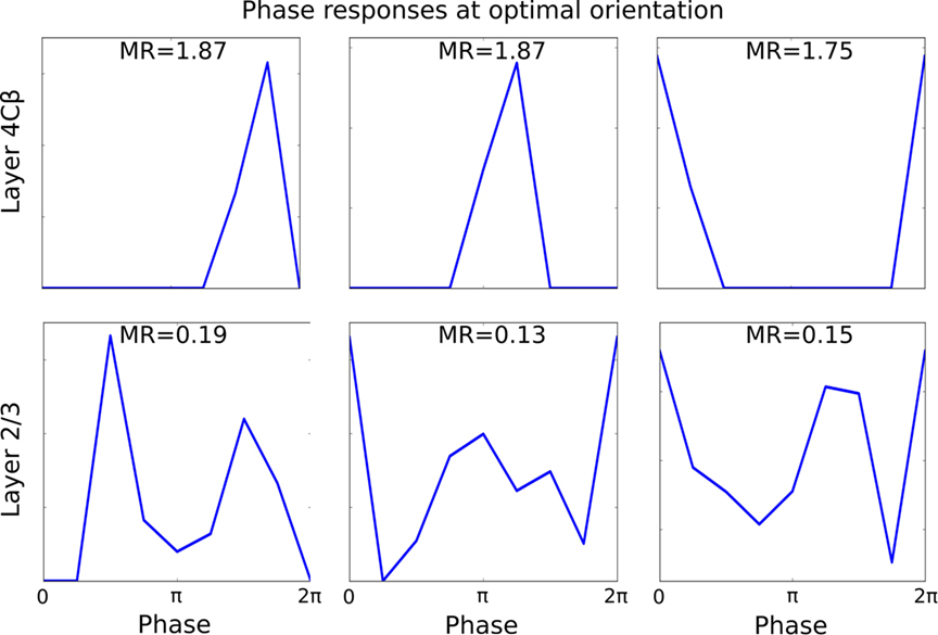
Figure 9. Responses of six representative cells, three from layer 4Cβ and three from layer 2/3, to the varying phase of an optimally oriented sine grating. Nearly all layer 4Cβ cells respond to only a small number of similar phases, while majority of layer 2/3 cells respond to all or nearly all phases.
3.3 Influence of Lateral Connections in Layer 4Cβ and Layer 2/3
One of the key differences of the model from previous models of development is moving strong lateral interactions from the simple-cell layer, to the complex-cell layer. Layer 4C, however, does contain lateral connections, albeit about 4 times less dense than layer 2/3 (based on cat data from Binzegger et al., 2009). In order to test the effect of lateral connections in layer 4C, we ran several simulations that extended layer 4C with both short-range excitatory and long-range inhibitory lateral connections identical to those in layer 2/3. We varied the ratio between the strength of the lateral interaction in layer 4C and layer 2/3 (henceforth called lateral interaction ratio, LIR) in order to examine the relative influence of these connections. Figure 10 shows that weak lateral connections in layer 4C do not significantly influence the results of the model, indicating the model is compatible with the known weaker lateral connectivity in layer 4C. However, with increasing strength of layer 4C lateral connections, one can observe increasing clustering of phases in layer 4C and consequently layer 2/3 neurons becoming more sensitive to phase. This result shows the importance of having weaker lateral interactions in the model layer 4C, as proposed.
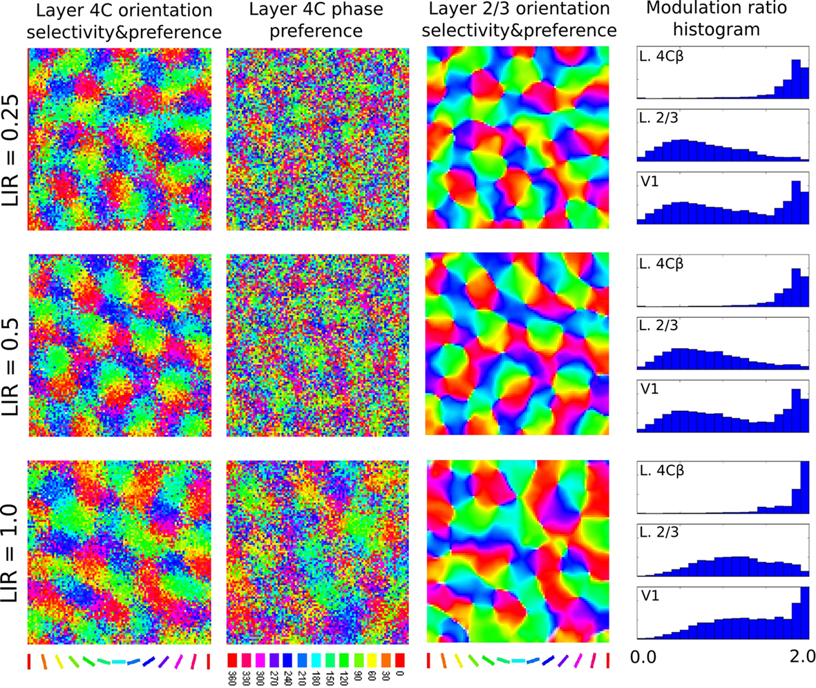
Figure 10. This figure demonstrates the influence of the strength of the lateral interaction in layer 4C relative to the strength of lateral interaction in layer 2/3 (the LIR index). Each row shows the results of a simulation run with a different LIR. The main properties of the model do not change if we add weak lateral connectivity to layer 4C, but adding strong lateral connectivity to layer 4C causes phase clustering in layer 4C, reducing phase invariance in layer 2/3 (notice how the MR histogram shifts in the “simple-cell” direction for L2/3 cells as LIR increases).
3.4 Relationship between Orientation Map Position and Modulation Ratio
Having a model of orientation map development with a wide distribution of MRs puts us in the unique position of being able to examine the relationship between these two features. In order to quantify the map position of a given neuron, we use the local homogeneity index (LHI) introduced by Nauhaus et al. (2008). This index approaches 1 as the local region of the map is occupied by more similar orientation preferences, and approaches 0 as the local region is occupied by diverse orientation preferences. Figure 11 shows that the model exhibits a noisy but clear trend of higher MRs in regions with low LHI and lower MRs in regions with high LHI, as confirmed by the weak but highly significant correlation (r = −0.228, p < 0.0001).
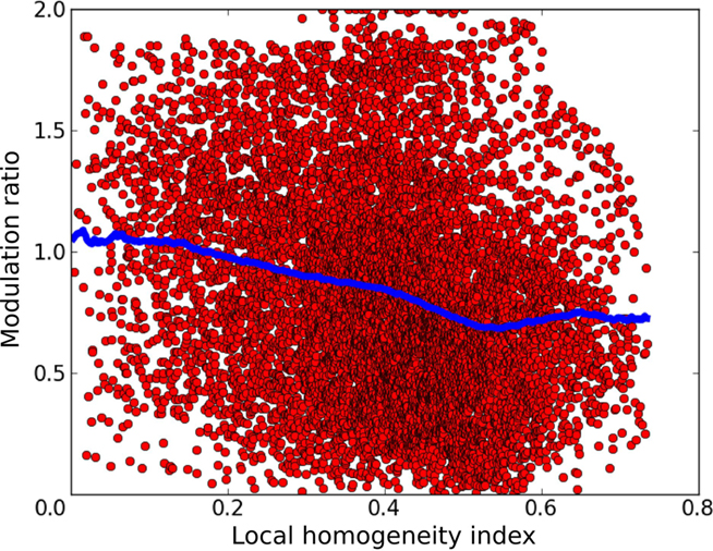
Figure 11. The relationship between the local homogeneity index and the modulation ratio. Each red point in this graph corresponds to a single neuron in layer 2/3 of the model. The x axis shows the LHI at the given neuron’s position and the y axis shows its modulation ratio. The blue dots show a sliding average of the distribution. A clear trend of decreasing modulation ratio with increasing LHI index is apparent, as confirmed by the weak but highly significant correlation (r = −0.228, p < 0.0001).
This indicates that model neurons in the center of orientation domains tend to have lower MRs than those located near singularities or fractures in the orientation map, a clear prediction for future experiments. This is because neurons in layer 2/3 near map discontinuities will receive connections from fewer neurons in layer 4C that have the same preferred orientation as many neurons at the same location in the map will be selective to other orientations. At the same time, this also means that such neuron will be pooling activities from more limited range of layer 4C neurons responding to its preferred orientation but selective to different phases, making it more likely that its response will be dominated by narrow range of phases. Thus neurons at singularities will be more likely to be selective to phase than neurons in the centers of orientation domains.
4 Discussion
The majority of models of functional map development use a Mexican-hat profile of lateral interactions as the main driving force for map development (Olson and Grossberg, 1998; Burger and Lang, 2001; Weber, 2001; Miikkulainen et al., 2005; Grabska-Barwinska and von der Malsburg, 2008). These lateral interactions ensure that throughout development, the activity in the network is strongly correlated at short ranges and is anti-correlated at medium ranges. Over time, these patterns of activation result in identical or very similar RFs developing among proximate neurons, whereas neurons at medium-ranges develop different RFs. This description of map development shows the conflict of such mechanisms with the apparent disordered phase representation in V1: cells with increasingly different phase preference should have increasingly anti-correlated activities, but Mexican-hat lateral connectivity leads to neurons in a local vicinity being correlated. Hence such models, in the absence of additional features, will develop a smooth phase representation, contrary to the experimental evidence.
Here we propose a model that provides a resolution to this conflict. The first key idea is to weaken the lateral interactions in the layer that is, after development, predominantly occupied by simple cells and receives direct thalamic input, and introduce them to the layer that is occupied by complex cells and does not receive direct thalamic input. This makes our two model cortical sheets a homolog of cortical layer 4C (which does receive the direct thalamic input and has weaker lateral connections) and layer 2/3 (which does not typically receive direct thalamic input, but rather its afferent input comes from layer 4, and has stronger lateral connections). The second essential ingredient of the model is the feedback connectivity from layer 2/3 to layer 4C, which ensures that matching maps can develop in both layers. This type of connectivity is supported experimentally, with evidence of a strong feedback pathway from layer 2/3 via layer 5 and 6 back to layer 4C (Alitto, 2003; Binzegger et al., 2004). Finally, we introduce several realistic sources of variability in the model, which ensure that the initial responses of neurons in layer 4C are sufficiently non-uniform. As the results from the simulations show (see Figure 6), these changes are sufficient to allow for disordered phase representation to develop in layer 4C. Once layer 4C has a disordered phase representation, complex cells are constructed very simply by pooling across a local area of simple cells.
The model cortical neurons develop elongated connection fields reminiscent of the Gabor-like RFs of V1 neurons. However, the population characteristics of the model RFs differ from animal RFs in two important features. First, nearly all of the model neurons are selective to roughly the same spatial frequency. Second, nearly all of the model RFs consist of either two or three ON or OFF lobes. In macaques, greater variability both in the spatial frequency preference and number of lobes is observed (Ringach, 2004). Both of these discrepancies can be linked to two related constraints introduced in our model for the sake of simplicity and computational efficiency – the single fixed frequency preference of all RGC/LGN neurons, and the fixed size of the afferent connection fields from the RGC/LGN to layer 4C neurons. Palmer (2009) has shown that closely related models with multiple RGC/LGN channels with different Difference-of-Gaussian RF sizes, along with corresponding differences in the afferent connection field sizes, develop not only a larger range of RF sizes and types, but also explain the development of maps of spatial frequency preference. In future work our model could be expanded to explain such variation and spatial frequency maps as well, as well as other response properties such as color, disparity, and motion preferences, at the cost of significantly greater complexity and computational requirements.
As we discussed before, there is experimental evidence that layer 4C contains predominantly simple cells, and that layer 2/3 contains predominantly complex cells. However, this difference is not as clear cut in macaque as in the model (Figure 7), and it has been proposed that simple and complex cells might not be separate populations but just part of a continuum (Mechler and Ringach, 2002; Priebe et al., 2004). In our model there is nothing fundamentally different between the cells that become simple or complex after development, other than the relative contributions of the different projections to individual neurons. For the sake of clarity and simplicity, in the model, the relative contributions of the different projections to a given neuron are fixed within each sheet, but different between the two sheets. If instead the ratio between the lateral and afferent connectivity was chosen independently for each neuron in each sheet, the MR index would vary as well, providing more complex-like cells in layer 4C and more simple-like cells in layer 2/3. Of course, this additional variability of projection strength would have to stay within the overall large-scale architecture proposed here, as this architecture is crucial for proper development of all the functional properties discussed here. Simulating this more complex version of the model could help clarify that the emergence of simple and complex response properties in the model is not due to a strict underlying dichotomy between two functional cell types, but rather a result of different balances between the different model projections in individual neurons and the different biases of these balances between layers.
Bearing in mind this potentially more complex circuitry due to randomness, one can see that our model contains elements of both of the two main previous hypotheses for how V1 circuitry leads to simple and complex cells. First, the model has a hierarchical feed-forward architecture reminiscent of Hubel and Wiesel’s (1962) original suggestion: that complex cells become phase invariant by pooling from simple-cells selective to the same orientation but a variety of phases. But the model also contains both lateral and interlaminar recurrent connectivity reminiscent of Chance et al.’s (1999) non-hierarchical model, which showed how phase-selective V1 cells could become phase invariant through local recurrent excitation. Importantly, both of these previous explanations require a local pool of simple-cells selective to the full range of phases, the major feature that this study was trying to reconcile with map development. The main difference between the previous models is how they sum from this local pool, whether directly (feed-forward model) or via other complex cells (recurrent model).
In our model, the hierarchical feed-forward architecture provides most of the phase invariance after development, due to pooling of simple-cell responses. But because there is some degree of clustering in the simple-cell phases, and because only a small number of simple cells provide direct input to the model complex cells, the individual complex-cell responses will not be completely phase invariant. Recurrent input from nearby complex cells can further smooth the responses and thus increase phase invariance, as in the Chance et al. (1999) model. Adding additional randomness in the relative strengths of afferent and lateral connectivity, as discussed above, would further blur the distinction between feed-forward or recurrent pooling. Moreover, the recurrent interactions in layer 2/3 drive the initial development of the maps, and are thus required for both simple and complex cells to emerge. Thus, our model relies on both of the main previous explanations for phase invariance, in order to provide a more complete account that also explains the development of these properties. The results demonstrate the importance of considering more comprehensive models that can place the principles from simple models in the context of more realistic connectivity while accounting for the process of development.
Our model and all previous models of complex-cell map development depend on a locally disordered representation of phase, allowing complex cells to achieve phase invariance by pooling from a local region of simple cells. As discussed in “Section 1,” the details of phase preference organization in V1 are controversial. Even so, all these studies show that spatial phase is much less organized than orientation, and one can thus expect to find a range of phases represented in a local region of V1. Furthermore, relatively limited clustering of phase in V1 will still lead to cells that have elevated activities in response to many phases of an optimally oriented sinusoidal grating, which in turn will ensure they are categorized as complex cells based on the F1/F0 ratio. On the other hand, even most complex cells will thus respond stronger to some phases – those over-represented in their local pool of simple cells – than to others, giving them a weak but measurable phase preference. Note that this result is consistent with the F0/F1 categorization, as only cells with 0 MR will have “perfectly invariant” response to phases (Ringach et al., 2002; Crowder et al., 2007).
In stark contrast to the highly disordered phase representation in layer 4C, the model predicts that nearby neurons in layer 2/3 will develop strongly correlated phase preference, again a phenomenon predicted by clustering of phase preference among simple cells and local activity pooling by complex cells. It will be interesting to see whether future two-photon imaging experiments or advances in optical imaging techniques will be able to confirm this predicted strong local correlation of (weak) phase preference among complex cells. Note that the predicted layer 4C and 2/3 organization differs markedly from the patterns predicted by Hyvärinen and Hoyer (2001) and Olson and Grossberg (1998) models. Due to the squaring of negative activities, the Hyvärinen and Hoyer (2001) model predicts perfectly random phase preference of simple cells, as suggested by their phase preference map. Even though Olson and Grossberg (1998) do not directly show the phase preference maps, it is reasonable to conclude their model will also not predict clustering of phase preference of simple cells, since it forces pairs of simple cells to develop opposite phases.
Although the basic operation of all the connections in the model is similar, only layer 4C afferent and layer 2/3 lateral connections show Hebbian plasticity, while others are kept fixed at their initial values. That is, the subcortical pathways, short-range excitatory, and the narrow afferent and feedback excitatory connectivity between layer 4C and 2/3 are all kept static. The afferent connections to layer 4C and the long-range connections are widely believed to be highly plastic during early development, as in the model. The subcortical pathways are kept constant with their adult pattern of organization, so that we can focus on the cortical development, but future work could consider subcortical plasticity as well. The remaining static connections are all short range, local connections within V1, either within each layer or between adjacent layers (4 and 2/3). A recent study by Buzás et al. (2006) found that the distribution of lateral connections with respect to orientation maps is best described by superposition of a spatially extended orientation-specific and a local orientation-invariant component, indicating that the short-range connectivity of pyramidal neurons in layer 2/3 is unselective. The functional specificity of the connections between layers 4C and 2/3 is currently unclear, however as they are also short range we have assumed that they are static as well. Should future experiments reveal specificity in any of the static projections, it is straightforward to make them plastic and study the effect this could have on development.
As described in “Section 2.2,” connection plasticity in the model is based on Hebbian learning with divisive normalization. Importantly, weights in the model are normalized jointly by type. That is, weights in afferent projections from the two LGN sheets are normalized together, while the long-range inhibitory connections are normalized in a separate pool, preserving a balance between feed-forward and recurrent processing and between excitatory and inhibitory projections. Separating these contributions to the neural response is crucial for ensuring that the model neurons develop robustly, retaining both afferent and lateral inputs and both excitation and inhibition. It is not known whether or how the different projections could be balanced in animal neurons, but several mechanisms are possible. For instance, inputs from these sources may arrive at different parts of the neuron, such as distal vs. proximal or basal vs. apical dendrites, which could each be regulated with some degree of independence that would correspond to the separate normalization in the model. Alternatively or in addition, connections may be regulated differently depending on chemical factors, either the different neurotransmitters involved [for GABAergic (inhibitory) vs. glutamatergic (excitatory) inputs] or because of neurotrophins specific to the given cell type providing the inputs. Such mechanisms have not yet been studied in detail, but it has been shown that, for instance, acetylcholine selectively controls the synaptic efficacy of feed-forward vs. intra-cortical synapses (Roberts et al., 2005). Determining the degree and mechanisms of projection-specific regulation of efficacy is an important topic for future experimental work.
An interesting characteristic of the model is that the formation of complex-cell-like RFs in layer 2/3 of the model assumes the existence of simple cells in layer 4Cβ. On the other hand, the strong lateral connectivity that is the driving force not only of the map but also of RF development is situated in layer 2/3, meaning the RF development of simple cells in layer 4Cβ is largely driven by feedback from complex cells in layer 2/3. To put it simply, the model uses a form of bootstrapping, where the development of complex cells requires the development of simple cells, and vice versa. The simulations show that with the correct parameterization, the dynamics of the model allow for such bootstrapping to work. In the model, sufficiently strong lateral interactions are required not only for orientation preference map formation, but also for the development of selective RFs. Because the model assumes only relatively weak lateral interaction in layer 4C, removing the feedback from layer 2/3 to layer 4C in the model prevents the neurons in layer 4C from developing oriented RFs, which in turn will prevent these properties appearing in layer 2/3. Therefore, the model predicts that the development of simple and complex cells cannot be decoupled and has to take place over the same time period for the observed properties of random phase in layer 4C, columnar orientation maps, and complex cells in layer 2/3 to develop.
Another interesting aspect of the model is the feedback connectivity from layer 2/3 to layer 4C. There are relatively few previous modeling studies looking either at feedback from higher-level areas to earlier visual areas (Schwabe et al., 2006) or the role of intra-areal feedback. The model shows that one role of the strong (albeit indirect) feedback pathway from layer 2/3 to layer 4C can be to ensure that similar selectivity for various features of the input (such as orientation) develops across the cortical layers. In future work, the model can provide insight into how the intra-areal feedback influences the properties of individual neurons in adult cortex, by measuring various properties of layer 4C neurons with feedback from layer 2/3 switched off.
As discussed in detail at the end of “Section 2.5,” the dynamics in the network ensure a relatively stable large scale “blobby” activity profile typical for the Mexican-hat-like lateral interactions in both layer 2/3 and 4C if the input pattern does not change dramatically, but at the same time, they allow layer 4C neurons to locally change activations in response to smaller changes in input. In layer 4C, these dynamics, together with Hebbian learning, can lead to development of maps with respect to the dominant features of the input at the larger scale, while at the local scale neurons can develop selectivities for range of features that tend to change at short time scale, even if these selectivities conflict with the Mexican-hat-like lateral interactions (i.e., nearby neurons can become selective to features that are not correlated in the input space). Due to the local pooling performed by the layer 2/3 neurons, this range of local selectivities can be transformed into responses that are invariant to features of the input that change at such short temporal scale. Because the layered architecture assumed by this model is present throughout the cortex, these same mechanisms could operate at many different levels of processing, forming maps, and invariances for various combinations of features depending on the input to the given cortical area. In particular, as we show here in the context of V1, this behavior allows neurons in layer 4C to respond to changes of phase as the input pattern is translated over short periods of time, and thus locally leads to development of cells selective to variety of phases in layer 4C and at the same time – on a larger scale – orientation maps develop in both cortical layers, with neurons in layer 2/3 becoming phase invariant.
Furthermore, one can see that in this way the model exploits the short-term temporal correlations to develop RFs invariant to the dominant fast changes in the input. It is thus possible to relate the model to learning algorithms such as slow feature analysis (Wiskott and Sejnowski, 2002) or the trace rule (Földiák, 1991). This shows that one can potentially substitute such elaborate single-neuron learning rules with an appropriate combination of dynamics in the network and a simple Hebbian learning rule, explaining how one can implement these advanced learning rules in a biologically plausible framework using simple constituents.
To the best of our knowledge, all previous developmental models of visual cortex that include lateral interactions place them in the layer containing simple cells. Although anatomical studies show that layer 4C contains lateral connections, they are significantly weaker (Binzegger et al., 2004; Chisum and Fitzpatrick, 2004; Hirsch and Martinez, 2006) and shorter (Rockland and Lund, 1983; Sincich and Blasdel, 2001; Binzegger et al., 2009) than those present in layer 2/3. Also, the lateral connectivity in layer 4C does not express the orientation-specific daisy pattern characteristic of the layer 2/3 lateral connections (Rockland and Lund, 1983; Sincich and Blasdel, 2001), which have been implicated in a number of functional properties of neurons in V1 such as orientation-selective surround modulation (Lamme, 1995; Jones et al., 2002). Although the previous models of cortical circuitry with strong lateral interactions between simple cells are not necessarily directly in conflict with experimental evidence, the experimental data highlight the need to explore models that consider layer 2/3 and complex cells as the main source of lateral interactions. In this respect, the model shows that it is possible to develop orientation maps in both layer 4C and layer 2/3 without any (or only weak) lateral connectivity within layer 4C. This result is largely due to feedback from layer 2/3 to layer 4C. Furthermore, neurons in layer 4C exhibit properties (for example the orientation-specific surround modulation) which are linked to the daisy-like pattern of lateral connections in layer 2/3 that is lacking in layer 4C. The proposed feedback mechanism could explain the missing link between these functional properties of layer 4C neurons and the anatomical features in layer 2/3 that are often believed to be responsible for them.
Another important advance from previous modeling studies of V1 map development is that the model has realistic single-cell responses in both simulated cortical layers, as demonstrated in Figure 8. Previous developmental studies have paid little attention to the more detailed properties of single cells such as the shape and sharpness of orientation tuning curves. In this model, individual simple and complex-cells develop realistic orientation tuning curves, arising from the interplay between the orientation-specific RF of each neuron with lateral interactions from neighboring neurons. Replicating these features is crucial for explaining how the neurons actually operate for visual inputs. Finally, in accordance with the experimental evidence, the model correctly predicts broader orientation tuning for complex cells than for simple cells. The fact that the model follows these additional constraints imposed by experimental studies, and that we have not intentionally sought them when designing the model, make us even more confident that the main new features of the model (the strong lateral connectivity in layer 2/3 with weak lateral connectivity in layer 4C, and feedback from layer 2/3 to layer 4C) reflect important aspects of the V1 architecture.
The large number of V1 properties that the model can demonstrate and the possibility to relate the model directly to anatomical properties of V1 comes at a cost. The model is complicated, both analytically and computationally, and contains a large number of free parameters. Where possible, we constrained these parameters to values known from experimental studies, but for most parameters the values of their biological counterparts are not known. These free parameters have been set through extensive empirical search, where the criterion was to find a model parametrization that follows all the constraints from experimental studies that we focus on in this study, i.e., variable phase preference development in layer 4C, complex-cell development in layer 2/3, and realistic orientation map shape. Due to the large number of free parameters and the high computational requirements of each simulation run (about 48 h on a modern CPU with 8 GB of memory), it is not possible to perform a rigorous parameter search to outline the region of parameter combinations in which we can achieve all the presented results.
The limited empirical parameter search that was possible to perform does suggest that there are some parameters to which the model is sensitive, particularly, the balance between the various projection strengths. It is unrealistic to assume each V1 neuron will have precisely balanced strength of connections from the different projections, but it is reasonable to assume this to be true on average for a local population of neurons. It is also likely that these and other free parameters of the model are actively regulated in animal V1 to achieve robust operation.
5 Conclusion
We have presented a comprehensive model of V1 function and development that depends only on know connectivity. The model develops smooth, matching, orientation preference maps in both cortical sheets. After development, layer 4C units become simple cells, with phase preference arranged randomly, while those in layer 2/3 are primarily complex cells. Both cell types express realistic contrast-invariant orientation tuning.
Our work diverges from the more common approach to build the simplest possible model that explains only a few properties of a system, and instead trades simplicity for the ability to explain a large number of properties in a single model. Because the brain is a significantly non-homogeneous and non-linear system, we believe such a modeling approach is inevitable, if we want to have a single consistent explanation for how the cortex works. At the same time, however, the approach highlights the importance of simple models, as it builds on top of the many insights obtained from them. Our work also shows that constructing such more complex models has the advantage of bringing insight into interactions between the various properties of V1, as demonstrated by the predictions we have formulated here. In particular, we predict limited but measurable clustering of the strong phase preferences in layer 4C, clear and smooth clustering of the weak phase preferences of complex cells in layer 2/3, and a tendency for neurons located at in-homogeneities in the orientation maps to have higher MRs.
Conflict of Interest Statement
The authors declare that the research was conducted in the absence of any commercial or financial relationships that could be construed as a potential conflict of interest.
Acknowledgments
Supported by the EPSRC/MRC Doctoral Training Centre in Neuroinformatics at the University of Edinburgh. Thanks to Judith Law, Chris Ball, and other members of the Institute for Adaptive and Neural Computation for helpful comments and discussion. This work has made use of computational resources provided by the Edinburgh Compute and Data Facility (ECDF). Thanks also to all of the Topographica developers, without whom this work would not have been possible.
References
Alitto, H. (2003). Corticothalamic feedback and sensory processing. Curr. Opin. Neurobiol. 13, 440–445.
Alitto, H. J., and Usrey, W. M. (2004). Influence of contrast on orientation and temporal frequency tuning in ferret primary visual cortex. J. Neurophysiol. 91, 2797–2808.
Aronov, D., Reich, D. S., Mechler, F., and Victor, J. D. (2003). Neural coding of spatial phase in V1 of the macaque monkey. J. Neurophysiol. 89, 3304–3327.
Bednar, J. A. (2009). Topographica: building and analyzing map-level simulations from Python, C/C++, MATLAB, NEST, or NEURON components. Front. Neuroinformatics 3:8. doi: 10.3389/neuro.11.008.2009
Bednar, J. A., Choe, Y., De Paula, J., Miikkulainen, R., Provost, J., and Tversky, T. (2004). Modeling cortical maps with Topographica. Neurocomputing 58–60, 1129–1135.
Binzegger, T., Douglas, R. J., and Martin, K. A. C. (2004). A quantitative map of the circuit of cat primary visual cortex. J. Neurosci. 24, 8441–8453.
Binzegger, T., Douglas, R. J., and Martin, K. A. C. (2009). Topology and dynamics of the canonical circuit of cat V1. Neural Netw. 22, 1071–1078.
Blakemore, C., and Price, D. J. (1987). The organization and post-natal development of area 18 of the cat’s visual cortex. J. Physiol. (Lond.) 384, 263–292.
Blasdel, G. G. (1992). Orientation selectivity, preference, and continuity in monkey striate cortex. J. Neurosci. 12, 3139–3161.
Bosking, W. H., Zhang, Y., Schofield, B., and Fitzpatrick, D. (1997). Orientation selectivity and the arrangement of horizontal connections in tree shrew striate cortex. J. Neurosci. 17, 2112–2127.
Burger, T., and Lang, E. W. (2001). Self-organization of local cortical circuits and cortical orientation maps: a nonlinear hebbian model of the visual cortex with adaptive lateral couplings. Z. Naturforsch. C 56, 464–478.
Buzás, P., Kovács, K., Ferecskó, A. S., Budd, J. M., Eysel, U. T., and Kisvárday, Z. F. (2006). Model-based analysis of excitatory lateral connections in the visual cortex. J. Comp. Neurol. 499, 861–881.
Buzás, P., Volgushev, M., Eysel, U., and Kisvárday, Z. (2003). Independence of visuotopic representation and orientation map in the visual cortex of the cat. Eur. J. Neurosci. 18, 957–968.
Chance, F. S., Nelson, S. B., and Abbott, L. F. (1999). Complex cells as cortically amplified simple cells. Nat. Neurosci. 2, 277–282.
Chapman, B., Stryker, M. P., and Bonhoeffer, T. (1996). Development of orientation preference maps in ferret primary visual cortex. J. Neurosci. 16, 6443–6453.
Chisum, H. J., and Fitzpatrick, D. (2004). The contribution of vertical and horizontal connections to the receptive field center and surround in V1. Neural Netw. 17, 681–693.
Crair, M., Gillespie, D., and Stryker, M. (1998). The role of visual experience in the development of columns in cat visual cortex. Science 279, 566–570.
Crowder, N. A., van Kleef, J., Dreher, B., and Ibbotson, M. R. (2007). Complex cells increase their phase sensitivity at low contrasts and following adaptation. J. Neurophysiol. 98, 1155–1166.
DeAngelis, G. C., Ghose, G. M., Ohzawa, I., and Freeman, R. D. (1999). Functional micro-organization of primary visual cortex: receptive field analysis of nearby neurons. J. Neurosci. 19, 4046–4064.
Diamond, M. R., Ross, J., and Morrone, M. C. (2000). Extraretinal control of saccadic suppression. J. Neurosci. 20, 3449–3455.
Einhäuser, W., Kayser, C., König, P., and Körding, K. P. (2002). Learning the invariance properties of complex cells from their responses to natural stimuli. Eur. J. Neurosci. 15, 475–486.
Grabska-Barwinska, A., and von der Malsburg, C. (2008). Establishment of a scaffold for orientation maps in primary visual cortex of higher mammals. J. Neurosci. 28, 249–257.
Hirsch, J. A., and Martinez, L. M. (2006). Laminar processing in the visual cortical column. Curr. Opin. Neurobiol. 16, 377–384.
Hubel, D. H., and Wiesel, T. N. (1962). Receptive fields, binocular interaction and functional architecture in the cat’s visual cortex. J. Physiol. 160, 106–154.
Hubel, D. H., and Wiesel, T. N. (1968). Receptive fields and functional architecture of monkey striate cortex. J. Physiol. (Lond.) 195, 215–243.
Hubel, D. H., and Wiesel, T. N. (1974). Sequence regularity and geometry of orientation columns in the monkey striate cortex. J. Comp. Neurol. 158, 267–294.
Hyvärinen, A., and Hoyer, P. O. (2001). A two-layer sparse coding model learns simple and complex cell receptive fields and topography from natural images. Vision Res. 41, 2413–2423.
Jin, J. Z., Weng, C., Yeh, C.-I. I., Gordon, J. A., Ruthazer, E. S., Stryker, M. P., Swadlow, H. A., and Alonso, J.-M. M. (2008). On and off domains of geniculate afferents in cat primary visual cortex. Nat. Neurosci. 11, 88–94.
Jones, H. E., Wang, W., and Sillito, A. M. (2002). Spatial organization and magnitude of orientation contrast interactions in primate V1. J. Neurophysiol. 88, 2796–2808.
Karklin, Y., and Lewicki, M. S. (2008). Emergence of complex cell properties by learning to generalize in natural scenes. Nature 457, 83–86.
Kayser, C., Einhäuser, W., and König, P. (2003). Temporal correlations of orientations in natural scenes. Neurocomputing 52–54, 117–123.
Kerschensteiner, D., and Wong, R. O. L. (2008). A precisely timed asynchronous pattern of on and off retinal ganglion cell activity during propagation of retinal waves. Neuron 58, 851–858.
Lamme, V. A. (1995). The neurophysiology of figure-ground segregation in primary visual cortex. J. Neurosci. 15, 1605–1615.
Law, J. S. (2009). Modeling the Development of Organization for Orientation Preference in Primary Visual Cortex. Ph.D. thesis, School of Informatics, The University of Edinburgh, Edinburgh.
Liu, Z., Gaska, J., Jacobson, L., and Pollen, D. (1z992). Interneuronal interaction between members of quadrature phase and anti-phase pairs in the cat’s visual cortex. Vision Res. 32, 1193–1198.
Martinez, L. M., and Alonso, J.-M. M. (2003). Complex receptive fields in primary visual cortex. Neuroscientist 9, 317–331.
Mechler, F., and Ringach, D. L. (2002). On the classification of simple and complex cells. Vision Res. 42, 1017–1033.
Miikkulainen, R., Bednar, J. A., Choe, Y., and Sirosh, J. (2005). Computational Maps in the Visual Cortex. Berlin: Springer.
Miller, K. (1994). A model for the development of simple cell receptive fields and the ordered arrangement of orientation columns through activity-dependent competition between ON- and OFF-center inputs. J. Neurosci. 14, 409–441.
Movshon, J. A., Thompson, I. D., and Tolhurst, D. J. (1978). Receptive field organization of complex cells in the cat’s striate cortex. J. Physiol. (Lond.) 283, 79–99.
Nagano, T., and Kurata, K. (1981). A self-organizing neural network model for the development of complex cells. Biol. Cybern. 40, 195–200.
Nauhaus, I., Benucci, A., Carandini, M., and Ringach, D. L. (2008). Neuronal selectivity and local map structure in visual cortex. Neuron 57, 673–679.
Ohki, K., Chung, S., Ch’ng, Y. H., Kara, P., and Reid, R. C. (2005). Functional imaging with cellular resolution reveals precise micro-architecture in visual cortex. Nature 433, 597–603.
Olson, S. J., and Grossberg, S. (1998). A neural network model for the development of simple and complex cell receptive fields within cortical maps of orientation and ocular dominance. Neural Netw. 11, 189–208.
Palmer, C. M. (2009). Topographic and Laminar Models for the Development and Organisation of Spatial Frequency and Orientation in V1. Ph.D. thesis, School of Informatics, The University of Edinburgh, Edinburgh.
Priebe, N. J., Mechler, F., Carandini, M., and Ferster, D. (2004). The contribution of spike threshold to the dichotomy of cortical simple and complex cells. Nat. Neurosci. 7, 1113–1122.
Ringach, D. L. (2004). Mapping receptive fields in primary visual cortex. J. Physiol. (Lond.) 558, 717–728.
Ringach, D. L. (2007). On the origin of the functional architecture of the cortex. PLoS ONE 2, 251. doi: 10.1371/journal.pone.0000251
Ringach, D. L., Shapley, R. M., and Hawken, M. J. (2002). Orientation selectivity in macaque V1: diversity and laminar dependence. J. Neurosci. 22, 5639–5651.
Roberts, M. J., Zinke, W., Guo, K., Robertson, R., McDonald, J. S., and Thiele, A. (2005). Acetylcholine dynamically controls spatial integration in marmoset primary visual cortex. J. Neurophysiol. 93, 2062–2072.
Rockland, K. S., and Lund, J. S. (1983). Intrinsic laminar lattice connections in primate visual cortex. J. Comp. Neurol. 216, 303–318.
Schwabe, L., Obermayer, K., Angelucci, A., and Bressloff, P. C. (2006). The role of feedback in shaping the extra-classical receptive field of cortical neurons: a recurrent network model. J. Neurosci. 26, 9117–9129.
Sclar, G., and Freeman, R. D. (1982). Orientation selectivity in the cat’s striate cortex is invariant with stimulus contrast. Exp. Brain Res. 46, 457–461.
Shouval, H., Goldberg, D., Jones, J., Beckerman, M., and Cooper, L. (2000). Structured long-range connections can provide a scaffold for orientation maps. J. Neurosci. 20, 1119–1128.
Sincich, L. C., and Blasdel, G. G. (2001). Oriented axon projections in primary visual cortex of the monkey. J. Neurosci. 21, 4416–4426.
Sullivan, T., and de Sa, V. (2004). A temporal trace and SOM-based model of complex cell development. Neurocomputing 58–60, 827–833.
von der Malsburg, C. (1973). Self-organization of orientation-sensitive cells in the striate cortex. Kybernetik 15, 85–100.
Warren, D., Fernandez, E., and Normann, R. (2001). High-resolution two-dimensional spatial mapping of cat striate cortex using a 100-microelectrode array. Neuroscience 105, 19–31.
Weber, C. (2001). “Self-organization of orientation maps, lateral connections, and dynamic receptive fields in the primary visual cortex,” in Proceedings of the International Conference on Artificial Neural Networks, Lecture Notes in Computer Science 2130 (Berlin: Springer), 1147–1152.
Willshaw, D. J., and von der Malsburg, C. (1976). How patterned neural connections can be set up by self-organization. Proc. R. Soc. Lond. B Biol. Sci. 194, 431–445.
Wiskott, L., and Sejnowski, T. J. (2002). Slow feature analysis: unsupervised learning of invariances. Neural Comput. 14, 715–770.
Keywords: topographic maps, simple cells, complex cells, development, cortex, visual, computational, model
Citation: Antolík J and Bednar JA (2011) Development of maps of simple and complex cells in the primary visual cortex. Front. Comput. Neurosci. 5:17. doi: 10.3389/fncom.2011.00017
Received: 20 January 2011;
Accepted: 30 March 2011;
Published online: 13 April 2011.
Edited by:
David Hansel, University of Paris, FranceReviewed by:
Jochen Triesch, Johann Wolfgang Goethe University, GermanyVirginia R. de Sa, University of California San Diego, USA
Copyright: © 2011 Antolík and Bednar. This is an open-access article subject to a non-exclusive license between the authors and Frontiers Media SA, which permits use, distribution and reproduction in other forums, provided the original authors and source are credited and other Frontiers conditions are complied with.
*Correspondence:Ján Antolík, Unité de Neurosciences Information et Complexité, CNRS UPR-3293, 1 Avenue de la Terrasse, 91198 Gif-sur-Yvette, France. e-mail: antolikjan@gmail.com