Short-term facilitation may stabilize parametric working memory trace
- 1 Department of Mathematics, University of Nebraska-Lincoln, Lincoln, NE, USA
- 2 Neurophysics and Physiology Laboratory, The Institute for Neurosciences and Cognition, Université René Descartes, Paris, France
- 3 Interdisciplinary Center for Neural Computation, The Hebrew University, Jerusalem, Israel
- 4 Department of Neurobiology, Weizmann Institute, Rehovot, Israel
- 5 Center for Theoretical Neuroscience, Columbia University, New York, NY, USA
Networks with continuous set of attractors are considered to be a paradigmatic model for parametric working memory (WM), but require fine tuning of connections and are thus structurally unstable. Here we analyzed the network with ring attractor, where connections are not perfectly tuned and the activity state therefore drifts in the absence of the stabilizing stimulus. We derive an analytical expression for the drift dynamics and conclude that the network cannot function as WM for a period of several seconds, a typical delay time in monkey memory experiments. We propose that short-term synaptic facilitation in recurrent connections significantly improves the robustness of the model by slowing down the drift of activity bump. Extending the calculation of the drift velocity to network with synaptic facilitation, we conclude that facilitation can slow down the drift by a large factor, rendering the network suitable as a model of WM.
Introduction
Working memory (WM) is an attentional function that enables the online holding and manipulation of information. WM is crucial to higher cognitive functions such as planning, reasoning, decision-making, and language comprehension (Baddeley, 1986; Fuster, 2008). The persistent activity recorded in specific groups of neurons in several cortical areas during WM tasks is thought to be the main neuronal correlate of WM (Fuster and Alexander, 1971; Miyashita and Chang, 1988; Funahashi et al., 1989, 1990; Romo et al., 1999, 2002). For example, a substantial fraction of neurons in the prefrontal cortex (PFC) elevate their activity selectively and persistently during the delay period of visuo-spatial WM tasks in which a monkey has to remember the direction of a visual cue for several seconds (Funahashi et al., 1989; Constantinidis and Steinmetz, 2001; Constantinidis and Wang, 2004).
This selective persistent activity must be created internally since during the delay period the sensory cue is absent. A classical view is that this activity reflects the existence of many intrinsic states of the PFC circuits, each of which is an attractor of the network dynamics (Hebb, 1949; Amit et al., 1997; Seung, 1998; Wang, 2001). Each state is characterized by a specific group of active neurons that sustain their activity through their recurrent interactions. In this framework, the transiently presented cue triggers the selection of a specific attractor in which network remains after the cue has disappeared until the behavioral task is performed (the delay period). Once the cue feature has lost its behavioral relevance the network returns to its baseline state. Therefore, during the delay, the neuronal activity encodes a memory trace of the cue feature.
The cue features that are kept in WM could be either of discrete nature (categorical), such as a visual object or a spoken word, or continuous, such as the frequency of a vibration or the spatial location of a visual stimulus. In the first case, a paradigmatic theoretical framework is a Hopfield-like network in which the dynamics display a discrete set of attractors (Hopfield, 1984; Amit, 1989). In the second case, on which the present paper focuses, the relevant framework is of a network with a continuous set of attractors.
To be specific we consider the case of visuo-spatial WM task. A model to account for the delay activity observed in these tasks is a recurrent network made of identical neurons with the geometry of a circle and a connectivity pattern such that the interaction strength between two neurons is fine-tuned to depend only on their distance on the ring (Amari, 1977). Therefore the network architecture is invariant to rotation. With sufficiently strong and spatially modulated recurrent excitation the network dynamics possess an infinite and continuous set (ring) of attractors (Ben-Yishai et al., 1995; Hansel and Sompolinsky, 1998). In an attractor the activity is persistent and its profile has the shape of a “bump” localized at an arbitrary location. A transient stimulus tuned to a specific location on the ring, corresponding to the direction to be memorized, selects the bump attractor which peaks at that location. After the stimulus is withdrawn, the network remains in this attractor (Figure 1). Therefore the network is able to encode in its activity the memory of the cue location.
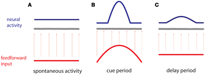
Figure 1. Working memory via persistent activity. A recurrent network of neurons (black circles) is ordered by a one-dimensional variable θ. (A) During spontaneous activity, the network receives a spatially homogeneous weak input (red), which results in a homogeneous profile of neural activity (blue). (B) During the cue period an inhomogeneous input (red), is received, peaked at a particular position θcue. The resulting profile of neural activity (blue) isa “bump” centered at the same position. (C) During the delay period the network receives a spatially homogeneous input, while the profile of neural activity remains inhomogeneous and centered at the same position.
While this mechanism is an attractive general proposal for a network basis of parametric WM, it suffers from an essential limitation. Indeed, it is structurally unstable: any deviation from the rotational symmetry, e.g., spatial heterogeneities in the connectivity or in intrinsic properties of the neurons, destroys the continuity of the attractor set (Tsodyks and Sejnowski, 1995; Zhang, 1996; Seung et al., 2000; Renart et al., 2003). In terms of WM, this means that during the delay period, the network state drifts toward an attractor that is only very weakly correlated with the cue position, leading to the loss of memory about the precise position of the cue.
Therefore the ring model can be a biologically realistic mechanism of parametric WM only if the recurrent connections are sufficiently fine-tuned to satisfy the following two conditions: (1) to guarantee the stability of the bump activity pattern and (2) to prevent its fast drift away from the cue position during the delay period. Moreover, the latter condition requires much tighter tuning than the former as indicated by previous analysis of this and other continuous attractor models (Tsodyks and Sejnowski, 1995; Zhang, 1996; Koulakov et al., 2002; Renart et al., 2003). Since there is little experimental evidence for the degree of tuning of neocortical connections, we address this issue theoretically by considering the ring model with strongly inhomogeneous connections that satisfy the first condition.
Connections between PFC pyramidal neurons exhibit increased level of short-term synaptic facilitation compared to primary sensory areas (Wang et al., 2006). Synaptic facilitation could be involved in WM by providing a memory trace lasting for up to several seconds (Mongillo et al., 2008). Here we show that short-term synaptic facilitation in recurrent interactions in PFC may be mitigating the inherent structural instability of the ring model by slowing down the degradation of the memory trace during the delay period. To this end we consider a rate model with “ring architecture” in which the symmetry of the network is broken due to random spatial fluctuations in the connectivity. We derive analytical one-dimensional approximations of the “bump” dynamics. This allows us to estimate the velocity of the drift of the activity bump and hence the rapidity at which the memory of the cue feature fades during the delay period. Subsequently, we argue that without facilitation, the drift is too fast and the number of attractors is too small for the memory trace to be accurate over the typical duration of the delay period used in WM experiments, which is of several seconds. However, synaptic facilitation temporarily modifies effective connection strengths, selectively amplifying connections between neurons that are activated by the cue. We demonstrate that this amplification tends to pin down the bump at its initial position. We show analytically that this slows down the drift dramatically (up to a factor of 100), so that no additional tuning of connections beyond that required for the stability of the bump is needed. We conclude that short-term facilitation may be essential to the stability of memory of continuous variables over delay duration up to a few tens of seconds.
Results
Working Memory Drift in the Presence of Synaptic Heterogeneity
The model
We consider a recurrent network which models a local circuit in dorsolateral PFC. It consists of a set of N units, or mini-columns, each of which corresponds to a group of PFC neurons with similar functional properties. The network has the architecture of a ring, a unit being labeled by its location θi on a circle (i = 1,..,N; −π≤θi<π). The population average firing rate of the i-th unit, denoted as mi = m(θi), satisfies the rate dynamics:
where [y]+ = max(0,y), and the synaptic matrix J is given by:

The first term in (2) depends only on the distance between the i-th and j-th units and therefore is invariant by translation along the ring. In the second term the elements nij are random and independently distributed with zero mean and unit variance. This represents random spatial fluctuations in the connection strengths between mini-columns and breaks the rotational symmetry on the ring. The two terms in (2) scale with the network size N so that each of their contributions to the total input  is finite (= O(1)) in the limit of large N. Note that the scaling N−1/2 of the heterogeneity term results in preservation of the “bump” attractor dynamics for ε = O(1) in the limit of large N (see next section).
The external input Ii(t) to the i-th mini-column, is the sum of two terms,  The background input Ib reflects the attentional state that we assume to depend on the epoch of the task. We take Ib ≤ 0 during pre-stimulus period whereas Ib = I0 > 0 during the delay period. The “cue” input
  is received during presentation of a transient sensory-related stimulus that is directionally selective (Figure 1).
Without synaptic heterogeneity (ε = 0), the interaction pattern is rotationally invariant and it is well-known (Ben-Yishai et al., 1995; Hansel and Sompolinsky, 1998; Blumenfeld et al., 2006) that if J1 > 1 (and for J0 sufficiently negative) the dynamics of the network in the presence of spatially homogeneous supra-threshold external input (i.e., Ii = I0 > 0), possess N stable attractors. At the attractor, the activity profile has the shape of a localized bump of activity given by

where ψ is the center of the bump and θc is its half-width that satisfies (see Appendix)
Upon presentation of the stimulus in direction θcue, during the cue period, the attractor with ψ = θcue is selected and the network remains in this state until the end of the delay period (Figures 1B,C). Therefore the cue direction is kept in the population activity of the network during the delay period.
Continuous attractor falls apart in the presence of synaptic heterogeneity
The continuity of the attractor set is broken in the presence of heterogeneities in the interactions, i.e., when ε ≠ 0 (Tsodyks and Sejnowski, 1995; Zhang, 1996; Seung et al., 2000; Renart et al., 2003). This happens even for arbitrary small ε. Although in this case the shape of the “bump” is very weakly perturbed by the interaction heterogeneities, there is only a small number of locations on the circle where it is stable. During the delay period the bump drifts to one of these locations as shown in the simulation results displayed in Figure 2A. As the interactions are more and more heterogeneous (increasing ε), the drift becomes even faster and the perturbation in the bumps shape becomes more severe, until it disappears completely. With the scaling of Eq. (2) this happens at ε that is on the order of one. Note that the Figure 2A used the value ε = 0.5; at this value the magnitude of the synaptic heterogeneities is significantly larger than the magnitude of the synaptic efficacies of the “unperturbed” Ring model (Figure A1 in Appendix). This is due to the different scalings w.r.t. N of these two terms in Eq. (2). Nevertheless, the approximate shape of the bump attractor was still roughly preserved.
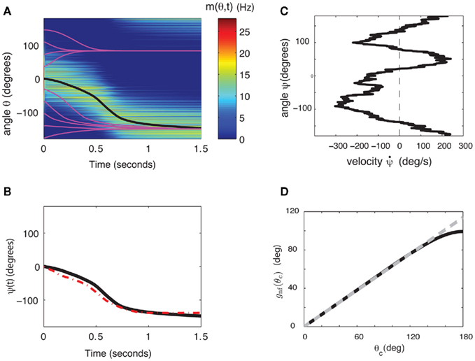
Figure 2. (A) Evolution of firing rates in a network with synaptic heterogeneity (ε = 0.5). Black curve indicates ψ(t) for the m(θ,t) plotted in color-scale. Magenta curves indicate ψ(t) for the solutions m(θ,t) with an initial bump centered at different angles. (B) Comparison of ψ(t), computed for the solution of the Ring model (black) and the reduced one-dimensional evolution according to Eq. (4) (red). (C) Plot of  as a function of ψ for the same instance of nij as in (A). Notice that two attractors from the (A) are at the angles where Fnf(ψ) is zero with negative slope. (D) The function gnf(θc) (black trace), that describes the dependence of the average speed on the bump width, is very well approximated by the linear function
  (gray line).
In order to gain a better understanding of the attractors of the dynamics and the robustness of the memory trace when the interactions are heterogeneous we derived an analytical approximation for the drift velocity under the assumption that N is large and that ε is small so that the shape of the bump is approximated by Eq. (3), i.e., m(θ,t) = m0(θ − ψ(t)) + O(ε), in the presence of constant spatially homogeneous input I0. A singular perturbation analysis of the dynamics (see Methods and also the Appendix) shows that the bump location ψ approximately follows the one-dimensional dynamics:
where m0(θ) is the “bump” profile (3) and θc is its half-width (see derivation in Appendix).
Although Eq. (4) was derived in the limit of small ε, it captures well the evolution of ψ(t) even if ε is relatively large. This is shown in the simulation results in Figures 2B,C (ε = 0.5). The fixed points of dynamics (4) are given by the solutions to the equation Fnf(ψ0) = 0. If the condition  is also satisfied, then this solution corresponds to a stable fixed point of (4), and therefore to the peak of a “bump” attractor of the dynamics (1). It should be noted that with our choice of the bump width (≈90°) there were typically two or three attractors of the dynamics of (1), and therefore these discrete attractors did not approximate the circle satisfactorily (Figure A2 in Appendix).
Equation (4) demonstrates that the dynamics of the firing rates in the ring model exhibit a structural instability, i.e., even a very small perturbation of the structure of the synaptic matrix causes a drift of the WM trace. However, this drift might not be a concern if it were happening on time-scales too slow to be relevant to the WM. For this reason we estimate the drifts average velocity.
Average drift velocity
The precise number of attractors and their location on the ring depend on the specific realization of the interaction pattern nij = n(θi,θj). For a given realization, the trajectory of the drift of the bump toward one of them depends also on its initial location at the beginning of the delay period. To get an estimate of the drift speed that is independent of the network realization we computed the square of the drift velocity averaged over the network realizations. Using Eq. (4) we found (see derivation in the Appendix) that

with  .
.
The mean square speed of the drift is thus inversely proportional to the square root of the number of mini-columns and to the time constant τ. It is also approximately proportional to the width of the bump (Figure 2D). Note that the mean square velocity  does not depend on the strength I0 of the background input because we have assumed a threshold linear input–output transfer function. For a more general transfer function the background input may affect the speed of the drift.
The size of a typical memory field measured in PFC (Funahashi et al., 1989, 1990) indicates that a possible range of values for the bump width θc is 60–100°. As for the timescale τ, its value in our simplified model should be taken as the typical time constants of the synapses in PFC (Shriki et al., 2003). Therefore if one assumes that interactions between PFC neurons is essentially mediated by AMPA and GABAA synapses, it is reasonable to take τ on the order of 5–10 ms. For the network size we take N = 720; this corresponds to a discretization of the representation of the cue feature with a precision of 0.5°. With these parameters and our choice1 of the heterogeneity strength ε = 0.5 Eq. (5) thus predicts a drift velocity on the order of many tens of degrees per second (with τ = 10 ms, the mean square velocity is in the range 71–119 deg/s for θc in the range of 60–100°). This is much larger than the drift velocity measured experimentally, which is on the order of 1–2 deg/s (White et al., 1994; Ploner et al., 1998). One would need to reduce ε by two orders of magnitude (e.g., ε = 0.005) to move the estimate (5) into the experimentally observed range. A drift velocity closer to, although still significantly faster than, experimental data can also be obtained if one assumes that in the PFC the synaptic time constants of the vast majority of the excitatory interactions are mediated by NMDA currents, with characteristic time constant in the range 50–100 ms.
Working Memory in the Presence of Short-Term Synaptic Facilitation
While bump attractor dynamics are preserved for values of the heterogeneity strength ε up to order O(1), the above analysis indicates that the drift of the activity bump may be too fast unless ε is chosen to be much closer to zero – i.e., unless the synaptic efficacies have much finer tuning than necessary for maintaining bump attractor dynamics. In the following we investigate an alternative mechanism which does not necessitate fine-tuned synapses, but instead relies on facilitation to slow down the drift.
Drift velocity of the “bump” slows down in the presence of synaptic facilitation
We assume now that the recurrent interactions display short-term plasticity properties that we model as in (Barak and Tsodyks, 2007; Mongillo et al., 2008). Therefore the dynamics of the network are given by
where two synaptic variables (u,x) describe the activity-dependent dynamics of synaptic efficacy: x stands for availability of synaptic resources and u stands for utilization factor, so that their product scales the synaptic strength. The variable u is up-regulated by presynaptic activity above its baseline value u = U (facilitation) and x is down-regulated by the activity below its baseline value x = 1 (depression). In the absence of firing, synaptic facilitation, and depression variables decay to their baseline levels with time constants tf and td respectively.
Simulations of these dynamics reveal that if the overall behavior of a single synapse is facilitating (e.g., U is small enough and tf ≫ td), the drift velocity of the bump is much slower for comparable shapes and heights of the bump (Figure 3B, cf. Figure 2A, see also Figure A3 in Appendix). To understand how this dramatic reduction in drift velocity results from synaptic facilitation we consider the limit in which the depression time constant is much faster than the facilitation time constant. We also assume that U is small, so that we can use a linear approximation for the dynamics of the facilitation variable u. In this limit, we can substitute x = 1 and approximate the dynamics of u by a linear equation, resulting in a system
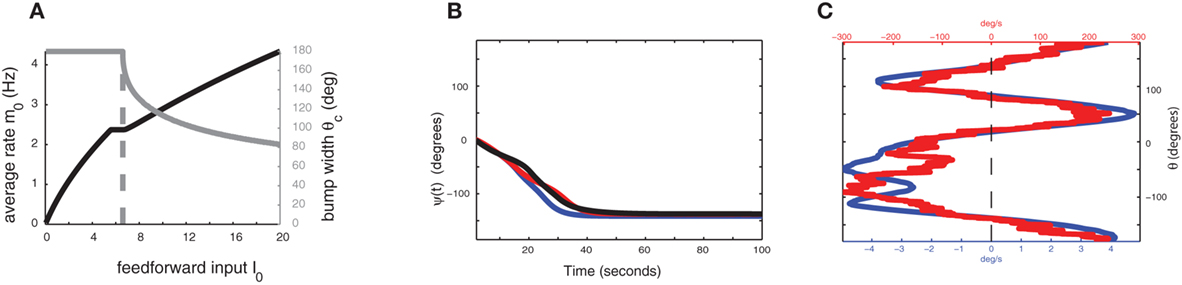
Figure 3. (A) The strength of external input I0 controls the width and stability of the bump attractor. Gray trace is the “bump” half-width θc, the black trace is the average firing rate m0. Dashed vertical line indicates the transition between stable spatially homogeneous solution (m = const) and the stable “bump” attractor. The synaptic parameters used here are the same as in Figure 3B. (B) Evolution of ψ(t) in the presence of synaptic facilitation; here the synaptic inhomogeneities nij are the same as in the simulation of Figure 2A. Black trace indicates ψ(t) for the full facilitation/depression model; blue trace indicates ψ(t) in the simplified facilitation model; red trace indicates ψ(t) in the one-dimensional reduction (8). (C) Comparison of profiles of ετ−1Fnf(ψ) (red) and εUFf(ψ) (blue).
In the absence of heterogeneities (ε = 0), the model with facilitation also exhibits a ring attractor in a certain range of synaptic parameters. However, unlike in the case of a network with constant synapses, transition from uniform state to ring attractor now depends on the strength of the supra-threshold external input I0 > 0, since recurrent connection effective strength increases with activity due to facilitation. In particular, for our choice of parameters, the uniform solution is stable for weak inputs, and activity bump appears for increasing input (Figure 3A). This scenario implies that if the baseline state of the network is below the transition, the considered circuit cannot keep the parametric memory trace, as a stable “bump” solution is needed for such a function. An additional external (non-specific) excitation, which could come, for example, from attentional regulation of the network, yields a ring of stable bump solutions and thus enables the circuit to perform its parametric WM function (Figure 1; note that both in the case with or without facilitation we assume that during the delay period there is a non-selective excitatory attentional signal).
As above, assuming that ε is small, we can derive an analytic expression for the evolution of ψ(t). One finds (see derivation in the Appendix) that

with
where 
 and the functions m0(θ) and u0(θ) are the attractors of the unperturbed (ε = 0) system (7). Equation (8) approximates well the dynamics of the center of the drifting bump (Figure 3B).
Attractors in the presence of synaptic facilitation
While the speed of the drift is significantly slowed in the presence of the synaptic facilitation, the attractors of the drift appear to be very similar in Figures 2A and 3B. In fact, the functions Ff(ψ) and Fnf(ψ), while on a different scale have very similar set of zeros (Figure 3C), and Ff(ψ) is close to “rescaling” of the function Fnf(ψ) (Figure A4 in Appendix).
It can be shown (see Appendix) that in the absence of facilitation the location of attractors of the Ring model does not depend on the strength of the feedforward input I0. This is no longer true in the presence of facilitation. In order to investigate how the location and the number of attractors are affected by the presence of synaptic facilitation we performed simulation in which we varied the strength of the constant feedforward input I0 fivefold. Figure 4B shows that although the function Ff(ψ) gained new attractors, these new attractors are not deep, i.e., small perturbations would easily let ψ(t) escape that attractor. The “deep” attractors, on the other hand, hardly change their location (see Figure 4A for the evolution of the attractors). This feature of the considered circuit ensures that the attractors during the delay period are not sensitive to realistic changes in input magnitude (such as ramping of rates from the previous layer). As the strength I0 of the feedforward input increases several-fold, the profile of Ff(ψ) eventually diverges from being close to a rescaled version of Fnf(ψ) (Figure A4 in Appendix).
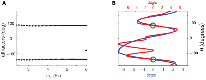
Figure 4. (A) Dependence of the attractors of the facilitated model on the average firing rate m0 as the strength of the feedforward input varies fivefold from I0 = 7 to I0 = 35. Dots represent attractors for the corresponding values of m0. (B) Comparison of  as a function of ψ for I0 = 7 (blue) and I0 = 35 (red). The deep attractors (circled brown) persist despite fivefold change of the amplitude of the feedforward input.
Synaptic facilitation slows down substantially the drift of the bump
How does the drift velocity depend on synaptic facilitation? To answer this question we have derived an analytical expression for the average of the mean square velocity of the drift. One finds that

with
See Appendix for the derivation and the explicit formulas for gf(θc, m0, tf).
In contrast to what we found in the absence of facilitation, the drift velocity depends on the spatial mean m0 of the “bump,” due to non-linear dependency of the synaptic input on the presynaptic activity. Note also that the time constant τ of the rate dynamics does not affect the drift velocity given by Eq. (9). This is because we have assumed here that this dynamics is much faster than the facilitation dynamics. This factor contributes substantially to the reduction in the velocity of the drift in presence of facilitation.
The ratio between the mean drift velocity without and with facilitation
is plotted in Figure 5 as a function of θc and m0 for values of U = 0.05, tf = 1 s, and τ = 10 ms. One sees that, facilitation may result in more than 100-fold slow down of the drift (Figure 5).
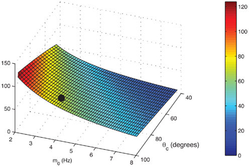
Figure 5. The ratio
 of mean square velocities without and with facilitation as a function of the bump width θc and the average firing rate m 0. The black dot indicates the same parameters (θc,m0) as in Figure 3B. Note that the average velocity of the drift is slower for lower m0 (and thus lower external input I0).
Discussion
Shortly after continuous attractors networks were proposed as a model of processing sensory stimuli with continuously varying features, the issue of structural instability of this model was identified (Tsodyks and Sejnowski, 1995; Zhang, 1996; Seung et al., 2000; Wang, 2001; Renart et al., 2003). In particular, when the network is not perfectly tuned, the continuous attractor is splitting into a small number of discrete attractors. This issue is especially relevant in case of WM networks, where information about the sensory cue is carried in the activity pattern of the network. In the case of ring model considered in this paper, the location of the activity bump encodes the stimulus feature and thus has to be stable on the time-scale of several seconds relevant for WM. The problem of structural stability is therefore of a quantitative nature – how long does it take for the bump to significantly drift away from its initial position determines the stability of the memory.
In this work, we considered a perturbation of the ring model obtained by adding a random component to the connectivity pattern that breaks its rotational invariance. We were then able to derive an analytic expression for the drift velocity of the bump under the condition that the perturbation is weak enough so that its shape is not significantly altered. This solution shows that, unless parameters are chosen such that synaptic efficacies are significantly more fine-tuned than what is necessary to preserve bump attractor dynamics, the bump may drift far away from the cue position very quickly, at a speed inconsistent with experimental observations. Whether such a precise tuning can be achieved biologically is an open question. It was addressed theoretically in (Renart et al., 2003) where ring model with inhomogeneities in neuronal thresholds was considered. The authors proposed a mechanism of synaptic tuning based on adiabatic plasticity, which significantly slowed down the drift velocity of the bump to realistic levels. We believe however that the ability of plastic cortical circuits to precisely tune themselves for one particular task can be limited due to constant bombardment by spiking inputs from other cortical areas that are not necessarily related to the particular WM task.
Motivated by recent experimental studies of synaptic connectivity in the PFC (Wang et al., 2006), we considered the effect of short-term synaptic facilitation on the ring model, and found that it significantly slows down the drift velocity, rendering the network suitable for WM. This solution eliminates the need for an additional fine tuning of the network connections. The reason facilitation makes the memory more stable is that when the activity bump is triggered by the input at a certain position, recurrent connections between the corresponding neurons facilitate and hence make it harder for the bump to drift away. This type of stability is complementary to the one demonstrated in (Mongillo et al., 2008), where it was shown that WM with facilitation is stable to brief suppression of spiking due to external perturbation.
In the present work, we have focused on the case where heterogeneities are in the connectivity pattern. However, our analysis can be extended to other sources of heterogeneities, e.g., in the intrinsic properties of the neurons or in the background inputs. For instance, in the latter case a similar approach as above shows that facilitation in the recurrent synaptic interactions can also slow down the drift velocity by roughly two orders of magnitude as it is the case when the heterogeneities are in the connectivity pattern (see Appendix.)
Our results have been derived in the framework of a single-population effective ring model (Amari, 1977; Ben-Yishai et al., 1995). In this framework excitatory and inhibitory neurons are lumped into one population of neurons and excitatory and inhibitory interactions are described by one effective interaction function with a “Mexican hat” profile. As a consequence, when facilitation is introduced it affects excitation as well as inhibition. However, our approach can be generalized straightforwardly to a two population rate models in which the four (EE, EI, IE, II) interactions are described separately. One can show that in this case, the drift velocity is also reduced considerably when the synapses of the excitatory neurons exhibit facilitation (Figure A5 in Appendix).
Finally, we would like to point out that in our analysis we assumed that rate dynamics is controlled by fast synaptic currents having the time-scale of several milliseconds, such as the case of AMPA-mediated glutamate current. At least some of the synaptic transmission between pyramidal cells in the PFC is mediated by NMDA receptors, which are much slower (τ ( 50–100 ms; see, e.g., Myme et al., 2003). Depending on the dominance of NMDA-mediated transmission, the bump stability will be slowed down proportionally to NMDA time constant, as can be seen, e.g., from Eq. (4) above. Whether PFC is characterized by increased prevalence of NMDA receptors compared to other cortical areas is controversial: while increased levels of mRNA for NMDARs were measured in a human postmortal immunohistological study (Scherzer et al., 1998), direct electrophysiological recordings found equal NMDA/AMPA current ratios in PFC and the visual cortex (Myme et al., 2003). What is the dominant mechanism for WM stabilization needs to be addressed in future experimental studies.
Methods
Neural Dynamics
We approximated the discrete system (1) by

While all analytic derivations (see Appendix) were performed using this continuous model and also system (7), all simulations were performed using the appropriate discrete models with N = 720 mini-columns. This corresponds to a spatial resolution of half a degree. Throughout the paper we used the following constants: the time-scale of the firing rate dynamics was assumed to be τ = 10 ms, while the time-scales of synaptic facilitation and depression were assumed to be tf = 1 s, and td = 0.1 s, cf (Barak and Tsodyks, 2007). We also assumed that the baseline level of the utilization of synaptic facilitation is U = 0.05; this corresponds to a maximal-possible 20-fold facilitation of an effective strength of a synapse. The magnitude of the synaptic heterogeneity used in the simulations was ε = 0.5.
Synaptic Parameters and Bump Attractors
We have used the following parameters for the model with facilitation and depression (6): J0 = −10, J1 = 8, I0 = 10. With these parameters, and the other constants defined as above, the unperturbed system has a stable family of bump attractors (3) with m0 ≈ 4.1 Hz, and θc ≈ 90°. We have chosen the parameters for the other two models, the simplified facilitation model (7) (J0 = −8.04, J1 = 3.48, I0 = 18.2) and for the ring model (1) (J0 = −10, J1 = 2.13, I0 = 40.4) so that they resulted in a stable bump attractor (3) of approximately the same width and height as in the model (6).
Scaling of the Synaptic Heterogeneity
We have chosen the scaling ε in Eq. (2) as ε = 0.5 for the model without facilitation. We have chosen the appropriate scaling εf in the other two models with facilitation so that  , where
  and
and  are the values used for the parameter J1 in Eq. (2) for the model with and without facilitation respectively. We chose this particular scaling in order to compensate for different values of J1 in different models. For example, if we assume that spatial fluctuations in the connectivity result from anatomical randomness in the number of connections between mini-columns, the amplitude of fluctuations will scale with the square root of the average number of connections, which in turn will be proportional to J1. We checked that choosing the fixed value of ε = 0.5 does not change the results significantly.
Evolution of the Bump Center
For a function q(θ,t) we denote its first Fourier coefficient as  and its phase as ψ(t). For models without facilitation, we used q = m to compute the center of bump ψ(t); for the model with facilitation and depression the effective synaptic input q(θ,t) = u(θ,t)x(θ,t)m(θ,t) was used; for the approximated model (7), q(θ,t) = u(θ,t)m(θ,t) was used. We used singular perturbation analysis to derive the evolution Eqs. (4) and (8) describing the dynamics of ψ(t); these derivations, as well as the derivations of mean square velocities are provided in Appendix.
Conflict of Interest Statement
The authors declare that the research was conducted in the absence of any commercial or financial relationships that could be construed as a potential conflict of interest.
Acknowledgments
Vladimir Itskov was partially supported by NSF DMS 0967377 and the Swartz Foundation, David Hansel was supported by ANR-09-SYS-002-01, and Misha Tsodyks by the Israeli Science Foundation. The work of David Hansel and Misha Tsodyks was also done in the framework of the France-Israel Lab. for Neuroscience (FILNe).
Footnotes
References
Amari, S. (1977). Dynamics of pattern formation in lateral-inhibition type neural fields. Biol. Cybern. 27, 77–87.
Amit, D. (1989). Modeling Brain Function: The World of Attractor Neural Networks. Cambridge, UK: Cambridge University press.
Amit, D. J., Fusi, S., and Yakovlev, V. (1997). Paradigmatic working memory (attractor) cell in it cortex. Neural Comput. 9, 1071–1092.
Barak, O., and Tsodyks, M. (2007). Persistent activity in neural networks with dynamic synapses. PLoS Comput. Biol. 3, e35.
Ben-Yishai, R., Bar-Or, R. L., and Sompolinsky, H. (1995). Theory of orientation tuning in visual cortex. Proc. Natl. Acad. Sci. U.S.A. 92, 3844–3848.
Blumenfeld, B., Bibitchkov, D., and Tsodyks, M. (2006). Neural network model of the primary visual cortex: from functional architecture to lateral connectivity and back. J. Comput. Neurosci. 20, 219–241.
Constantinidis, C., and Steinmetz, M. A. (2001). Neuronal responses in area 7a to multiple-stimulus displays: I. Neurons encode the location of the salient stimulus. Cereb. Cortex 11, 581–591.
Constantinidis, C., and Wang, X. J. (2004). A neural circuit basis for spatial working memory. Neuroscientist 10, 553–565.
Funahashi, S., Bruce, C. J., and Goldman-Rakic, P. S. (1989). Mnemonic coding of visual space in the monkey’s dorsolateral prefrontal cortex. J. Neurophysiol. 61, 331–349.
Funahashi, S., Bruce, C. J., and Goldman-Rakic, P. S. (1990). Visuospatial coding in primate prefrontal neurons revealed by oculomotor paradigms. J. Neurophysiol. 63, 814–831.
Fuster, J. M. (2008). The Prefrontal Cortex: Anatomy, Physiology, and Neuropsychology of the Frontal Lobe, 4th Edn. Philadelphia: Lippincott-Raven.
Fuster, J. M., and Alexander, G. E. (1971). Neuron activity related to short-term memory. Science 173, 652–654.
Hansel, D., and Sompolinsky, H. (1998). “Modeling feature selectivity in local cortical circuits,” In Methods in Neuronal Modeling. From Synapses to Networks, eds C. Koch, and I. Segev (Cambridge, MA: MIT Press), 499–567.
Hopfield, J. J. (1984). Neurons with graded response have collective computational properties like those of two-state neurons. Proc. Natl. Acad. Sci. U.S.A. 81, 3088–3092.
Koulakov, A. A., Raghavachari, S., Kepecs, A., and Lisman, J. E. (2002). Model for a robust neural integrator. Nat. Neurosci. 5, 775–782.
Miyashita, Y., and Chang, H. S. (1988). Neuronal correlate of pictorial short-term memory in the primate temporal cortex. Nature 331, 68–70.
Mongillo, G., Barak, O., and Tsodyks, M. (2008). Synaptic theory of working memory. Science 319, 1543–1546.
Myme, C. I., Sugino, K., Turrigiano, G. G., and Nelson, S. B. (2003). The nmda-to-ampa ratio at synapses onto layer 2/3 pyramidal neurons is conserved across prefrontal and visual cortices. J. Neurophysiol. 90, 771–779.
Ploner, C., Gaymard, B. M., Rivaud, S., Agid, Y., and Pierrot-Deseilligny, C. (1998). Temporal limits of spatial working memory in humans. Eur. J. Neurosci. 10, 794–797.
Renart, A., Song, P., and Wang, X. J. (2003). Robust spatial working memory through homeostatic synaptic scaling in heterogeneous cortical networks. Neuron 38, 473–485.
Romo, R., Brody, C. D., Hernandez, A., and Lemus, L. (1999). Neuronal correlates of parametric working memory in the prefrontal cortex. Nature 399, 470–473.
Romo, R., Hernandez, A., Zainos, A., Lemus, L., and Brody, C. D. (2002). Neuronal correlates of decision-making in secondary somatosensory cortex. Nat. Neurosci. 5, 1217–1225.
Scherzer, C. R., Landwehrmeyer, G. B., Kerner, J. A., Counihan, T. J., Kosinski, C. M., Standaert, D. G., Daggett, L. P., Velicelebi, G., Penney, J. B., and Young, A. B. (1998). Expression of N-methyl-D-aspartate receptor subunit mrnas in the human brain: hippocampus and cortex. J. Comp. Neurol. 390, 75–90.
Seung, H. S. (1998). “Learning continuous attractors in recurrent networks,” in Advances in Neural Information Processing Systems (Cambridge, MA: MIT Press), 654–660.
Seung, H. S., Lee, D. D., Reis, B. Y., and Tank, D. W. (2000). Stability of the memory of eye position in a recurrent network of conductance-based model neurons. Neuron 26, 259–271.
Shriki, O., Hansel, D., and Sompolinsky, H. (2003). Rate models for conductance-based cortical neuronal networks. Neural Comput. 15, 1809–1841.
Tsodyks, M., and Sejnowski, T. (1995). Associative memory and hippocampal place cells. Int. J. Neural Syst. 6, 81–86.
Wang, X. J. (2001). Synaptic reverberation underlying mnemonic persistent activity. Trends Neurosci. 24, 455–463.
Wang, Y., Markram, H., Goodman, P. H., Berger, T. K., Ma, J., and Goldman-Rakic, P. S. (2006). Heterogeneity in the pyramidal network of the medial prefrontal cortex. Nat. Neurosci. 9, 534–542.
White, J. M., Sparks, D. L., and Stanford, T. R. (1994). Saccades to remembered target locations: an analysis of systematic and variable errors. Vision Res. 34, 79–92.
Zhang, K. (1996). Representation of spatial orientation by the intrinsic dynamics of the head-direction cell ensemble: a theory. J. Neurosci. 16, 2112–2126.
Appendix
Computations for the Perturbed Ring Model without Facilitation
The non-perturbed ring model
We begin with some basic facts about the Ring model (Amari, 1977; Amit, 1989). Recall that the unperturbed (i.e., ε = 0) discretized Eq. (1) in the main text approximates its continuous analog

where [y]+ = max(0,y) denotes the threshold-linearity and  Denote

then it can be easily shown that

We model the delay period by assuming that during the delay period the feedforward input is constant: I(θ) = I0 = const. It is well-known that if J1 > 1 then there is a continuous family of steady states (“bumps”), centered at an arbitrary angle ψ:

where the bump’s half-width θc is related to the synaptic parameters via

while the Fourier coefficients m0 and m1 can be found from
Note that here the width of the bump depends only on J1, while the amplitude of the bump is proportional to I0 for large enough positive I0. It can be shown that for J1 < 1 the only fixed point is straight line (no bump solution), and that for J1 > 1 the only steady state is the “bump” – no stable straight–line solution. It particular, system (1) does not have a multi-stable regime with constant feedforward inputs (Amit, 1989).
The dynamics of ψ(t) in the presence of synaptic inhomogeneity
It follows from (2) that the time-dependent coefficients ψ(t) and m1(t) satisfy the following equations:
Motivated by Figure 2A, we would like to derive the dynamics of the perturbed Ring model with constant feedforward input:
where  As simulations suggest, during the delay period with constant feedforward input, the evolution of m(θ,t) can be described by

where m0(θ) is the steady state (3) centered at zero.
Using (5) and keeping in mind that (2) implies that  and also that
  we obtain the following:
Similarly, we obtain


Assuming the approximation of small ε we can see that the dynamics of m0, m1, and θc are on a faster timescale than the dynamics of ψ. Therefore, for the purpose of understanding the dynamics of ψ(t), we can approximate  where
where  is the first Fourier component of the bump attractor2 m0(θ) of the unperturbed (ε = 0) ring model with constant feedforward input I0. Taking into account the approximation m(θ,t) = m0(θ − ψ(t)) + O(ε) we obtain the following one-dimensional dynamics of ψ(t):

This in particular means that the attractors of the dynamics of ψ(t) do not depend on the scaling ε of the “noise” n(θ,θ′) as long as ε is small enough. These attractors can be found as the zeroes of Fnf(ψ) at which 
Computation of the mean square velocity without facilitation
Given a periodic function function n(θ,θ′) we define

Furthermore, we assume that the circle is discretized into N equal size bins with centers at θ1,…,θN, and that the values of n(θi,θj) is independently identically distributed, moreover  where nij are independent random variables with zero mean and unit variance. Note that the scaling of n(θi,θj) is chosen so that for large N and approximating the integrals by sums we obtain
in agreement with Eqs. (1) and (2) in the main text.
Lemma 1. Under the above assumptions and in the limit of large N, the following identity for the variance of Ff,g holds:

proof. Observe that
thus denoting fi = f(θi), gj = g(θj), and also using that 〈ni,jnk,l〉 = δikδij we obtain

this approximates the integral (12) in the limit of large N.□
Now we can use this computation with f(θ) = sinθ and g(θ) = m0(θ) to calculate the average square velocity (11) as

Note that the mean square velocity depends only on the half-width θc of the bump attractor m0(θ) and thus, thanks to identity (4), does not depend on I0, or J0. Moreover,  is well approximated by a linear function
  (see Figure 2F the main text) for most values of θc and is bounded by
Computations for the Simplified Facilitation Model
We use the following system, whose solutions approximate the solutions of the system with both facilitation and depression (Figure 3B in the main text)

where u(θ,t) is the facilitation variable, and U is the constant that determines the “depth” of facilitation (U = 0.05 in all simulations.) As before, we assume that 
We denote  and define the “location” ψ(t) of the “bump” as the phase of the first Fourier transform of q(θ,t):

Because the time constant of the rate dynamics (τ = 0.005 s throughout this paper) is much smaller than the time constant (tf = 1 s) of the dynamics of the facilitation variable u(θ), we can assume separation of time-scales, i.e., assume that the “fast” variable m(θ) is always near its attractor that is determined by the dynamics of the “slow” variable u. This implies that  and thus


where 
 and
and

Here

are the attractor3 of the unperturbed (ε = 0) system (13).
Using this and also the identity
we derive that
Similarly to the case of the drift with no-facilitation [see The Dynamics of ψ(t) in the Presence of Synaptic Inhomogeneity, (8)–(10)] it can be shown that the variables q0(t), q1(t), and θc(t) evolve on much faster time-scale than ψ(t). Since we are interested only in the dynamics of ψ(t), we therefore can consider the evolution of ψ(t) assuming that those variables are already near their respective attractors, i.e.,

Using (16), observing that  using the approximations (14) and also that m2 ≈ (m0(θ − ψ))2 + 2εm0(θ − ψ)η(θ,ψ) + O(ε2) we can discard the integrals of odd functions, we then derive
and thus obtain

where  and the functions q0(θ) = u0(θ)m0(θ) and m0(θ) are the attractors of the unperturbed (ε = 0) system (11).
Computation of the mean square velocity in the simplified facilitation model
Under the same assumptions as in Section “Computation of the Mean Square Velocity Without Facilitation” we can use Eq. (21) together with Lemma 1  to compute

where
While above formulae provide a method for computing the mean square velocity, what we really need to know is the dependence of the mean square velocity on the “observable” parameters m0 and θc. For this reason we need to find the dependence of the parameters J1, and  on those observables.
We consider the attractor m0(θ) and u0(θ) (13) of the unperturbed system (11) in the case of constant I(θ) = I0 = const. In this case J(θ, θ′) = J(θ − θ′) = 1/2π J0 + 1/π J1 cos(θ − θ′) and thus

where  ,
,  , and
, and  . These yield the following system of equations:
We observe from the first equation that  plug this into the second equation and then obtain
where

From here we obtain the following:
This furnishes the explicit relationship between J1,  on one hand and the observables m0 and θc on the other. Thus the formula (2.1) combined with

yields
where the function
can be computed from the following formulae:
Computations for the case of heterogeneities in the feedforward input and in the presence of simplified facilitation model
Here we derive the equations describing the dynamics for the drift of the neural activity when heterogeneities are present in the feedforward inputs (or alternatively in thresholds) I(θ). We consider the same model with synaptic facilitation:

where  is the unperturbed connectivity of the Ring model and ν(θ) is the heterogeneity in the feedforward inputs.
Similarly to Section “Computations for the Simplified Facilitation Model,” we denote  and define the “location” ψ(t) of the “bump” as the phase of the first Fourier transform of q(θ, t):
Because the time-constant of the rate dynamics (τ = 0.005 s throughout this paper) is assumed much smaller than the time-constant (tf = 1 s) of the dynamics of the facilitation variable u(θ, t), we can assume separation of time-scales, i.e., assume that the “fast” variable m(θ, t) is always near its attractor that is determined by the dynamics of the “slow” variable u This implies that  and thus

where  and
and  Differentiating the identity above we also obtain that

Using this and also the identity
we derive that
Similarly to the previous sections, it can be shown that the variables q0(t), q1(t), and θc(t) evolve on much faster time-scale than ψ(t). Since we are interested only in the dynamics of ψ(t), we therefore can consider the evolution of ψ(t) assuming that those variables are already near their respective attractors, i.e.,

Using this, Eq. (20), and also that

we can discard the integrals of odd functions of (θ − ψ(t)). We then derive

and thus obtain
where
Note that the function H(ψ) depends only on three parameters: the facilitation time-constant tf, the bump width  and the average firing rate
Computation of the mean square velocity for the case of heterogeneities in the feedforward input and in the presence of simplified facilitation model
Similarly to Lemma 1, it can be shown that if we assume that the circle is discretized into $N$ equal size bins with centers at  and the values of
  are independently identically distributed with zero mean and unit variance, then approximating the integrals by sums in the limit of large $N$ one obtains
where for any continuous function f(θ). Therefore, by taking  we obtain that
where the function
can be evaluated using Eqs. (17), (18), and (22).
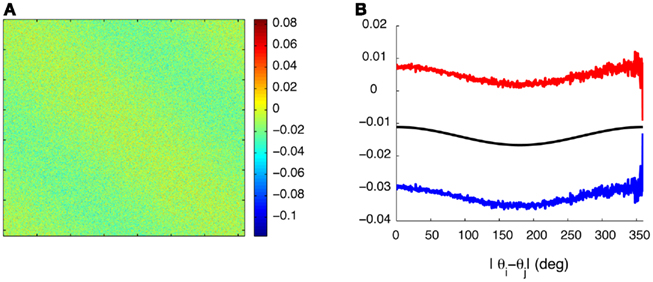
Figure A1. Synaptic heterogeneity may be significantly larger than the unperturbed Ring model synaptic efficacies, without destroying the bump-like attractors. (A) Colorplot of the synaptic matrix Jij Eq. (2) used in the Figure 1 of the main text. (B) The values of 1/N(J0 + 2J1cos(θi − θj)) (black trace) as a function of |θi − θj| versus that ±1 SD of the values Jij from [(A) red/blue traces] for each value of |θi − θj|.
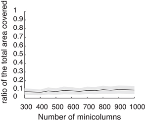
Figure A2. Discrete set of attractors of the Ring model with synaptic heterogeneity does not approximate a continuous attractor. Black trace indicates the average (over 200 trials) ratio of the total circle length covered by 3° intervals around each putative attractor. Gray area indicates 1 SD around the average. When the rotational invariance of the interactions is perturbed the set of discrete attractors does not provide a good approximation to a continuum ring attractor manifold even in the limit of large N. To show that we first found the points ψ0 on a circle that satisfy Fnf(ψ0) = 0 and  . These points are not guaranteed to be the exact actual centers of the bump attractors of the system (1), however every center of the attractor bump of (1) is in an O(ε) – neighborhood of one such point. We therefore overestimate the actual number of attractors. The mean number of putative attractors slowly grows, with increasing N, although for a realistic number of mini-columns it is rather low. However, it is not the number of attractors per se that makes it possible to approximate the continuous attractor by a collection of discrete attractors: it is rather the distribution of how the attractors are placed on the circle that matters. To quantify the proportion of the entire circle covered by putative attractors, we draw an interval around each of them (3° in our simulations) to determine the percentage of the total area covered. Numerical study revealed that their coverage either does not grow or grows slowly for the range of tested N; it only reaches up to 9.9% for N = 1000.
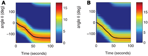
Figure A3. (A) Evolution of m(θ, t) in the full facilitation-depression model with the same matrix of heterogeneities nij as in Figure 2A. Black curve indicates ψ(t). For the first 3 s (brown bar at the bottom) the network is presented with the feedforward cue input, while after the cue the network is presented with constant feedforward input. (B) Evolution of m(θ,t) according to the simplified model with facilitation with the same matrix nij as in (A) and Figure 2A. Black curve indicates ψ(t). For the first 3 s (brown bar at the bottom) the network is presented with the feedforward cue input, while after the cue the network is presented with constant feedforward input.
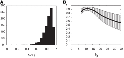
Figure A4. Similarity of Fnf(ψ) and Ff(ψ
). We have used the cosine of the angle
as a measure of similarity between the functions Fnf(ψ) and Ff(ψ). Note that − 1 ≤ cosγ ≤ 1. The value cosγ = 1 implies that Ff(ψ) = constFnf(ψ). (A) Histogram of cosine angles for I0 = 10. For each instance (Ntrials = 1000) of the synaptic heterogeneity nij the value of cosγ was computed. For comparison, Figure 3C had cosγ ≃ 0.936. (B) Same angles as in panel (A) were computed now as a function of the strength I0 (5 ≤ I0 ≤ 35). Mean of cosγ is the black trace, while the error bars mark 1 SD.
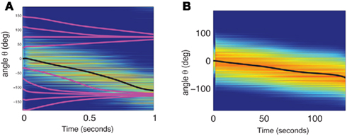
Figure A5. (A) The dynamics of two neuronal populations was simulated (see below). The activity of the excitatory population is shown in exactly the same manner as in Figure 2A of the main text. The evolution of firing rates  of N = 720 excitatory and firing rates
  of N = 720 inhibitory neurons was modeled using the rate model
where τE = 10 ms, τI = 5 ms, 
 and the synaptic strengths of the (global) projections of the excitatory neurons are

with a1 = 0.5, a2 = 5, ε = 0.5. The matrices  and
and  were drawn independently from normal distribution with zero mean and unit variance. (B) The dynamics of two neuronal populations where the excitatory synapses exhibit facilitation and depression. Similarly to the one-population model, the velocity of the drift is slowed down by at least two orders of magnitude. The evolution of firing rates was modeled as
where a1 = 1, a2 = 10,  ,
,  and the other parameters were chosen as described above or the Section “Methods.”
Keywords: parametric working memory, continuous attractors, synaptic facilitation, Ring model, bump attractor, working memory, inhomogeneous neural media, neural fields
Citation: Itskov V, Hansel D and Tsodyks M (2011) Short-term facilitation may stabilize parametric working memory trace. Front. Comput. Neurosci. 5:40. doi: 10.3389/fncom.2011.00040
Received: 22 January 2011; Paper pending published: 17 March 2011;
Accepted: 08 September 2011; Published online: 24 October 2011.
Edited by:
Stefano Fusi, Columbia University, USAReviewed by:
Albert Compte, Institut d ′Investigacions Biomèdiques August Pi i Sunyer, SpainCopyright: © 2011 Itskov, Hansel and Tsodyks. This is an open-access article subject to a non-exclusive license between the authors and Frontiers Media SA, which permits use, distribution and reproduction in other forums, provided the original authors and source are credited and other Frontiers conditions are complied with.
*Correspondence: Vladimir Itskov, Department of Mathematics, University of Nebraska-Lincoln, 244 Avery Hall, Lincoln, NE 68588, USA. e-mail: vitskov2@math.unl.edu