1
INRIA, Sophia-Antipolis, France
2
INLN, Valbonne, France
3
Université de Nice, Nice, France
We present a mathematical analysis of networks with integrate-and-fire (IF) neurons with conductance based synapses. Taking into account the realistic fact that the spike time is only known within some finite precision, we propose a model where spikes are effective at times multiple of a characteristic time scale δ, where δ can be arbitrary small (in particular, well beyond the numerical precision). We make a complete mathematical characterization of the model-dynamics and obtain the following results. The asymptotic dynamics is composed by finitely many stable periodic orbits, whose number and period can be arbitrary large and can diverge in a region of the synaptic weights space, traditionally called the “edge of chaos”, a notion mathematically well defined in the present paper. Furthermore, except at the edge of chaos, there is a one-to-one correspondence between the membrane potential trajectories and the raster plot. This shows that the neural code is entirely “in the spikes” in this case. As a key tool, we introduce an order parameter, easy to compute numerically, and closely related to a natural notion of entropy, providing a relevant characterization of the computational capabilities of the network. This allows us to compare the computational capabilities of leaky and IF models and conductance based models. The present study considers networks with constant input, and without time-dependent plasticity, but the framework has been designed for both extensions.
Neuronal networks have the capacity to treat incoming information, performing complex computational tasks (see Rieke et al., 1996
for a deep review), including sensory-motor tasks. It is a crucial challenge to understand how this information is encoded and transformed. However, when considering in vivo neuronal networks, information treatment proceeds usually from the interaction of many different functional units having different structures and roles, and interacting in a complex way. As a result, many time and space scales are involved. Also, in vivo neuronal systems are not isolated objects and have strong interactions with the external world, that hinder the study of a specific mechanism (Frégnac, 2004
). In vitro preparations are less subject to these restrictions, but it is still difficult to design specific neuronal structure in order to investigate the role of such systems regarding information treatment (Koch and Segev, 1998
). In this context models are often proposed, sufficiently close from neuronal networks to keep essential biological features, but also sufficiently simplified to achieve a characterization of their dynamics, the most often numerically and, when possible, analytically (Gerstner and Kistler, 2002b
; Dayan and Abbott, 2001
). This is always a delicate compromise. At one extreme, one reproduces all known features of ionic channels, neurons, synapses… and lose the hope to have any (mathematics and even numeric) control on what is going on. At the other extreme, over-simplified models can lose important biological features. Moreover, sharp simplifications may reveal exotic properties which are in fact induced by the model itself, but do not exist in the real system. This is a crucial aspect in theoretical neuroscience, where one must not forget that models are subject to hypothesis and have therefore intrinsic limits.
For example, it is widely believed that one of the major advantages of the integrate-and-fire (IF) model is its conceptual simplicity and analytical tractability that can be used to explore some general principles of neurodynamics and coding. However, though the first IF model was introduced in 1907 by Lapicque (1907) and though many important analytical and rigorous results have been published, there are essential parts missing in the state of the art in theory concerning the dynamics of IF neurons (see e.g., Ernst et al., 1995
; Gong and van Leeuwen, 2007
; Jahnke et al., 2008
; Memmesheimer and Timme, 2006
; Mirollo and Strogatz, 1990
; Senn and Urbanczik, 2001
; Timme et al., 2002 and references below for analytically solvable network models of spiking neurons). Moreover, while the analysis of an isolated neuron submitted to constant inputs is straightforward, the action of a periodic current on a neuron reveals already an astonishing complexity and the mathematical analysis requires elaborated methods from dynamical systems theory (Coombes, 1999b
; Coombes and Bressloff, 1999
; Keener et al., 1981
). In the same way, the computation of the spike train probability distribution resulting from the action of a Brownian noise on an IF neuron is not a completely straightforward exercise (Brunel and Latham, 2003
; Brunel and Sergi, 1998
; Gerstner and Kistler, 2002a
; Knight, 1972
; Touboul and Faugeras, 2007
) and may require rather elaborated mathematics. At the level of networks the situation is even worse, and the techniques used for the analysis of a single neuron are not easily extensible to the network case. For example, Bressloff and Coombes (2000b)
have extended the analysis in Coombes (1999b)
, Coombes and Bressloff (1999) and Keener et al. (1981)
to the dynamics of strongly coupled spiking neurons, but restricted to networks with specific architectures and under restrictive assumptions on the firing times. Chow and Kopell (2000)
studied IF neurons coupled with gap junctions but the analysis for large networks assumes constant synaptic weights. Brunel and Hakim (1999)
extended the Fokker–Planck analysis combined to a mean-field approach to the case of a network with inhibitory synaptic couplings but under the assumptions that all synaptic weights are equal. However, synaptic weight variability plays a crucial role in the dynamics, as revealed, e.g., using mean-field methods or numerical simulations (Van Vreeswijk, 2004
; Van Vreeswijk and Hansel, 1997
; Van Vreeswijk and Sompolinsky, 1998
). Mean-field methods allow the analysis of networks with random synaptic weights (Amari, 1972
; Cessac, 1995
; Cessac et al., 1994
; Hansel and Mato, 2003
; Samuelides and Cessac, 2007
; Sompolinsky et al., 1988
; Soula et al., 2006
) but they require a “thermodynamic limit” where the number of neurons tends to infinity and finite-size corrections are rather difficult to obtain. Moreover, the rigorous derivation of the mean-field equations, that requires large-deviations techniques (BenArous and Guionnet, 1995
), has not been yet done for the case of IF networks with continuous time dynamics (for the discrete time case, see Samuelides and Cessac, 2007
; Soula et al., 2006
).
Therefore, the “analytical tractability” of IF models is far from being evident. In the same way, the “conceptual simplicity” hides real difficulties which are mainly due to the following reasons. IF models introduce a discontinuity in the dynamics whenever a neuron crosses a threshold: this discontinuity, that mimics a “spike”, maps instantaneously the membrane potential from the threshold value to a reset value. The conjunction of continuous time dynamics and instantaneous reset leads to real conceptual and mathematical difficulties. For example, an IF neuron without refractory period (many authors have considered this situation), can, depending on parameters such as synaptic weights, fire uncountably many spikes within a finite time interval, leading to events which are not measurable (in the sense of probability theory). This prevents the use of standard methods in probability theory and notations such as  (spike response function) simply lose their meaning
[1
. Note also that the information theory (e.g., the Shannon theorem, stating that the sampling period must be less than half the period corresponding to the highest signal frequency) is not applicable with unbounded frequencies. But IF models have an unbounded frequencies spectrum (corresponding to instantaneous reset). From the information theoretic point of view, it is a temptation to relate this spurious property to the erroneous fact that the neuronal network information is not bounded. These few examples illustrate that one should not be abused by the apparent simplicity of IF models and must be careful in pushing too much their validity in order to explore some general principles of neurodynamics and coding.
(spike response function) simply lose their meaning
[1
. Note also that the information theory (e.g., the Shannon theorem, stating that the sampling period must be less than half the period corresponding to the highest signal frequency) is not applicable with unbounded frequencies. But IF models have an unbounded frequencies spectrum (corresponding to instantaneous reset). From the information theoretic point of view, it is a temptation to relate this spurious property to the erroneous fact that the neuronal network information is not bounded. These few examples illustrate that one should not be abused by the apparent simplicity of IF models and must be careful in pushing too much their validity in order to explore some general principles of neurodynamics and coding.The situation is not necessarily better when considering numerical implementations of IF neurons. Indeed, it is known from a long time that the way the membrane potential is reset in a neuronal network simulation have significant consequences for the dynamics of the model. In particular, Hansel et al. (1998)
showed that a naive implementation of IF dynamics on a discrete time grid introduces spurious effects and proposed an heuristic method to reduce the errors induced by time discretization. In parallel, many people have developed event based integration schemes (Brette et al., 2007
), using the fact that the time of spike of a neuron receiving instantaneous spikes from other neurons can be computed analytically, thus reducing consequently the computation time and affording the simulation of very large networks. In addition, exact event based computational schemes are typically used for the above-mentioned analytically tractable model classes (see, e.g., Mirollo and Strogatz, 1990
; Timme et al., 2002
). Unfortunately, this approach suffers two handicaps. If one considers more elaborated models than analytically tractable models, one is rapidly faced to the difficulty of finding an analytical expression for the next spike time (Rudolph and Destexhe, 2006
). Moreover, any numerical implementations of a neural network model will necessarily introduce errors compared to the exact solution. The question is: how does this error behave when iterating the dynamics? Is it amplified or damped? In IF models, as set previously, these errors are due to the discontinuity in the membrane potential reset and to the time discretization. This has been nicely discussed by Hansel et al. (1998)
. These authors point out two important effects. When a neuron fires a spike between time t and t + Δt a local error on the firing time is made when using time discretization. First, this leads to an error on the membrane potential and second this error is propagated to the other neurons via the synaptic interaction term. Unfortunately, this analysis, based on numerical simulations, was restricted to a specific architecture (identical excitatory neurons) and therefore the conclusions drawn by the authors cannot be extended as it is to arbitrary neural architectures. Indeed, as we show in the present paper, the small error induced by time discretization can be amplified or damped, depending on the synaptic weights value. This leads to the necessity of considering carefully (that is mathematically) the spurious effects induced by continuous time and instantaneous reset in IF models, as well as the effects of time discretization. This is one aspect discussed in the present paper.
More generally, this work contains several conclusions forming a logical chain. After a discussion on the characteristic times involved in real neurons and comparison to the assumptions used in IF models we argue that discrete time IF models with synchronous dynamics can be used to model real neurons as well, provided that the time scale discretization is sufficiently small. More precisely, we claim that IF equations are inappropriate if one sticks to much on the instantaneous reset and spike time, but that they provide a good and mathematically tractable model if one allows reset and spike to have some duration. We therefore modify the reset and spike definition (while keeping the differential equation for the dynamics of the membrane potential below the threshold). The goal is however NOT to propose yet another numerical scheme for the numerical integration of continuous time IF models. Instead, our aim is to analyze mathematically the main properties of the corresponding dynamical system, describing the evolution of a network with an arbitrary, finite, size (i.e., we do not use neither a mean-field approach nor a thermodynamic limit). We also consider an arbitrary architecture. Finally, in our analysis the time discretization step is arbitrary small (thus possibly well below the numerical precision). For this, we use a dynamical system approach developed formerly in Blanchard et al. (2000) and Cessac et al. (2004)
. In particular, in Cessac (2008)
a discrete time version of a leaky IF network, was studied. It was shown that the dynamics is generically periodic, but the periods can become arbitrary large (in particular, they can be larger than any accessible computational time) and in (non generic) regions of the synaptic weights space, dynamics is chaotic. In fact, a complete classification of the dynamical regimes exhibited by this class of IF models was proposed and a one-to-one correspondence between membrane potential trajectories and raster plots was exhibited (for recent contributions that study periodic orbits in large networks of IF neurons, see Gong and van Leeuwen, 2007
; Jahnke et al., 2008
). Beyond these mathematical results, this work warns one about some conclusions drawn from numerical simulations and emphasizes the necessity to have, when possible, a rigorous analysis of the dynamics.
The paper (Cessac, 2008
) dealt however with a rather simple version of IF neurons (leaky IF) and one may wonder whether this analysis extend to models closer to biology. In the present paper we extend these results, and give a mathematical treatment of the dynamics of spikes generated in synaptic coupled IF networks where synaptic currents are modeled in a biophysically plausible way (conductance based synapses). As developed in the text, this extension is far from being straightforward and requires a careful definition of dynamics incorporating the integration on the spikes arising in the past. This requires a relatively technical construction but this provides a setting where a rigorous classification of dynamics arising in IF neural networks with conductance based synapse can be made, with possible further extension to more elaborated models.
The paper is organized as follows. In Section 1 we give a short presentation of continuous time IF models. Then, a careful discussion about the natural time scales involved in biological neurons dynamics and how continuous time IF models violate these conditions is presented. From this discussion we propose the related discrete time model. Section 2 makes the mathematical analysis of the model and mathematical results characterizing its dynamics are presented. Moreover, we introduce an order parameter, called d(Ω,  ), which measures how close to the threshold are neurons during their evolution. Dynamics is periodic whenever d(Ω, ) is positive, but the typical orbit period can diverge when it tends to 0. This parameter is therefore related to an effective entropy within a finite time horizon, and to the neural network capability of producing distinct spikes trains. In other words, this is a way to measure the ability of the system to emulate different input–output functions. See Bertschinger and Natschläger (2004) and Langton (1990)
for a discussion on the link between the system dynamics and its related computational complexity
[2
. The smaller d(Ω, ), the larger is the set of distinct spikes trains that the neural network is able to produce. This implies in particular a larger variability in the responses to stimuli. The vanishing of d(Ω, ) corresponds to a region in the parameters space, called “the edge of chaos”, and defined here in mathematically precise way. In Section 3 we perform numerical investigations of d(Ω, ) in different models from leaky IF to conductance based models. These simulations suggest that there is a wide region of synaptic conductances where conductance based models display a large effective entropy, while this region is thinner for leaky IF models. This provides a quantitative way to measuring how conductances based synapses and currents enhances the information capacity of IF models. Section 4 proposes a discussion on these results.
), which measures how close to the threshold are neurons during their evolution. Dynamics is periodic whenever d(Ω, ) is positive, but the typical orbit period can diverge when it tends to 0. This parameter is therefore related to an effective entropy within a finite time horizon, and to the neural network capability of producing distinct spikes trains. In other words, this is a way to measure the ability of the system to emulate different input–output functions. See Bertschinger and Natschläger (2004) and Langton (1990)
for a discussion on the link between the system dynamics and its related computational complexity
[2
. The smaller d(Ω, ), the larger is the set of distinct spikes trains that the neural network is able to produce. This implies in particular a larger variability in the responses to stimuli. The vanishing of d(Ω, ) corresponds to a region in the parameters space, called “the edge of chaos”, and defined here in mathematically precise way. In Section 3 we perform numerical investigations of d(Ω, ) in different models from leaky IF to conductance based models. These simulations suggest that there is a wide region of synaptic conductances where conductance based models display a large effective entropy, while this region is thinner for leaky IF models. This provides a quantitative way to measuring how conductances based synapses and currents enhances the information capacity of IF models. Section 4 proposes a discussion on these results.General Structure of Integrate and Fire Models
We consider the (deterministic) evolution of a set of N neurons. Call Vk(t) the membrane potential of neuron k ∈{1 … N} at time t and let V(t) be the vector  . We denote by V ≡ V(0) the initial condition and the (forward) trajectory of V by:
. We denote by V ≡ V(0) the initial condition and the (forward) trajectory of V by:
where time can be either continuous or discrete. In the examples considered here the membrane potential of all neurons is uniformly bounded, from above and below, by some values Vmin, Vmax. Call  = [Vmin, Vmax]N. This is the phase space of our dynamical system.
= [Vmin, Vmax]N. This is the phase space of our dynamical system.We are focusing here on “IF models”, which always incorporate two regimes. For the clarity of the subsequent developments we briefly review these regimes (in a reverse order).
The “fire” regime
Fix a real number θ ∈[Vmin, Vmax] called the firing threshold of the neuron
[3
. Define the firing times of neuron k, for the trajectory
[4
V, by:

where  . The firing of neuron k corresponds to the following procedure. If Vk(t) ≥ θ then neuron membrane potential is reset instantaneously to some constant reset value Vreset and a spike is emitted toward post-synaptic neurons. In mathematical terms firing reads
[5
:
. The firing of neuron k corresponds to the following procedure. If Vk(t) ≥ θ then neuron membrane potential is reset instantaneously to some constant reset value Vreset and a spike is emitted toward post-synaptic neurons. In mathematical terms firing reads
[5
:
. The firing of neuron k corresponds to the following procedure. If Vk(t) ≥ θ then neuron membrane potential is reset instantaneously to some constant reset value Vreset and a spike is emitted toward post-synaptic neurons. In mathematical terms firing reads
[5
:
where Vreset ∈[Vmin, Vmax] is called the “reset potential”. In the sequel we assume, without loss of generality, that Vreset = 0. This reset has a dramatic effect. Changing the initial values of the membrane potential, one may expect some variability in the evolution. Now, fix a neuron k and assume that there is a time t > 0 and an interval [a, b] such that, ∀Vk(0) ∈[a, b], Vk(t) ≥ θ. Then, after reset, this interval is mapped to the point Vreset. Then, all trajectories born from [a, b] collapse on the same point and have obviously the same further evolution. Moreover, after reset, the membrane potential evolution does not depend on its past value. This induces an interesting property used in all the IF models that we know (see e.g., Gerstner and Kistler, 2002b
). The dynamical evolution is essentially determined by the firing times of the neurons, instead of their membrane potential value.
The “Integrate regime”
Below the threshold, Vk < 0, neuron k’s dynamics is driven by an equation of form:

where C is the membrane capacity of neuron k. Without loss of generality we normalize the quantities and fix C = 1. In its most general form, the neuron k’s membrane conductance gk > 0 depends on Vk [see e.g., Hodgkin–Huxley equations (Hodgkin and Huxley, 1952
)] and time t, while the current ik can also depend on V, the membrane potential vector, on time t, and also on the collection of past firing times. The current ik can include various phenomenological terms. Note that (3) deals with neurons considered as points instead of spatially extended objects.
Let us give two examples investigated in this paper.
The leaky IF model
In its simplest form equation (3) reads:

where gk is a constant, and τk = gk/C is the characteristic time for membrane potential decay when no current is present. This model has been introduced in Lapicque (1907)
.
Conductance based models with α profiles
More generally, conductance and currents depend on V only via the previous firing times of the neurons (Rudolph and Destexhe, 2006
). Namely, conductances (and currents) have the general form
[6
,  where
where  is the nth firing time of neuron j and
  is the list of firing times of all neurons up to time t. This corresponds to the fact that the occurrence of a post-synaptic potential on synapse j, at time
  , results in a change of the conductance gk of neuron k. As an example, we consider models of form:
where is the nth firing time of neuron j and is the list of firing times of all neurons up to time t. This corresponds to the fact that the occurrence of a post-synaptic potential on synapse j, at time , results in a change of the conductance gk of neuron k. As an example, we consider models of form:
where the first term in the r.h.s. is a leak term, and where the synaptic current reads:
where E± are reversal potential (typically E+ 0 mV and E− −75 mV) and where:
0 mV and E− −75 mV) and where:
In this equation, Mj(t, V) is the number
[7
of times neuron j has fired at time t.  is the synaptic efficiency (or synaptic weight) of the synapse j → k. (It is 0 if there is no synapse j → k), where + [−] expresses that synapse j → k is excitatory [inhibitory]. The α function mimics the conductance time-course after the arrival of a post-synaptic potential. A possible choice is:
is the synaptic efficiency (or synaptic weight) of the synapse j → k. (It is 0 if there is no synapse j → k), where + [−] expresses that synapse j → k is excitatory [inhibitory]. The α function mimics the conductance time-course after the arrival of a post-synaptic potential. A possible choice is:
with H the Heaviside function and τ± being characteristic times. This synaptic profile, with α(0) = 0 while α(t) is maximal for t = τ, allows us to smoothly delay the spike action on the post-synaptic neuron. We are going to neglect other forms of delays in the sequel.
Then, we may write (5) in the form (3) with:
and
Discrete Time Dynamics
Characteristic time scales in neurons dynamics
IF models assume an instantaneous reset of the membrane potential corollary to an infinite precision for the spike time. We would like to discuss shortly this aspect. Looking at the spike shape reveals some natural time scales: the spike duration τ (a few ms); the refractory period r 1 ms; and the spike time precision. Indeed, one can mathematically define the spike time as the time where the action potential reaches some value (a threshold, or the maximum of the membrane potential during the spike), but, on practical ground, spike time is not determined with an infinite precision. An immediate conclusion is that it is not correct, from an operational point of view, to speak about the “spike time”, unless one precise that this time is known with a finite precision δτ. Thus the notion of list of firing time  used in Section 1, must be revisited, and a related question is “what is the effect of this indeterminacy on the dynamical evolution?” Note that this (evident?) fact is forgotten when modeling, e.g., spike with Dirac distributions. This is harmless as soon as the characteristic time δτ is smaller than all other characteristic times involved in the neural network. This is essentially true in biological networks but it is not true in IF models.
1 ms; and the spike time precision. Indeed, one can mathematically define the spike time as the time where the action potential reaches some value (a threshold, or the maximum of the membrane potential during the spike), but, on practical ground, spike time is not determined with an infinite precision. An immediate conclusion is that it is not correct, from an operational point of view, to speak about the “spike time”, unless one precise that this time is known with a finite precision δτ. Thus the notion of list of firing time used in Section 1, must be revisited, and a related question is “what is the effect of this indeterminacy on the dynamical evolution?” Note that this (evident?) fact is forgotten when modeling, e.g., spike with Dirac distributions. This is harmless as soon as the characteristic time δτ is smaller than all other characteristic times involved in the neural network. This is essentially true in biological networks but it is not true in IF models.These time scales arise when considering experimental data on spikes. When dealing with models, where membrane potential dynamics is represented by ordinary differential equations usually derived from Hodgkin–Huxley model, other implicit times scales must be considered. Indeed, Hodgkin-Huxley formulation in term of ionic channel activity assumes an integration over a time scale dt which has to be (1) quite larger than the characteristic time scale τP of opening/closing of the channels, ensuring that the notion of probability as a meaning; (2) quite larger than the correlation time τC between channel states ensuring that the Markov approximation used in the equations of the variable m, n , h is legal. This means that, although the mathematical definition of  assumes a limit dt → 0, there is a time scale below which the ordinary differential equations lose their meaning. Actually, the mere notion of “membrane potential” already assumes an average over microscopic time and space scales. Note that the same is true for all differential equations in physics! But this (evident?) fact is sometimes forgotten when dealing with IF models. Indeed, to summarize, the range of validity of an ODE modeling membrane potential dynamics is max(τC, τP) << dt << δτ << τ. But the notion of instantaneous reset implies τ = 0 and the mere notion of spike time implies that δτ = 0!!
assumes a limit dt → 0, there is a time scale below which the ordinary differential equations lose their meaning. Actually, the mere notion of “membrane potential” already assumes an average over microscopic time and space scales. Note that the same is true for all differential equations in physics! But this (evident?) fact is sometimes forgotten when dealing with IF models. Indeed, to summarize, the range of validity of an ODE modeling membrane potential dynamics is max(τC, τP) << dt << δτ << τ. But the notion of instantaneous reset implies τ = 0 and the mere notion of spike time implies that δτ = 0!!There is a last time scale related to the notion of raster plot. It is widely admitted that the “neural code” is contained in the spike trains. Spike trains are represented by raster plots, namely bi-dimensional diagrams with time on abscissa and some neurons labeling on ordinate. If neuron k fires a spike “at time tk” one represents a vertical bar at the point (tk, k). Beyond the discussion above on the spike time precision, the physical measurement of a raster plot involves a time discretization corresponding to the time resolution δA of the apparatus. When observing a set of neurons activity, this introduces an apparent synchronization, since neurons firing between t and t + δA will be considered as firing simultaneously. This raises several deep questions. In such circumstances the “information” contained in the observed raster plot depends on the time resolution δA (Golomb et al., 1997
; Panzeri and Treves, 1996
) and it should increase as δA decreases. But is there a limit time resolution below which this information does not grow anymore? In IF models this limit is δA = 0 This may lead to the conclusion that neural networks have an unbounded information capacity. But is this a property of real neurons or only of IF models?
The observation of raster plots corresponds to switching from the continuous time dynamics of membrane potential to the discrete time and synchronous dynamics of spike trains. One obtains then, in some sense, a new dynamical system, of symbolic type, where variables are bits (“0” for no spike, and “1” otherwise). The main advantage of this new dynamical system is that it focuses on the relevant variables as far as information and neural coding is concerned, i.e., one focuses on spikes dynamics instead of membrane potentials. In particular, membrane potentials may still depend continuously on time, but one is only interested in their values at the times corresponding to the time grid imposed by the raster plot measurement. In some sense this produces a stroboscopic dynamical system, with a frequency given by the time resolution δA, producing a phenomenological representation of the underlying continuous time evolution.
This has several advantages. (1) this simplifies the mathematical analysis of the dynamics avoiding the use of delta distributions, left-right limits, etc… appearing in the continuous version; (2) provided that mathematical results do not depend on the finite time discretization scale, one can take it arbitrary small; (3) it enhances the role of symbolic coding and raster plots.
Henceforth, from now on, we fix a positive time scale δ > 0 which can be mathematically arbitrary small, such that (1) a neuron can fire at most once between [t, t + δ[ (i.e., δ << r, the refractory period); (2) dt << δ, so that we can keep the continuous time evolution of membrane potentials (3), taking into account time scales smaller than δ, and integrating membrane potential dynamics on the intervals [t, t + δ[; (3) the spike time is known within a precision δ. Therefore, the terminology, “neuron k fires at time t” has to be replaced by “neuron k fires between t and t + δ”; (4) the update of conductances is made at times multiples
[8
of δ.
Raster plot
In this context, we introduce a notion of “raster plot” which is essentially the same as in biological measurements. A raster plot is a sequence  of vectors
  such that the entry
  k(t) is 1 if neuron k fires between [t, t + δ[ and is 0 otherwise. Note however that for mathematical reasons, explained later on, a raster plot corresponds to the list of firing states
  over an infinite time horizon, while on practical grounds one always considers bounded times.
of vectors such that the entry k(t) is 1 if neuron k fires between [t, t + δ[ and is 0 otherwise. Note however that for mathematical reasons, explained later on, a raster plot corresponds to the list of firing states over an infinite time horizon, while on practical grounds one always considers bounded times.Now, for each k = 1 ,…, N, one can decompose the interval  = [Vmin, Vmax] into 0 ∪ 1 with 0 = [Vmin, θ[, 1 = [θ, Vmax]. If Vk ∈ 0 neuron k is quiescent, otherwise it fires. This splitting induces a partition
  of , that we call the “natural partition”. The elements of have the following form. Call
  . Let
. Let  . This is a N dimensional vector with binary components 0, 1. We call such a vector a firing state. Then
  where:
= [Vmin, Vmax] into 0 ∪ 1 with 0 = [Vmin, θ[, 1 = [θ, Vmax]. If Vk ∈ 0 neuron k is quiescent, otherwise it fires. This splitting induces a partition of , that we call the “natural partition”. The elements of have the following form. Call . Let . This is a N dimensional vector with binary components 0, 1. We call such a vector a firing state. Then where:
Therefore, the partition corresponds to classifying the membrane potential vectors according to their firing state. Indeed, to each point V(t) of the trajectory  corresponds a firing state (t) whose components are given by:
corresponds to classifying the membrane potential vectors according to their firing state. Indeed, to each point V(t) of the trajectory corresponds a firing state (t) whose components are given by:
where Z is defined by:

where χ is the indicator function that will later on allows us to include the firing condition in the evolution equation of the membrane potential (see (20)). On a more fundamental ground, the introduction of raster plots leads to a switch from the dynamical description of neurons, in terms of their membrane potential evolution, to a description in terms of spike trains where  provides a natural “neural code”. From the dynamical systems point of view, it introduces formally a symbolic coding and symbolic sequences are easier to handle than continuous variables, in many aspects such as the computation of topological or measure theoretic quantities like topological or Kolmogorov–Sinai entropy (Katok and Hasselblatt, 1998
). A natural related question is whether there is a one-to-one correspondence between the membrane potential trajectory and the raster plot (see theorem 2).
provides a natural “neural code”. From the dynamical systems point of view, it introduces formally a symbolic coding and symbolic sequences are easier to handle than continuous variables, in many aspects such as the computation of topological or measure theoretic quantities like topological or Kolmogorov–Sinai entropy (Katok and Hasselblatt, 1998
). A natural related question is whether there is a one-to-one correspondence between the membrane potential trajectory and the raster plot (see theorem 2).Note that in the deterministic models that we consider here, the evolution, including the firing times of the neurons and the raster plot, is entirely determined by the initial conditions. Therefore, there is no need to introduce an exogenous process (e.g., stochastic) for the generation of spikes (see Destexhe and Contreras, 2006
for a nice discussion on these aspects).
Furthermore, this definition has a fundamental consequence In the present context, current and conductances at time t become functions of the raster plot up to time t. Indeed, we may write (7) in the form:
where  is the raster plot up to time t and
  is the number of spikes emitted by neuron j up to time t, in the raster plot (i.e.,
  ). But now
  is a multiple of δ.
is the raster plot up to time t and is the number of spikes emitted by neuron j up to time t, in the raster plot (i.e., ). But now is a multiple of δ.Remark
In continuous time IF models can assume uncountably many values. This is because a neuron can fire at any time and because firing is instantaneous. Therefore, the same property holds also if one considers sequences of firing states over a bounded time horizon. This is still the case even if one introduces a refractory period, because even if spikes produced by a given neuron are separated by a time slot larger or equal than the refractory period, the first spike can occur at any time (with an infinite precision). If, on the opposite, we discretize time with a time scale δ small enough to ensure that each neuron can fire only once between t and t + δ, , truncated at time Tδ can take at most 2NT values. For these reasons, the “computational power” of IF models with continuous time is sometimes considered as infinitely larger than a system with clocked based discretization (Maass and Bishop, 2003
). The question is however whether this computational power is something that real neurons have, or if we are dealing with a model-induced property.
can assume uncountably many values. This is because a neuron can fire at any time and because firing is instantaneous. Therefore, the same property holds also if one considers sequences of firing states over a bounded time horizon. This is still the case even if one introduces a refractory period, because even if spikes produced by a given neuron are separated by a time slot larger or equal than the refractory period, the first spike can occur at any time (with an infinite precision). If, on the opposite, we discretize time with a time scale δ small enough to ensure that each neuron can fire only once between t and t + δ, , truncated at time Tδ can take at most 2NT values. For these reasons, the “computational power” of IF models with continuous time is sometimes considered as infinitely larger than a system with clocked based discretization (Maass and Bishop, 2003
). The question is however whether this computational power is something that real neurons have, or if we are dealing with a model-induced property.Integrate regime
For this regime, as we already mentioned, we keep the possibility to have a continuous time (dt << δ) evolution of membrane potential (3). This allows us to integrate V on time scales smaller than δ. But, since conductances and currents depends now on the raster plot , we may now write (3) in the form:
, we may now write (3) in the form:
When neuron k does not fire between t, t + δ one has, integrating the membrane potential on the interval t, t + δ (see Appendix):

where

and

is the integrated current with:

Remarks
- In the sequel, we assume that the external current (see (8)) is time-constant. Further developments with a time dependent current, i.e., in the framework of an input-output computation (Bertschinger and Natschläger, 2004 ), will be considered next.
- We note the following property, central in the subsequent developments. Since
 ,
,

Firing regime
Let us now consider the case where neuron k fires between t and t + δ. In classical IF models this means that there is some  such that
  . Then, one sets
  (instantaneous reset). This corresponds to Figure 1
B. Doing this one makes some error compared to the real spike shape depicted in Figure 1
A. In our approach, one does not know exactly when firing occurs but we use the approximation that the spike is taken into account at time t + δ. This means that we integrate Vk until t + δ then reset it. In this scheme Vk can be larger than θ as well. This explains why Z(x) = χ(x ≥ θ). This procedure corresponds to Figure 1
C (Alternative I). One can also use a slightly different procedure. We reset the membrane potential at t + δ but we add to its value the integrated current between [t, t + δ[. This corresponds to Figure 1
D (Alternative II). We have therefore three types of approximation for the real spike in Figure 1
A. Another one was proposed by Hansel et al. (1998)
, using a linear interpolation scheme. Other schemes could be proposed as well. One expects them to be all equivalent when δ → 0. For finite δ, the question whether the error induced by these approximations is crucial is discussed in Section 6.
(instantaneous reset). This corresponds to Figure 1
B. Doing this one makes some error compared to the real spike shape depicted in Figure 1
A. In our approach, one does not know exactly when firing occurs but we use the approximation that the spike is taken into account at time t + δ. This means that we integrate Vk until t + δ then reset it. In this scheme Vk can be larger than θ as well. This explains why Z(x) = χ(x ≥ θ). This procedure corresponds to Figure 1
C (Alternative I). One can also use a slightly different procedure. We reset the membrane potential at t + δ but we add to its value the integrated current between [t, t + δ[. This corresponds to Figure 1
D (Alternative II). We have therefore three types of approximation for the real spike in Figure 1
A. Another one was proposed by Hansel et al. (1998)
, using a linear interpolation scheme. Other schemes could be proposed as well. One expects them to be all equivalent when δ → 0. For finite δ, the question whether the error induced by these approximations is crucial is discussed in Section 6.
such that . Then, one sets (instantaneous reset). This corresponds to Figure 1
B. Doing this one makes some error compared to the real spike shape depicted in Figure 1
A. In our approach, one does not know exactly when firing occurs but we use the approximation that the spike is taken into account at time t + δ. This means that we integrate Vk until t + δ then reset it. In this scheme Vk can be larger than θ as well. This explains why Z(x) = χ(x ≥ θ). This procedure corresponds to Figure 1
C (Alternative I). One can also use a slightly different procedure. We reset the membrane potential at t + δ but we add to its value the integrated current between [t, t + δ[. This corresponds to Figure 1
D (Alternative II). We have therefore three types of approximation for the real spike in Figure 1
A. Another one was proposed by Hansel et al. (1998)
, using a linear interpolation scheme. Other schemes could be proposed as well. One expects them to be all equivalent when δ → 0. For finite δ, the question whether the error induced by these approximations is crucial is discussed in Section 6.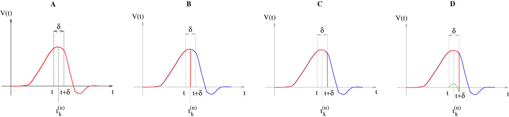
Figure 1. (A) “Real spike” shape; the sampling window is represented at a scale corresponding to a “small” sampling rate to enhance the related bias. (B) Spike shape for an integrate and fire model with instantaneous reset, the real shape is in blue. (C) Spike shape when reset occurs at time t + δ (Alternative I). (D) Spike shape with reset at time t + δ plus addition of the integrate current (green curve) (Alternative II).
In this paper we shall concentrate on Alternative II though mathematical results can be extended to Alternative I in a straightforward way. This corresponds to the initial choice of the Beslon–Mazet–Soula model (BMS) motivating the paper (Soula et al., 2006
) and the present work.
In this case, the reset corresponds to:

(recall that Vreset = 0).
IF regime can now be included in a unique equation, using the function Z defined in (11):

where we set δ = 1 from now on.
Examples
The Beslon–Mazet–Soula model
Consider the leaky IF model, where conductances are constant. Set  for excitatory (inhibitory) synapses. Then, replacing the α-profile by a Dirac distribution, (20) reduces to:
for excitatory (inhibitory) synapses. Then, replacing the α-profile by a Dirac distribution, (20) reduces to:
This model has been proposed by Soula et al. (2006)
. A mathematical analysis of its asymptotic dynamics has been done in Cessac (2008) and we extend these results to the more delicate case of conductance based IF models in the present paper. [Note that having constant conductances leads to a dynamics which is independent of the past firing times (raster plot). In fact, the dynamical system is essentially a cellular automaton but with a highly non trivial dynamics].
Alpha-profile conductances
Consider now a conductance based model of form (3), leading to:

where K is a constant:

while, using the form (6) for α gives:
One has therefore to handle an exponential of an exponential. This example illustrates one of the main problem in IF models. IF models have been introduced to simplify neurons description and to simplify numerical calculations [compared, e.g., with Hodgkin–Huxley’s model (Hodgkin and Huxley, 1952
)]. Indeed, their structure allows one to write an explicit expression for the next firing times of each neurons, knowing the membrane potential value. However, in case of α exponential profile, there is no simple form for the integral and, even in the case of one neuron, one has to use approximations with Γ functions (Rudolph and Destexhe, 2006
) which reduce consequently the interest of IF models and event based integration schemes.
The General Picture
In this section we develop in words some important mathematical aspects of the dynamical system (20), mathematically proved in the sequel.
Singularity set
The first important property is that the dynamics (20) (and the dynamics of continuous time IF models as well) is not smooth, but has singularities, due to the sharp threshold definition in neurons firing. The singularity set is:
This is the set of membrane potential vectors such that at least one of the neurons has a membrane potential exactly equal to the threshold
[9
. This set has a simple structure: it is a finite union of N − 1 dimensional hyperplanes. Although  is a “small” set both from the topological (non residual set) and metric (zero Lebesgue measure) point of view, it has an important effect on the dynamics.
is a “small” set both from the topological (non residual set) and metric (zero Lebesgue measure) point of view, it has an important effect on the dynamics.Local contraction
The other important aspect is that the dynamics is locally contracting, because  (see Eq. (18)). This has the following consequence. Let us consider the trajectory of a point V ∈ and perturbations with an amplitude <ε about V (this can be some fluctuation in the current, or some additional noise, but it can also be some error due to a numerical implementation). Equivalently, consider the evolution of the ε-ball
  (V, ε). If (V, ε) ∩ =
  then we shall see in the next section that the image of (V, ε) is a ball with a smaller diameter. This means, that, under the condition (V, ε) ∩ = , a perturbation is damped. Now, if the images of the ball under the dynamics never intersect , any ε-perturbation around V is exponentially damped and the perturbed trajectories about V become asymptotically indistinguishable from the trajectory of V. Actually, there is a more dramatic effect. If all neurons have fired after a finite time t then all perturbed trajectories collapse onto the trajectory of V after t + 1 iterations (see prop. 1 below).
(see Eq. (18)). This has the following consequence. Let us consider the trajectory of a point V ∈ and perturbations with an amplitude <ε about V (this can be some fluctuation in the current, or some additional noise, but it can also be some error due to a numerical implementation). Equivalently, consider the evolution of the ε-ball (V, ε). If (V, ε) ∩ = then we shall see in the next section that the image of (V, ε) is a ball with a smaller diameter. This means, that, under the condition (V, ε) ∩ = , a perturbation is damped. Now, if the images of the ball under the dynamics never intersect , any ε-perturbation around V is exponentially damped and the perturbed trajectories about V become asymptotically indistinguishable from the trajectory of V. Actually, there is a more dramatic effect. If all neurons have fired after a finite time t then all perturbed trajectories collapse onto the trajectory of V after t + 1 iterations (see prop. 1 below).Initial conditions sensitivity
On the opposite, assume that there is a time, t0, such that the image of the ball (V, ε) intersects . By definition, this means that there exists a subset of neurons {i1 ,…, ik} and V′ ∈ (V, ε), such that  , i ∈ {i1 ,…, ik}. For example, some neuron does not fire when not perturbed but the application of an ε-perturbation induces it to fire (possibly with a membrane potential strictly above the threshold). This requires obviously this neuron to be close enough to the threshold. Clearly, the evolution of the unperturbed and perturbed trajectory may then become drastically different (see Figure 2
). Indeed, even if only one neuron is lead to fire when perturbed, it may induce other neurons to fire at the next time step, etc …, inducing an avalanche phenomenon leading to unpredictability and initial condition sensitivity
[10
.
, i ∈ {i1 ,…, ik}. For example, some neuron does not fire when not perturbed but the application of an ε-perturbation induces it to fire (possibly with a membrane potential strictly above the threshold). This requires obviously this neuron to be close enough to the threshold. Clearly, the evolution of the unperturbed and perturbed trajectory may then become drastically different (see Figure 2
). Indeed, even if only one neuron is lead to fire when perturbed, it may induce other neurons to fire at the next time step, etc …, inducing an avalanche phenomenon leading to unpredictability and initial condition sensitivity
[10
.
(V, ε) intersects . By definition, this means that there exists a subset of neurons {i1 ,…, ik} and V′ ∈ (V, ε), such that , i ∈ {i1 ,…, ik}. For example, some neuron does not fire when not perturbed but the application of an ε-perturbation induces it to fire (possibly with a membrane potential strictly above the threshold). This requires obviously this neuron to be close enough to the threshold. Clearly, the evolution of the unperturbed and perturbed trajectory may then become drastically different (see Figure 2
). Indeed, even if only one neuron is lead to fire when perturbed, it may induce other neurons to fire at the next time step, etc …, inducing an avalanche phenomenon leading to unpredictability and initial condition sensitivity
[10
.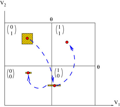
Figure 2. Schematic representation, for two neurons, of the natural partition and the mapping discussed in the text. In this case, a firing state is a vector with components  labeling the partition elements. A set of initial conditions, say a small (L∞) ball in , is contracted by leak (neuron 1 in the example) and reset (neuron 2 in the example), but its image can intersect the singularity set. This generates several branches of trajectories. Note that we have given some width to the projection of the image of the ball on direction 2 in order to see it on the picture. But since neuron 2 fires the width is in fact 0.
and the mapping discussed in the text. In this case, a firing state is a vector with components labeling the partition elements. A set of initial conditions, say a small (L∞) ball in , is contracted by leak (neuron 1 in the example) and reset (neuron 2 in the example), but its image can intersect the singularity set. This generates several branches of trajectories. Note that we have given some width to the projection of the image of the ball on direction 2 in order to see it on the picture. But since neuron 2 fires the width is in fact 0.It is tempting to call this behavior “chaos”, but there is an important difference with the usual notion of chaos in differentiable systems. In the present case, due to the sharp condition defining the threshold, initial condition only occurs at sporadic instants, whenever some neuron is close enough to the threshold. Indeed, in certain periods of time the membrane potential typically is quite far below threshold, so that the neuron can fire only if it receives strong excitatory input over a short period of time. It shows then a behavior that is robust against fluctuations. On the other hand, when membrane potential is close to the threshold a small perturbation may induce drastic change in the evolution.
Stability with respect to small perturbations
Therefore, depending on parameters such as the synaptic weights, the external current, it may happen that, in the stationary regime, the typical trajectories stay away from the singularity set, say within a distance larger than ε > 0, which can be arbitrary small, (but positive). Thus, a small perturbation (smaller than ε) does not produce any change in the evolution. At a computational level, this robustness leads to stable input-output transformations. In this case, as we shall see, the dynamics of (20) is asymptotically periodic (but there may exist a large number of possible orbits, with a large period). In this situation the system has a vanishing entropy
[11
. This statement is made rigorous in theorem 1 below.
On the other hand, if the distance between the set where the asymptotic dynamics lives
[12
and the singularity set is arbitrary small then the dynamics exhibit initial conditions sensitivity, and chaos. Thus, a natural question is: is chaos a generic situation? How does this depend on the parameters? A related question is: how does the numerical errors induced by a time discretization scheme evolve under dynamics (Hansel et al., 1998
)?
Edge of chaos
It has been shown, in Cessac (2008)
for the BMS model, that there is a sharp transition
[13
from fixed point to complex dynamics, when crossing a critical manifold usually called the “edge of chaos” in the literature. While this notion is usually not sharply defined in the Neural Network literature, we shall give a mathematical definition which is moreover tractable numerically. Strictly speaking chaos only occurs on this manifold, but from a practical point of view, the dynamics is indistinguishable
[14
from chaos, close to this manifold. When the distance to the edge of chaos further increases the dynamics is periodic with typical periods compatible with simulation times. This manifold can be characterized in the case where the synaptic weights are independent, identically distributed with a variance  .
.
.In BMS model (e.g., time discretized gIF model with constant conductances) it can be proved that the chaotic situation is non generic (Cessac, 2008
). We now develop the same lines of investigation and discuss how these result extend to the model (20). Especially, the “edge of chaos” is numerically computed and compared to the BMS situation.
Let us now switch to the related mathematical results. Proofs are given in the Appendix.
Piecewise Affine MAP
Let us first return to the notion of raster plot developed in Section 2. At time t, the firing state (t) ∈ Λ can take at most 2N values. Thus, the list of firing states (0) ,…, (t) ∈ Λt + 1 can take at most 2N(t + 1) values. (In fact, as discussed below, only a subset of these possibilities is selected by the dynamics). This list is the raster plot up to time t and we have denoted by  . Once the raster plot up to time t has been fixed the coefficients γk and the integrated currents Jk in (20) are determined. Fixing the raster plot up to time t amounts to construct branches for the discrete flow of the dynamics, corresponding to sub-domains of constructed iteratively, via the natural partition (9), in the following way.
(t) ∈ Λ can take at most 2N values. Thus, the list of firing states (0) ,…, (t) ∈ Λt + 1 can take at most 2N(t + 1) values. (In fact, as discussed below, only a subset of these possibilities is selected by the dynamics). This list is the raster plot up to time t and we have denoted by . Once the raster plot up to time t has been fixed the coefficients γk and the integrated currents Jk in (20) are determined. Fixing the raster plot up to time t amounts to construct branches for the discrete flow of the dynamics, corresponding to sub-domains of constructed iteratively, via the natural partition (9), in the following way.Fix t > 0 and . Note:
. Note:
This is the set (possibly empty) of initial membrane potentials vectors V ≡ V(0) whose firing pattern at time s is (s), s = 0,…, t. Consequently,  we have:
(s), s = 0,…, t. Consequently, we have:
as easily found by recursion on (20). We used the convention 
Then, define the map:
with Vk(t + 1) given by (25) and  . Note that
  is affine. Finally define:
. Note that is affine. Finally define:
such that the restriction of Ft + 1 to the domain  is precisely
  . This mapping is the flow of the model (20) where:
is precisely . This mapping is the flow of the model (20) where:V(t + 1) = Ft + 1 V, V ∈
A central property of this map is that it is piecewise affine and it has at most 2N(t + 1) branches  parameterized by the legal sequences
  which parameterize the possible histories of the conductance/currents up to time t.
parameterized by the legal sequences which parameterize the possible histories of the conductance/currents up to time t.Let us give a bit of explanation of this construction. Take  . This amounts to fixing the firing pattern at time 0 with the relation
  . Therefore,
  , where γk, Jk do not depend on V(0) but only on the spike state of neurons at time 0. Therefore, the mapping
  such that
  is affine (and continuous on the interior of
  ). Since (0) is an hypercube,
  is a convex connected domain. This domain typically intersects several domains of the natural partition . This corresponds to the following situation. Though the pattern of neuron firing at time 0 is fixed as soon as
  , the list of neurons firing at the next time depends on the value of the membrane potentials V(0), and not only on the spiking pattern at time 0. But, by definition, the domain:
. This amounts to fixing the firing pattern at time 0 with the relation . Therefore, , where γk, Jk do not depend on V(0) but only on the spike state of neurons at time 0. Therefore, the mapping such that is affine (and continuous on the interior of ). Since (0) is an hypercube, is a convex connected domain. This domain typically intersects several domains of the natural partition . This corresponds to the following situation. Though the pattern of neuron firing at time 0 is fixed as soon as , the list of neurons firing at the next time depends on the value of the membrane potentials V(0), and not only on the spiking pattern at time 0. But, by definition, the domain:
is such that  , the spiking pattern at time 0 is (0) and it is (1) at time 1. If the intersection is empty this simply means that one cannot find a membrane potential vector such that neurons fire according to the spiking pattern (0) at time t = 0 then fire according to the spiking pattern (1) at time t = 1. If the intersection is not empty we say that “the transition (0) → (1) is legal”
[15
.
, the spiking pattern at time 0 is (0) and it is (1) at time 1. If the intersection is empty this simply means that one cannot find a membrane potential vector such that neurons fire according to the spiking pattern (0) at time t = 0 then fire according to the spiking pattern (1) at time t = 1. If the intersection is not empty we say that “the transition (0) → (1) is legal”
[15
.Proceeding recursively as above one constructs a hierarchy of domains  and maps
  . Incidentally, an equivalent definition of is:
and maps . Incidentally, an equivalent definition of is:
As stated before, is the set of membrane potential vectors V such that the firing patterns up to time t are (0) ,…, (t). If this set is non empty we say that the sequence (0) ,…, (t) is legal. Though there are at most 2N(t + 1) possible raster plots at time t the number of legal raster plots is typically smaller. This number can increase either exponentially with t or slower. We shall denote by  the set of all legal (infinite) raster plots (legal infinite sequences of firing states). Note that is a topological space for the product topology generated by cylinder sets (Katok and Hasselblatt, 1998
). The set
the set of all legal (infinite) raster plots (legal infinite sequences of firing states). Note that is a topological space for the product topology generated by cylinder sets (Katok and Hasselblatt, 1998
). The set  of raster plots having the same first t + 1 firing patterns is a cylinder set.
is the set of membrane potential vectors V such that the firing patterns up to time t are (0) ,…, (t). If this set is non empty we say that the sequence (0) ,…, (t) is legal. Though there are at most 2N(t + 1) possible raster plots at time t the number of legal raster plots is typically smaller. This number can increase either exponentially with t or slower. We shall denote by the set of all legal (infinite) raster plots (legal infinite sequences of firing states). Note that is a topological space for the product topology generated by cylinder sets (Katok and Hasselblatt, 1998
). The set of raster plots having the same first t + 1 firing patterns is a cylinder set.Phase Space Contraction
Now, we have the following:
Proposition 1. For all  , the mapping
 is affine, with a Jacobian matrix and an affine constant depending on
  . Moreover, the Jacobian matrix is diagonal with eigenvalues
, the mapping is affine, with a Jacobian matrix and an affine constant depending on . Moreover, the Jacobian matrix is diagonal with eigenvalues
Consequently,  is a contraction.
is a contraction.Proof. The proof results directly from the definition (26) and (25) with  [see (18)].
[see (18)].Since the domains of the natural partition are convex and connected, and since F is affine on each domain (therefore continuous on its interior), there is a straightforward corollary:
of the natural partition are convex and connected, and since F is affine on each domain (therefore continuous on its interior), there is a straightforward corollary:Corrollary 1. The domains  are convex and connected.
are convex and connected.There is a more important, but still straightforward consequence:
Corrollary 2. Ft+1 is a non uniform contraction on where the contraction rate in direction k is  ,
,  .
.
where the contraction rate in direction k is , .Then, we have the following:
Proposition 2. Fix  .
.
.1. If ∃t < ∞, such that, ∀k = 1 ,…, N, ∃s ≡ s(k) ≤ t where k(s) = 1 then  is a point. That is, all orbits born from the domain
  converge to the same orbit in a finite time.
k(s) = 1 then is a point. That is, all orbits born from the domain converge to the same orbit in a finite time.2. If  such that ∀t > 0, k(t) = 0 then
  is contracting in direction k, with a Lyapunov exponent
  , such that:
such that ∀t > 0, k(t) = 0 then is contracting in direction k, with a Lyapunov exponent , such that:
Proof. Statement 1 holds since, under these hypotheses, all eigenvalues of  are 0. For 2, since
  is diagonal, the Lyapunov exponent in direction k is defined by
 whenever the limit exists (it exists almost surely for any F invariant measure from Birkhoff theorem).
are 0. For 2, since is diagonal, the Lyapunov exponent in direction k is defined by whenever the limit exists (it exists almost surely for any F invariant measure from Birkhoff theorem).Remark
An alternative definition of Lyapunov exponent has been introduced by Coombes (1999a
,b
), for IF neurons. His definition, based on ideas developed for impact oscillators (Muller, 1995
), takes care of the discontinuity in the trajectories arising when crossing . Unfortunately, his explicit computation at the network level (with continuous time dynamics), makes several implicit assumptions [see Eq. 6 in Coombes (1999a)
: (1) there is a finite number of spikes within a bounded time interval; (2) the number of spikes that have been fired up to time t, ∀t > 0, is the same for the mother trajectory and for a daughter trajectory, generated by a small perturbation of the mother trajectory at t = 0; (3) call  , in Coombes’ notations, the kth spike time for neuron i in the mother trajectory, and
  the kth spike time for neuron i in the daughter trajectory. Then
  , where
  is assumed to become arbitrary small, ∀k ≥ 0, when the initial perturbation amplitude tends to 0. While assumption (1) can be easily fulfilled (e.g., by adding a refractory period) assumptions (2) and (3) are more delicate.
. Unfortunately, his explicit computation at the network level (with continuous time dynamics), makes several implicit assumptions [see Eq. 6 in Coombes (1999a)
: (1) there is a finite number of spikes within a bounded time interval; (2) the number of spikes that have been fired up to time t, ∀t > 0, is the same for the mother trajectory and for a daughter trajectory, generated by a small perturbation of the mother trajectory at t = 0; (3) call , in Coombes’ notations, the kth spike time for neuron i in the mother trajectory, and the kth spike time for neuron i in the daughter trajectory. Then , where is assumed to become arbitrary small, ∀k ≥ 0, when the initial perturbation amplitude tends to 0. While assumption (1) can be easily fulfilled (e.g., by adding a refractory period) assumptions (2) and (3) are more delicate.Transposing this computation to the present analysis, this requires that both trajectories are never separated by the singularity set. A sufficient condition is that the mother trajectory stays sufficiently far from the singularity set. In this case the Lyapunov exponent defined by Coombes coincides with our definition and it is negative. On the other hand, in the “chaotic” situation (see Section 3), assumptions (2) and (3) can typically fail. For example, it is possible that neuron i stops firing after a certain time, in the daughter trajectory, while it was firing in the mother trajectory, and this can happen even if the perturbation is arbitrary small. This essentially means that the explicit formula for the Lyapunov exponent proposed in Coombes (1999a)
cannot be applied as well in the “chaotic” regime.
Asymptotic Dynamics
Attracting set  and -limit set
and -limit setThe main notion that we shall be interested in from now on concerns the invariant set where the asymptotic dynamics lives.
Definition 1 (From Guckenheimer and Holmes, 1983 and Katok and Hasselblatt, 1998
)
A point y ∈ is called an -limit point for a point x ∈ if there exists a sequence of times  , such that x(tk) → y as tk → + ∞. The -limit set of x, (x), is the set of all -limit points of x. The -limit set of , denoted by Ω, is the set
  .
.
is called an -limit point for a point x ∈ if there exists a sequence of times , such that x(tk) → y as tk → + ∞. The -limit set of x, (x), is the set of all -limit points of x. The -limit set of , denoted by Ω, is the set .Equivalently, since is closed and invariant, we have  .
.
is closed and invariant, we have .Basically, Ω is the union of attractors. But for technical reasons, related to the case considered in Section 3, it is more convenient to use the notion of -limit set.
-limit set.A theorem about the structure of Ω
Theorem 1. Assume that ∃ε > 0 and ∃T < ∞ such that, ∀V∈ , ∀i∈{1 ,…, N},
, ∀i∈{1 ,…, N},1. Either ∃t ≤ T such that Vi(t) ≥ θ;
2. Or ∃t0 ≡ t0(V, ε)such that ∀t ≥ t0, Vi(t) < θ − ε
Then, Ω is composed by finitely many periodic orbits with a period ≤T.
The proof is given in the Appendix 2.
Note that conditions (1) and (2) are not disjoint. The meaning of these conditions is the following. (1) corresponds to imposing that a neuron has fired after a finite time T (uniformly bounded, i.e., independent of V and i). (2) amounts to requiring that after a certain time t0, the membrane potential stays below the threshold value and it cannot accumulate on θ. We essentially want to avoid a situation when a neuron can fire for the first time after an unbounded time (see Section 3 for a discussion of this case). Thus assumptions (1) and (2) look quite reasonable. Under these assumptions the asymptotic dynamics is periodic and one can predict the evolution after observing the system on a finite time horizon T, whatever the initial condition. Note however that T can be quite a bit large.
There is a remarkable corollary result, somehow hidden in the proof given in the Appendix. The neurons that do not fire after a finite time are still driven by the dynamics of firing neurons. It results that, in the asymptotic regime, non firing neurons have a membrane potential which oscillates below the threshold. This exactly corresponds to what people call “sub-threshold oscillations”. In particular, there are times where those membrane potentials are very close to the threshold, and a small perturbation can completely changes further evolution. This issue is developed in the next section. Possible biological interpretations are presented in the discussion section.
Ghost orbits
The advantage of the previous theorem is that we define conditions where one can relatively easily controls dynamics. However, what happens if we consider the complementary situation corresponding to the following definition?
Definition 2 An orbit  is a ghost orbit if ∃i such that:
is a ghost orbit if ∃i such that:(i) ∀t > 0, Vi(t) < θ
and
Namely there exists at least one initial condition V and one neuron i such that one cannot uniformly bound the first time of firing, and Vi(t) approaches arbitrary close the threshold. In other words sub-threshold oscillations drive the neuron “dangerously close” to the threshold, though we are not able to predict when the neuron will fire. This may look a “strange” case from a practical point of view, but it has deep implications. This indeed means that we can observe the dynamics on arbitrary long times without being able to predict what will happen later on, because when this neuron eventually fire, it may drastically change the evolution. This case is exactly related to the chaotic or unpredictable regime of IF models.
One may wonder whether the existence of ghost orbits is “generic”. To reply to this question one has first to give a definition of genericity. In the present context, it is natural to consider the dynamical system describing the time evolution of our neural network as a point in a space  of parameters. These parameters can be, e.g., the synaptic weights, or parameters fixing the time scales, the reversal potentials, the external currents, etc… Varying these parameters (i.e., moving the point representing our dynamical system in ) can have two possible effects. Either there is no qualitative change in the dynamics and observable quantities such as, e.g., firing rates, average inter-spikes interval, etc, are varying continuously. Or, a sharp change (bifurcation) occurs. This corresponds to the crossing of a critical or bifurcation manifold in . Now, a behavior is generic if it is “typical”. On mathematical grounds this can have two meanings. Either this behavior is obtained, with a positive probability, when drawing the parameters (the corresponding point in ) at random with some natural probability (e.g., Gaussian). In this case one speaks of “metric genericity”. Or, this behavior holds in a dense subset of . One speaks then of “topological genericity”. The two notions usually do not coincide.
of parameters. These parameters can be, e.g., the synaptic weights, or parameters fixing the time scales, the reversal potentials, the external currents, etc… Varying these parameters (i.e., moving the point representing our dynamical system in ) can have two possible effects. Either there is no qualitative change in the dynamics and observable quantities such as, e.g., firing rates, average inter-spikes interval, etc, are varying continuously. Or, a sharp change (bifurcation) occurs. This corresponds to the crossing of a critical or bifurcation manifold in . Now, a behavior is generic if it is “typical”. On mathematical grounds this can have two meanings. Either this behavior is obtained, with a positive probability, when drawing the parameters (the corresponding point in ) at random with some natural probability (e.g., Gaussian). In this case one speaks of “metric genericity”. Or, this behavior holds in a dense subset of . One speaks then of “topological genericity”. The two notions usually do not coincide.In the BMS model, ghost orbits are non generic in both senses (Cessac, 2008
). The proof does not extend to more general models such as (20) because it heavily uses the fact that the synaptic current takes only finitely many values in the BMS model. As soon as we introduce a dependence in  this is not the case anymore. We do not know yet how to extend this proof.
this is not the case anymore. We do not know yet how to extend this proof.Edge of Chaos
On practical grounds ghost orbits involve a notion of limit t → +∞ which has no empirical meaning. Therefore the right question is: are there situations where a neuron can fire for the first time after a time which is well beyond the observation time? One way to analyze this effect is to consider how close the neurons are to the threshold in their evolution. On mathematical grounds this is given by the distance from the singularity set to the ω-limit set:

The advantage of this definition, is that it can easily be adapted to the plausible case where observation time is bounded (see Section 3).
Now, the following theorem holds.
Theorem 2.
- If d(Ω, ) > 0 then Ω is composed by finitely many periodic orbits with a finite period.
- There is a one-to-one correspondence between a trajectory on Ω and its raster plot.
The proof is exactly the same as in (Cessac, 2008
) so we do not reproduce it here. It uses the fact that if d(Ω, ) > 0 then there is a finite time T, depending on d(Ω, ) and diverging as d(Ω, ) → 0, such that FT has a Markov partition (constituted by local stable manifolds since dynamics is contracting) where the elements of the partition are the domains  . Note, however, that d(Ω, ) > 0 is a sufficient but not a necessary condition to have a periodic dynamics. In particular, according to theorem 1 one can have d(Ω, ) = 0 and still have a periodic dynamics, if at some finite time t, for some neuron i, Vi(t) = θ. This strict equality is however not structurally stable, since a slight change, e.g., in the parameters will remove it. The main role of the condition d(Ω, ) > 0 is therefore to avoid situations where the membrane potential of some neuron accumulates on θ from below (ghost orbits). See the discussion section for a possible biological interpretation on this.
) > 0 then there is a finite time T, depending on d(Ω, ) and diverging as d(Ω, ) → 0, such that FT has a Markov partition (constituted by local stable manifolds since dynamics is contracting) where the elements of the partition are the domains . Note, however, that d(Ω, ) > 0 is a sufficient but not a necessary condition to have a periodic dynamics. In particular, according to theorem 1 one can have d(Ω, ) = 0 and still have a periodic dynamics, if at some finite time t, for some neuron i, Vi(t) = θ. This strict equality is however not structurally stable, since a slight change, e.g., in the parameters will remove it. The main role of the condition d(Ω, ) > 0 is therefore to avoid situations where the membrane potential of some neuron accumulates on θ from below (ghost orbits). See the discussion section for a possible biological interpretation on this.But d(Ω, ) plays another important role concerning the effect of perturbations on the dynamics. Indeed, if d(Ω, ) > 0 then the contraction property (corollary 2) implies that any perturbation smaller than d(Ω, ) will be damped by dynamics. In particular, making a small error on the spike time, or any other type of error leading to an indeterminacy of V smaller than d(Ω, ) will be harmless.
) plays another important role concerning the effect of perturbations on the dynamics. Indeed, if d(Ω, ) > 0 then the contraction property (corollary 2) implies that any perturbation smaller than d(Ω, ) will be damped by dynamics. In particular, making a small error on the spike time, or any other type of error leading to an indeterminacy of V smaller than d(Ω, ) will be harmless.Let us now discuss the second item of theorem 2. It expresses that the raster plot is a symbolic coding for the membrane potential trajectory. In other words there is no loss of information on the dynamics when switching from the membrane potential description to the raster plot description. This is not true anymore if d(Ω, ) = 0.
) = 0.The first item tells us that dynamics is periodic, but period can be arbitrary long. Indeed, following (Cessac, 2008
) an estimate for an upper bound on the orbits period is given by:

where <γ> denotes the value of γ averaged over time and initial conditions
[16
(see Appendix for details). Though this is only an upper bound this suggests that periods diverge when d(Ω, ) → 0. In BMS model, this is consistent with the fact that when d(Ω, ) is close to 0 dynamics “looks chaotic”. Therefore, d(Ω, ) is what a physicist could call an “order parameter”, quantifying somehow the dynamics complexity. The distance d(Ω, ) can be numerically estimated as done in (33) and (34), Section 3.
) → 0. In BMS model, this is consistent with the fact that when d(Ω, ) is close to 0 dynamics “looks chaotic”. Therefore, d(Ω, ) is what a physicist could call an “order parameter”, quantifying somehow the dynamics complexity. The distance d(Ω, ) can be numerically estimated as done in (33) and (34), Section 3.Before, we need the following list of (operational) definitions.
Definition 3 (Edge of chaos)
The edge of chaos is the set of points  in the parameter space where d(Ω, ) = 0.
in the parameter space where d(Ω, ) = 0.The topological structure of can be quite complicated as we checked in the simplest examples (e.g., the BMS model with Laplacian coupling) and suggested by the papers (Bressloff and Coombes, 2000a
,b
) (see Discussion). There are good reasons to believe that this set coincides with the set of points where the entropy is positive [see Kruglikov and Rypdal (2006a
,b
) and discussion below]. The set of points where the entropy is positive can have a fractal structure even in the simplest examples of one dimensional maps (Mackay and Tresser, 1986
; Gambaudo and Tresser, 1988
). Therefore, there is no hope to characterize rigorously in a next future. Instead, we use below a numerical characterization.
can be quite complicated as we checked in the simplest examples (e.g., the BMS model with Laplacian coupling) and suggested by the papers (Bressloff and Coombes, 2000a
,b
) (see Discussion). There are good reasons to believe that this set coincides with the set of points where the entropy is positive [see Kruglikov and Rypdal (2006a
,b
) and discussion below]. The set of points where the entropy is positive can have a fractal structure even in the simplest examples of one dimensional maps (Mackay and Tresser, 1986
; Gambaudo and Tresser, 1988
). Therefore, there is no hope to characterize rigorously in a next future. Instead, we use below a numerical characterization.The edge of chaos is a non generic set in the BMS model, and the same could hold as well in model (20). Nevertheless, it has a strong influence on the dynamics, since crossing it leads to drastic dynamical changes. Moreover, close to dynamics can be operationally indistinguishable from chaos. More precisely, let us now propose another definition.
dynamics can be operationally indistinguishable from chaos. More precisely, let us now propose another definition.Definition 4 (Effective entropy)
Fix T0 called “the observational time”. This is the largest accessible duration of an experiment. Call n(t) the number of (legal) truncated raster plots up to time t. Then, the effective entropy is;

Note that in the cases where raster plots provide a symbolic coding for the dynamics then  , the topological entropy.
, the topological entropy.On practical grounds, this definition corresponds to the following notion. The larger the effective entropy, the more the system is able to produce distinct neural codes. This provides one way to measure the “complexity” of the dynamics. On more “neuronal” grounds this quantity measures the variability in the dynamical response of the neuronal network to a given stimulus (external current) or its ability to produce distinct “functions” (a function being the response to a stimulus in terms of a spikes train). Thinking of learning mechanisms (e.g., Hebbian) and synaptic plasticity (LTD, LTP, STDP) one may expect to having the largest learning capacities when this entropy is large. This aspect will be developed in a separated paper (for the effect of Hebbian learning and entropy reduction in firing rate neural networks see Siri et al., 2008
).
Finally, a positive effective entropy means that the system essentially behaves like a chaotic system during the time of the experiment. Indeed, the entropy is closely related to the distance d(Ω, ), since, from (30), a rough estimate/bound of h(eff) is easily obtained from (30), (31):
), since, from (30), a rough estimate/bound of h(eff) is easily obtained from (30), (31):
The notion of effective entropy provides some notion of “width” to the edge of chaos . For a fixed T0 the system behaves chaotically in a thick region  in such that h(eff) > 0. And from (32) one expects that this entropy gets larger when d(Ω, ) gets smaller.
. For a fixed T0 the system behaves chaotically in a thick region in such that h(eff) > 0. And from (32) one expects that this entropy gets larger when d(Ω, ) gets smaller.Effects of Time Discretization
Under the light of the previous results, let us reconsider the approximation where spikes are taken into account at multiple of the characteristic time scale δ, for the conductances update. Doing this, we make some error in the computation of the membrane potential, compared to the value obtained when using the “exact” spike time value. Now, the question is whether this error will be amplified by the dynamics, or damped. As we saw, dynamics (20) is contracting but the effect of a small error can have dramatic consequences when approaching the singularity set. The distance d(Ω, ) provides a criterion to define a “safe” region where a small error of amplitude ε > 0 in the membrane potential value is harmless, basically, if ε < d(Ω, ). On the other hand, if we are in a region of the parameters space where d(Ω, ) = 0 then a slight perturbation has an incidence on the further evolution. Since δ can be arbitrary small in our theorems we have a good control on the dynamics of the continuous time IF models except at the edge of chaos where d(Ω, ) = 0. This enhances the question of mathematically characterizing this region in the parameter space . Note indeed that numerical investigations are of little help here since we are looking for a parameter region where the distance d(Ω, ) defined as an asymptotic limit, has to be exactly 0. The problem is that even sophisticated schemes (e.g., event based) are also submitted to round off errors. Therefore, as a conclusion, it might well be that all numerical schemes designed to approximate continuous time IF models display trajectory sensitivity to spike time errors, when approaching d(Ω, ) = 0.
) provides a criterion to define a “safe” region where a small error of amplitude ε > 0 in the membrane potential value is harmless, basically, if ε < d(Ω, ). On the other hand, if we are in a region of the parameters space where d(Ω, ) = 0 then a slight perturbation has an incidence on the further evolution. Since δ can be arbitrary small in our theorems we have a good control on the dynamics of the continuous time IF models except at the edge of chaos where d(Ω, ) = 0. This enhances the question of mathematically characterizing this region in the parameter space . Note indeed that numerical investigations are of little help here since we are looking for a parameter region where the distance d(Ω, ) defined as an asymptotic limit, has to be exactly 0. The problem is that even sophisticated schemes (e.g., event based) are also submitted to round off errors. Therefore, as a conclusion, it might well be that all numerical schemes designed to approximate continuous time IF models display trajectory sensitivity to spike time errors, when approaching d(Ω, ) = 0.A “Coarse-Grained” Characterization
As mentioned in the previous section an exact analytic computation of the edge of chaos in the general case seems to be out of reach. However, a “coarse grained” characterization can be performed at the numerical level and possibly some analytic approximation could be obtained. For this, we choose the synaptic weights (resp. the synaptic conductances) (and/or the external currents) randomly, with some probability  W (
W ( ), where
  is the matrix of synaptic weights (
 ) and i(ext) the vector of external currents (recall that external currents are time constant in this paper). A natural starting point is the use of Gaussian independent, identically distributed variables, where one varies the parameters, mean and variance, defining the probability definition [we call them statistical parameters, see Cessac and Samuelides (2007) and Samuelides and Cessac (2007)
for further developments on this approach]. Doing these, one performs a kind of fuzzy sampling of the parameters space, and one somehow expects the behavior observed for a given value of the statistical parameters to be characteristic of the region of , i(ext) that the probabilities
) and i(ext) the vector of external currents (recall that external currents are time constant in this paper). A natural starting point is the use of Gaussian independent, identically distributed variables, where one varies the parameters, mean and variance, defining the probability definition [we call them statistical parameters, see Cessac and Samuelides (2007) and Samuelides and Cessac (2007)
for further developments on this approach]. Doing these, one performs a kind of fuzzy sampling of the parameters space, and one somehow expects the behavior observed for a given value of the statistical parameters to be characteristic of the region of , i(ext) that the probabilities  weight [more precisely, one expects to observe a “prevalent” behavior in the sense of Hunt et al. (1992)
.
weight [more precisely, one expects to observe a “prevalent” behavior in the sense of Hunt et al. (1992)
.
W (), where is the matrix of synaptic weights () and i(ext) the vector of external currents (recall that external currents are time constant in this paper). A natural starting point is the use of Gaussian independent, identically distributed variables, where one varies the parameters, mean and variance, defining the probability definition [we call them statistical parameters, see Cessac and Samuelides (2007) and Samuelides and Cessac (2007)
for further developments on this approach]. Doing these, one performs a kind of fuzzy sampling of the parameters space, and one somehow expects the behavior observed for a given value of the statistical parameters to be characteristic of the region of , i(ext) that the probabilities weight [more precisely, one expects to observe a “prevalent” behavior in the sense of Hunt et al. (1992)
.The idea is then to estimate numerically d(Ω, ) in order to characterize how it varies when changing the statistical parameters. As an example, in the present paper, we select conductances (resp. synaptic weights) randomly with a Gaussian probability with a fixed mean and a variance  , and we study the behavior of d(Ω, ) when σ is varying. Note that the neural network is almost surely fully connected. We compute numerically an approximation of the distance d(Ω, ), where we fix a transient time Tr and an observation time To and average over several initial conditions V(n), n = 1 ,…, NCI for a given sample of synaptic weights. Then we perform an average over several synaptic weights samples m, m = 1 ,…, NW. In a more compact form, we compute:
) in order to characterize how it varies when changing the statistical parameters. As an example, in the present paper, we select conductances (resp. synaptic weights) randomly with a Gaussian probability with a fixed mean and a variance , and we study the behavior of d(Ω, ) when σ is varying. Note that the neural network is almost surely fully connected. We compute numerically an approximation of the distance d(Ω, ), where we fix a transient time Tr and an observation time To and average over several initial conditions V(n), n = 1 ,…, NCI for a given sample of synaptic weights. Then we perform an average over several synaptic weights samples m, m = 1 ,…, NW. In a more compact form, we compute:
where

In this way, we obtain a rough and coarse grained location of the edge of chaos where the distance d(Ω, ) vanishes.
) vanishes.We have performed the following experiments with two control parameters.
- Variance of random synaptic weights. We randomly select the synaptic strength which modulates the synaptic conductance using a Gaussian distribution so that 80% of the synapses are excitatory and 20% inhibitory. The average standard-variation σ is varied. The value σ = 0.5 corresponds, in our units, to what is chosen in the literature when considering the biological dispersion in the cortex (e.g., Rudolph and Destexhe, 2006 ). Note however that, at the present stage of investigation, Dale’s principle is not taken into account.
- Membrane leak time-constant. As an additional control parameter we vary the membrane leak around the usual τL = 1 ,…, 20 ms values. This choice is two-fold. The value τL = 20 ms corresponds to in vitro measurement, while τL → 1 ms allows to represent in vivo conditions in the cortex. On the other hand, it acts directly on the average contraction rate <γ> which is a natural control parameter.
Each simulation randomly selects the initial potential values in a −70 ,…, 30 mV range. For each condition the simulation is run for NCI = 100 initial conditions and N = 10 random selection of the synaptic weights. With a sampling period of 0.1 ms, the network is run during Tr = 1000 steps in order to “skip” the transients
[17
and then observed during To = 1000 steps. In order to explore the role of history dependent conductances on the dynamics we considered different models from the biologically plausible IF model to BMS model. More precisely we explore four modeling variants:
= 10 random selection of the synaptic weights. With a sampling period of 0.1 ms, the network is run during Tr = 1000 steps in order to “skip” the transients
[17
and then observed during To = 1000 steps. In order to explore the role of history dependent conductances on the dynamics we considered different models from the biologically plausible IF model to BMS model. More precisely we explore four modeling variants:
- Model I, defined in (20).
- Model II (20) with a fixed γ. The evolution equation of membrane potentials is thus given by:
where the average
 is the value observed during the numerical simulation of model I. Note that depends on the parameters σ, τL. The goal of this simulation is to check the role of the fluctuations of
  , controlling the instantaneous contraction rate, compared to a mean-field model where
  is replaced by its average. This corresponds to what is called “current based” synapses instead of “conductance based” synapses in the literature (see e.g., Brette et al., 2007
).
is replaced by its average. This corresponds to what is called “current based” synapses instead of “conductance based” synapses in the literature (see e.g., Brette et al., 2007
). - Model III (20) approximation with a fixed γ and simplified synapses. The evolution equation of membrane potentials is given by:
In addition to the previous simplification, we consider so-called “current jump” synapses where the synaptic input simply corresponds to an impulse, added to the membrane potential equation. Here the magnitude of the impulse and its delay δ− = 2 ms and δ+ = 10 ms in order to keep both characteristics as closed as possible to the previous condition.
- Model IV (20) with a fixed γ and instantaneous simplified synapses. The evolution equation of membrane potentials is given by:
where in addition to the previous simplification, the delay has been suppressed and where
 . This last condition strictly correspond to the original BMS model (Soula et al., 2006
).
. This last condition strictly correspond to the original BMS model (Soula et al., 2006
).
The results are given below. We have first represented the average value  for the model I in the range σ ∈[0.01, 1], τL ∈[10, 40]ms (see Figure 3
). The quantity related to the contraction rate, is remarkably constant (with small variations within the range [0.965, 0.995]).
for the model I in the range σ ∈[0.01, 1], τL ∈[10, 40]ms (see Figure 3
). The quantity related to the contraction rate, is remarkably constant (with small variations within the range [0.965, 0.995]).
for the model I in the range σ ∈[0.01, 1], τL ∈[10, 40]ms (see Figure 3
). The quantity related to the contraction rate, is remarkably constant (with small variations within the range [0.965, 0.995]).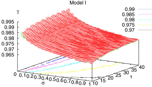
Figure 3. Average value of γ for model I σ ∈[0. 01, 1], τL∈[10, 40]ms. The profile is very similar for other models.
Then, we have considered the average value of the current  , averaged over time, initial conditions and neurons and denoted by I to alleviate the notations (Figure 4
), the logarithm of the distance d(Ω, ) (Figures 5 and 7
), and the average Inter Spike Interval (ISI, Figure 6
), for the four models. The main observations are the following. Average current and ISIs have essentially the same form for all models. This means that these quantities are not really relevant if one wants to discriminate the various models in their dynamical complexity.
, averaged over time, initial conditions and neurons and denoted by I to alleviate the notations (Figure 4
), the logarithm of the distance d(Ω, ) (Figures 5 and 7
), and the average Inter Spike Interval (ISI, Figure 6
), for the four models. The main observations are the following. Average current and ISIs have essentially the same form for all models. This means that these quantities are not really relevant if one wants to discriminate the various models in their dynamical complexity.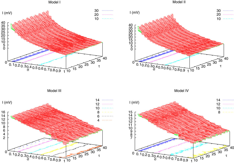
Figure 4. Average current I for the models I (top left)-II (top right)- III (bottom left)- IV (bottom right) with σ ∈[0. 01, 1], τL∈[10, 40]ms.
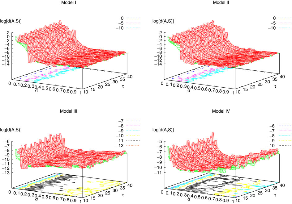
Figure 5. Average value of log[d(Ω, )] for the models I (top left)-II (top right)- III (bottom left)- IV (bottom right) with σ ∈[0.01, 1], τL∈[10, 40]ms.
)] for the models I (top left)-II (top right)- III (bottom left)- IV (bottom right) with σ ∈[0.01, 1], τL∈[10, 40]ms.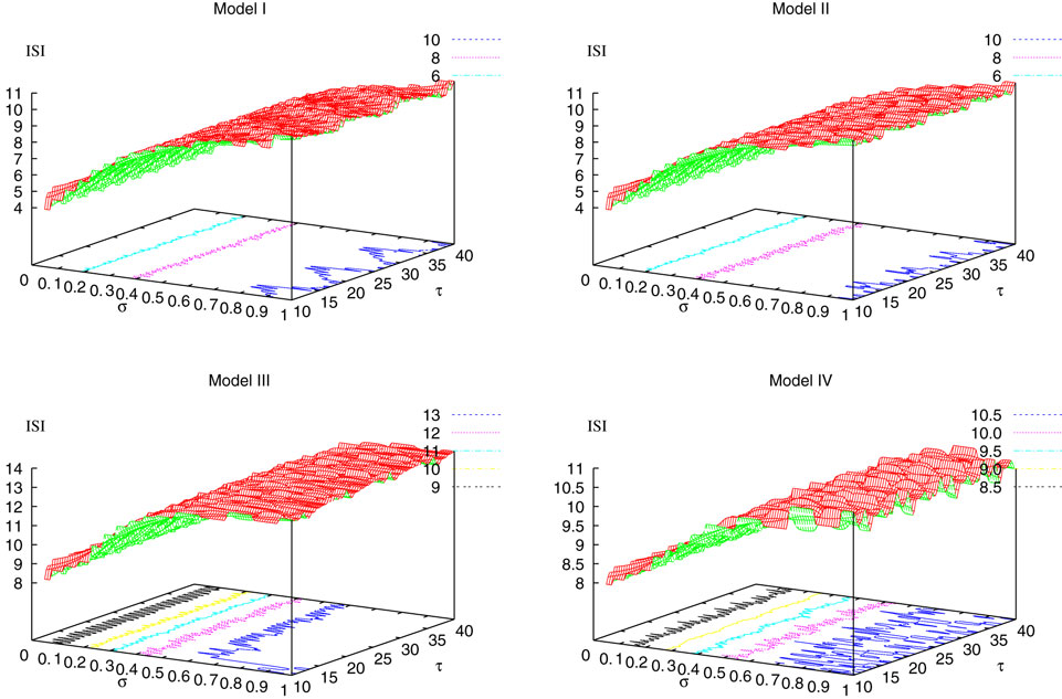
Figure 6. Average value of the ISI for the models I (top left)-II (top right)- III (bottom left)- IV (bottom right), with σ ∈[0.01, 1], τL∈[10, 40]ms.

Figure 7. Average value of log[d(Ω, )] for the model I (left) σ ∈[1, 10], τL∈[10, 40]ms. We present here a projection in the plane σ, log[d(Ω, )], and the vertical bars correspond to the variations with τL. It allows us to verify the stability of the previous result for higher variability of the synaptic weights. (middle) τL∈[1, 1 ,…, 2]ms below the usual 20 ms value, σ∈[1, 10]. Such range corresponds to cortical neurons in high-conductance state. It allows to check the behavior of d(Ω, ) in this case. (right) Sampling period of 1 ms, in order to verify the robustness of the numerical results with respect to the sampling rate.
)] for the model I (left) σ ∈[1, 10], τL∈[10, 40]ms. We present here a projection in the plane σ, log[d(Ω, )], and the vertical bars correspond to the variations with τL. It allows us to verify the stability of the previous result for higher variability of the synaptic weights. (middle) τL∈[1, 1 ,…, 2]ms below the usual 20 ms value, σ∈[1, 10]. Such range corresponds to cortical neurons in high-conductance state. It allows to check the behavior of d(Ω, ) in this case. (right) Sampling period of 1 ms, in order to verify the robustness of the numerical results with respect to the sampling rate.The observation of the distance d(Ω, ) is quite more interesting (Figure 7
). First, in the four models, the distance becomes very small when crossing some “critical region” in the plane τL, γ. This region has a regular structure for the BMS model, but its structure seems more complex for (20). Note however that the numerical investigations used here do not allow us to really conclude on this point. The most remarkable fact is that, in models III and IV, the distance increases when σ increases beyond this region, while it does not in models I and II. This corresponds to the following observation. When the d(Ω, ) is small, one observes a complex dynamics with no apparent period. One naturally concludes to a chaotic regime. As we saw, strictly speaking it is in fact periodic but since periods are well beyond observable times, the situation is virtually chaotic
[18
. When the distance increases, the orbits period decreases. Therefore, there is a range of σ values where period become smaller than observational time and one concludes that dynamics is periodic.
) is quite more interesting (Figure 7
). First, in the four models, the distance becomes very small when crossing some “critical region” in the plane τL, γ. This region has a regular structure for the BMS model, but its structure seems more complex for (20). Note however that the numerical investigations used here do not allow us to really conclude on this point. The most remarkable fact is that, in models III and IV, the distance increases when σ increases beyond this region, while it does not in models I and II. This corresponds to the following observation. When the d(Ω, ) is small, one observes a complex dynamics with no apparent period. One naturally concludes to a chaotic regime. As we saw, strictly speaking it is in fact periodic but since periods are well beyond observable times, the situation is virtually chaotic
[18
. When the distance increases, the orbits period decreases. Therefore, there is a range of σ values where period become smaller than observational time and one concludes that dynamics is periodic.The situation is different for models I and II since the distance does not apparently increases with σ. This suggests that introducing conductance based synapses and currents enhances considerably the width of the edge of chaos. On practical grounds, this means that models I and II have the capacity to display a very large number of distinct codes for wide choices of parameters. This is somewhat expected since the opposite conclusion would mean that introducing spike dependent conductances and current does not increases the complexity and information capacity of the system. But it is one thing to guess some behavior and another thing to measure it. Our investigations on the distance d(Ω, ), a concept based on the previous mathematical analysis, makes a step forward in this direction.
), a concept based on the previous mathematical analysis, makes a step forward in this direction.One step further, we have represented examples of raster plots in Figures 8 and 9
for models I and IV. The Figure 8
essentially illustrates the discussion above on the relation between the distance d(Ω, ) and the dynamics; for σ = 0.05, where d(Ω, ) is “large”, and dynamics is periodic; and for σ = 0.4, where d(Ω, ) is small, and dynamics looks more chaotic, for the two models. The difference between the two models becomes more accurate as σ increases. Figure 9
represents raster plots for models I and IV, with σ = 10, where we study the effect of a small amount of noise, of amplitude 10−4 × θ in the external current. This has no effect on model IV while it changes slightly the raster plot for model I, as expected. There is another remarkable difference. The code is sparser for model I than for model IV. This suggests that model I is in some sense optimal with respect to coding since it is able to detect very small changes in an input but the changes is not drastic and the neural code remains very sparse.
) and the dynamics; for σ = 0.05, where d(Ω, ) is “large”, and dynamics is periodic; and for σ = 0.4, where d(Ω, ) is small, and dynamics looks more chaotic, for the two models. The difference between the two models becomes more accurate as σ increases. Figure 9
represents raster plots for models I and IV, with σ = 10, where we study the effect of a small amount of noise, of amplitude 10−4 × θ in the external current. This has no effect on model IV while it changes slightly the raster plot for model I, as expected. There is another remarkable difference. The code is sparser for model I than for model IV. This suggests that model I is in some sense optimal with respect to coding since it is able to detect very small changes in an input but the changes is not drastic and the neural code remains very sparse.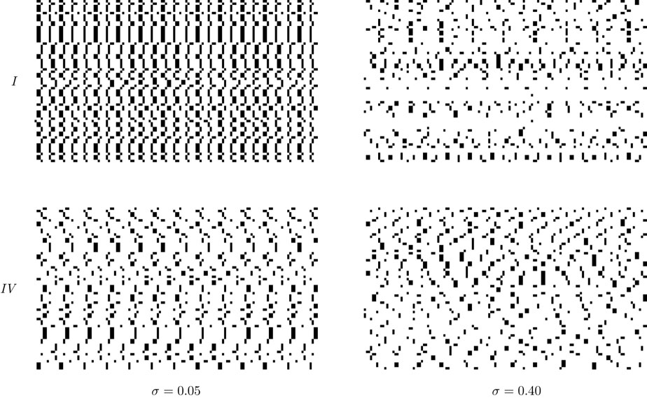
Figure 8. Examples of raster plots for the conductance based model (Model I, top row) and the leaky integrate and fire model (Model IV, bottom row). A time window of 100 samples is shown in each case. The control parameter is τL = 20 ms. As visible in Figure 5
, σ = 0.05 corresponds to a small order dynamics where the periodic behavior is clearly visible, and σ = 0.40 to the “edge of chaos”. One blob width is 1 msec.
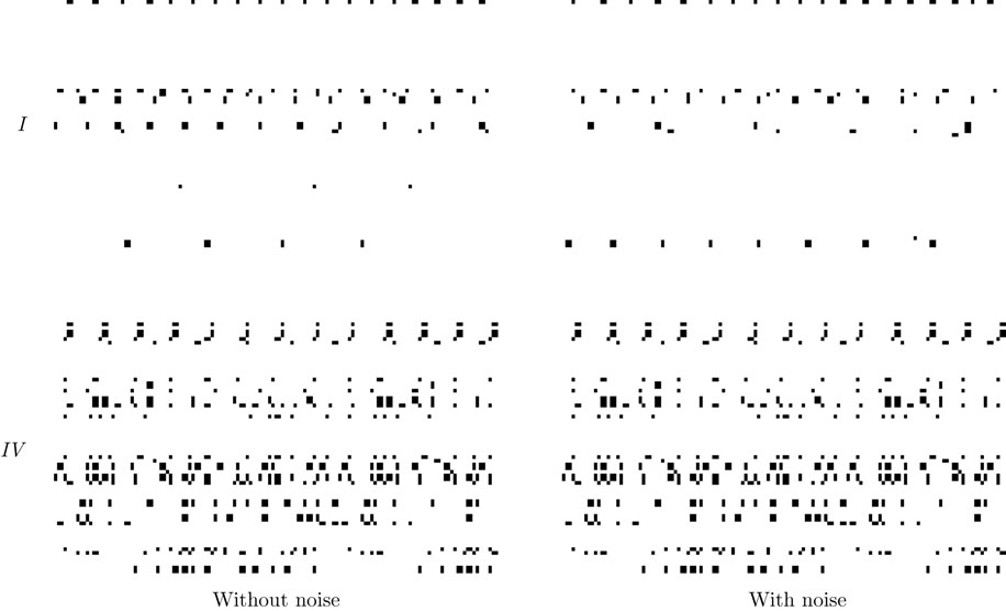
Figure 9. Raster plots for models I (upper row) and IV (lower row), with σ = 10.00 and the same condition as in Figure 8
. First column: model I and model without noise. Second column: same realization of synaptic weights and same initial conditions but with a small amount of noise in the external current. The noise is added to the membrane potential and its magnitude is very small (10−4 × θ). One blob width is 1 msec.
We have thus an operational definition for the “edge of chaos” where an “order parameter”, the distance of orbits to the singularity has been defined. This parameter has a deep meaning. It controls how much the system is sensitive to perturbations. Such perturbations can be noise, but they can also be a small variation in the external current, corresponding, e.g., to an input. If the amplitude of this perturbation is smaller than d(Ω, ) then it has no effect on the long term dynamics, and the neural code (raster plot) is unchanged. On the other hand, when the distance is small, even a tiny perturbation has a dramatic effect on the raster plot: the system produces a different code. As a corollary, the effective entropy is maximal when the distance is minimal. On practical ground, having a positive distance with a large effective entropy corresponds to situations where the system is able to produce a large number of distinct codes within the observational time, while this code is nevertheless robust to small perturbations of the input. Thus, we have a good compromise between the variability of the responses to distinct inputs and robustness of the code when an input is subject to small variations.
) then it has no effect on the long term dynamics, and the neural code (raster plot) is unchanged. On the other hand, when the distance is small, even a tiny perturbation has a dramatic effect on the raster plot: the system produces a different code. As a corollary, the effective entropy is maximal when the distance is minimal. On practical ground, having a positive distance with a large effective entropy corresponds to situations where the system is able to produce a large number of distinct codes within the observational time, while this code is nevertheless robust to small perturbations of the input. Thus, we have a good compromise between the variability of the responses to distinct inputs and robustness of the code when an input is subject to small variations.Several questions are now open. A first one concerns the way how we measured this distance. We used a random sampling with independent synaptic weights. But these weights are, in reality, highly correlated, via synaptic plasticity mechanism. What is the effect of, e.g., STPD or Hebbian learning on the effective entropy is a perspective for a future work. Recent results in Soula (2005) and Siri et al. (2007
, 2008)
suggest that synaptic plasticity reduces the entropy by diminishing the variability of raster plots and increasing the robustness of the response to an input. Some general (variational) mechanism could be at work here. This aspect is under investigation.
Another important issue is the effect of noise. It is usual in neural network modeling to add Brownian noise to the deterministic dynamics. This noise accounts for different effects such as the diffusion of neurotransmitters involved in the synaptic transmission, the degrees of freedom neglected by the model, external perturbations, etc… Though it is not evident that the “real noise” is Brownian, using this kind of perturbations has the advantage of providing a tractable model where standard theorems in the theory of stochastic processes (Touboul and Faugeras, 2007
) or methods in non equilibrium statistical physics [e.g., Fokker–Planck equations (Brunel and Hakim, 1999
)] can be applied.
Though we do not treat explicitly this case in the present work, the formalism has been designed to handle noise effects as well. As a matter of fact, the effect of Brownian noise on the dynamics of our model can be analyzed with standard techniques in probability theory and stochastic perturbations of dynamical systems (Freidlin and Wentzell, 1998
). In particular, the probability distribution of the membrane potential trajectory can be obtained by using a discrete time version of Girsanov theorem (Samuelides and Cessac, 2007
). Noise have several effects. Firstly, the stochastic trajectories stay around the unperturbed orbits until they jump to another attraction basin, the characteristic time depending on the noise intensity (“Arrhenius law”). This has the effect of rendering the dynamics uniquely ergodic, which somehow simplifies the statistical analysis. The effect of noise will be essentially prominent in the region where d(Ω, ) is small, leading to an effective initial condition sensitivity and an effective positive Lyapunov exponent, that could be computed using mean-field approaches (Cessac, 1995
). It is possible to estimate the probability that a trajectory approaches the singularity set within a finite time  and a distance d by using Freidlin–Wentzell estimates (Freidlin and Wentzell, 1998
). One can also construct a Markov chain for the transition between the attraction basin of the periodic orbits of the unperturbed dynamics. The overall picture could be very similar (at least for BMS model) to what happens when stochastically perturbing Kauffman’s model (Golinelli and Derrida, 1989
), with possibly a phase space structure reminiscent of spin-glasses (where noise plays the role of the temperature). This study is under investigations.
and a distance d by using Freidlin–Wentzell estimates (Freidlin and Wentzell, 1998
). One can also construct a Markov chain for the transition between the attraction basin of the periodic orbits of the unperturbed dynamics. The overall picture could be very similar (at least for BMS model) to what happens when stochastically perturbing Kauffman’s model (Golinelli and Derrida, 1989
), with possibly a phase space structure reminiscent of spin-glasses (where noise plays the role of the temperature). This study is under investigations.
) is small, leading to an effective initial condition sensitivity and an effective positive Lyapunov exponent, that could be computed using mean-field approaches (Cessac, 1995
). It is possible to estimate the probability that a trajectory approaches the singularity set within a finite time and a distance d by using Freidlin–Wentzell estimates (Freidlin and Wentzell, 1998
). One can also construct a Markov chain for the transition between the attraction basin of the periodic orbits of the unperturbed dynamics. The overall picture could be very similar (at least for BMS model) to what happens when stochastically perturbing Kauffman’s model (Golinelli and Derrida, 1989
), with possibly a phase space structure reminiscent of spin-glasses (where noise plays the role of the temperature). This study is under investigations.Yet another important issue relates to the fact that spikes can also be lost. This aspect is not yet taken into account in the present formalism, but annihilation of spikes is a future issue to address.
A final issue is the relation of this work with possible biological observations. We would like in particular to come back to the abstract notion of ghost orbit. As said in the text, this notion corresponds to situation where the membrane potential of some “vicious” neuron fluctuates below the threshold, and approaches it arbitrary close, with no possible anticipation of its first firing time. This leads to an effective unpredictability in the network evolution, since when this neuron eventually fire, it may drastically change the dynamics of the other neurons, and therefore the observation of the past evolution does not allow one to anticipate what will be the future. In some sense, the system is in sort of a metastable state but it is not in a stationary state.
Now, the biological intuition tends to consider that a neuron cannot suddenly fire after a very long time, unless its input changes. This suggests therefore that “vicious” neurons are biologically implausible. However, this argument, to be correct, must precisely define what is a “very long time”. In fact, one has to compare the time scale of the experiment to the characteristic time where the vicious neurons will eventually fire. Note also that since only a very small portion of neurons can be observed, e.g., in a given cortex area, some “vicious” neurons could be present (without being observed since not firing), with the important consequence discussed in this paper. The observation of “temporarily silent” neurons which firing induces a large dynamic change would be an interesting issue in this context.
As a final remark we would like to point out the remarkable work of Latham and collaborators discussing the effects induced by the addition or removal of a single spike in a raster plot. A central question is whether this “perturbation” (which is not necessarily “weak”) will have a dramatic effect on the further evolution [see Latham et al. (2006) and the talk of P. Latham available on line at http://www.archive.org/details/Redwood_Center_2006_09_25_Latham]. Especially the questions and discussions formulated during the talk of P. Latham are particularly salient in view of the present work. As an additional remark note that a perturbation may have an effect on trajectories but not on the statistics build on these trajectories (e.g., frequency rates) (Cessac and Sepulchre, 2006
).
The authors declare that the research was conducted in the absence of any commercial or financial relationships that could be construed as a potential conflict of interest
A.1. Computation of Vk(t + δ)
Fix t1, t2 ∈ [t,t + δ[. Set:

where the last equality holds from our assumption that spikes are taken into account at times multiples of δ; therefore
We have:

for t′1 ∈ [t, t + δ[. Moreover:
This leads to:
If neuron k does not fire between t and t + δ we have, integrating the previous equation for t1 ∈ [t, t + δ[ and setting t2 = t + δ:

A.2. Proof of Theorem 1
The proof uses the following lemma.
Lemma 1. Fix  a subset of {1 ,…, N} and let
  be the complementary set of . Call
a subset of {1 ,…, N} and let be the complementary set of . Call
then Ω(Γ ,T,ε), the -limit set of Γ,T,ε, is composed by finitely many periodic orbits with a period ≤T.
,T,ε), the -limit set of Γ,T,ε, is composed by finitely many periodic orbits with a period ≤T.Proof of theorem 1
Note that there are finitely many subsets of {1 ,…, N}. Note also that Γ,T,ε ⊂ Γ,T + 1,ε and that Γ,T,ε ⊂ Γ,T,ε′ whenever ε′ < ε. We have therefore:
of {1 ,…, N}. Note also that Γ,T,ε ⊂ Γ,T + 1,ε and that Γ,T,ε ⊂ Γ,T,ε′ whenever ε′ < ε. We have therefore:
But, under hypothesis (1) and (2) of theorem 1, there exists ε > 0, T < ∞ such that  where the union on is finite. Since
  ,
,  . Under lemma 1 Ω is therefore a subset of a finite union of sets containing finitely many periodic orbits with a period ≤T.
where the union on is finite. Since , . Under lemma 1 Ω is therefore a subset of a finite union of sets containing finitely many periodic orbits with a period ≤T.Proof of lemma 1 Call Π (resp.  ) the projection onto the subspace generated by the basis vectors
  (resp.
  ) and set
  (
( ),
),  (
( ). Since each neuron
  is such that (25):
(resp. ) the projection onto the subspace generated by the basis vectors (resp. ) and set (), (). Since each neuron is such that (25):
for t sufficiently large, [larger than the last (finite) firing time tj], these neurons do not act on the other neurons and their membrane potential is only a function of the synaptic current generated by the neurons ∈ . Thus, the asymptotic dynamics is generated by the neurons i ∈ . Then, ∀V ∈Ω(Γ,T,ε), V(t + 1) = F[V(t)] and  . One can therefore focus the analysis of the limit set to its projection Ω(Γ,T,ε) = ΠΩ(Γ,T,ε) (and infer the dynamics of the neurons
  via (38)).
. Thus, the asymptotic dynamics is generated by the neurons i ∈ . Then, ∀V ∈Ω(Γ,T,ε), V(t + 1) = F[V(t)] and . One can therefore focus the analysis of the limit set to its projection Ω(Γ,T,ε) = ΠΩ(Γ,T,ε) (and infer the dynamics of the neurons via (38)).Construct now the partition (T), with convex elements given by  , where T is the same as in the definition of Γ,T,ε. By construction, FT + 1 is continuous on each element (T) and fixing
  amounts to fix the affinity constant of FT + 1. By definition of T,
  , the derivative of
  at V, has all its eigenvalues equal to 0 whenever V∈Ω(Γ,T,ε) (prop. 1). Therefore
  is a point. Since
(T), with convex elements given by , where T is the same as in the definition of Γ,T,ε. By construction, FT + 1 is continuous on each element (T) and fixing amounts to fix the affinity constant of FT + 1. By definition of T, , the derivative of at V, has all its eigenvalues equal to 0 whenever V∈Ω(Γ,T,ε) (prop. 1). Therefore is a point. Since
the image of Ω(Γ,T,ε) under  is a finite union of points belonging to . Since, Ω(Γ,T,ε) is invariant, this a finite union of points, and thus a finite union of periodic orbits.
(Γ,T,ε) under is a finite union of points belonging to . Since, Ω(Γ,T,ε) is invariant, this a finite union of points, and thus a finite union of periodic orbits.The dynamics of neurons  is driven by the periodic dynamics of firing neurons and it is easy to see that their trajectory is asymptotically periodic. Finally, since = ∪(Γ,T,ε) the limit set of is a finite union of periodic orbits.
is driven by the periodic dynamics of firing neurons and it is easy to see that their trajectory is asymptotically periodic. Finally, since = ∪(Γ,T,ε) the limit set of is a finite union of periodic orbits.A.3. Average of a Function
Since the dynamics is not uniquely ergodic (there are typically many periodic attractors), one has to be careful with the notion of average of a function  . We have first to perform a time average for each attractor i,
  , where V(i) is an initial condition in the attraction basin of attractor i. Then, we have to average over all attractors, with a weight corresponding to the Lebesgue measure μ(i) of its attraction basin. This gives:
. We have first to perform a time average for each attractor i, , where V(i) is an initial condition in the attraction basin of attractor i. Then, we have to average over all attractors, with a weight corresponding to the Lebesgue measure μ(i) of its attraction basin. This gives:
where  is the number of attractors.
is the number of attractors.Footnotes
- ^ Obviously, one can immediately point out that (1) this situation is not plausible if one thinks of biological neurons and (2) is not “generic” for IF models. Thus, objection (1) implies that some conclusions drawn from IF models are not biologically plausible, while objection (2) needs to be made mathematically clear. This is one of the goals of this paper.
- ^ It has been proposed that optimal computational capabilities are achieved by systems whose dynamics is neither chaotic nor ordered but somewhere in-between order and chaos. This has led to the idea of computation at “the edge of chaos”. Early evidence for this hypothesis has been reported by Kauffman (1969) and Langton (1990) considering cellular automata behavior, and Packard (1988) using a genetic algorithm. See Bertschinger and Natschläger (2004) for a review. In relation, with these works, theoretical results by Derrida and Flyvbjerg (1986) and Derrida and Pomeau (1986) allow to characterize analytically the dynamics of random Boolean networks and for networks of threshold elements (Derrida, 1987 ). Recently Bertschinger and Natschläger (2004) have contributed to this question, considering numerical experiments in the context of real-time computation with recurrent neural networks.
- ^ We assume that all neurons have the same firing threshold. The notion of threshold is already an approximation which is not sharply defined in Hodgkin–Huxley (Hodgkin and Huxley, 1952 ) or Fitzhugh–Nagumo (FitzHugh, 1961 ; Nagumo et al., 1962 ) models (more precisely it is not a constant but it depends on the dynamical variables). Recent experiments (Naundorf et al., 2006 , 2007 ;McCormick et al., 2007 ) even suggest that there may be no real potential threshold.
- ^ Note that, since the dynamics is deterministic, it is equivalent to fix the forward trajectory or the initial condition V ≡ V(0).
- ^
Note that the firing condition includes the possibility to have a membrane potential value above the threshold. This extension of the standard definition affords some discontinuous jumps in the dynamics. These jumps arise when considering addition of (discontinuous) noise, or α profiles with jumps (e.g.,
 ). They also appear when considering a discrete time evolution. Note that strictly speaking, this can happen, within the numerical precision, even with numerical schemes using interpolations to locate more precisely the spike time (Hansel et al., 1998
).
). They also appear when considering a discrete time evolution. Note that strictly speaking, this can happen, within the numerical precision, even with numerical schemes using interpolations to locate more precisely the spike time (Hansel et al., 1998
).
- ^
The rather cumbersome notation
 simply expresses that in conductance based models the conductance depends on the whole set (history) of (past) firing times. Note that membrane potentials are reset after neuron firing, but not neuron conductances.
- ^
Henceforth, one assumes that there are finitely many spikes within a finite time interval. For continuous time dynamics, this fact is not guaranteed when neglecting the refractory period. Note also that this number, as well as the list
 , depends on the initial condition V and a small change in the initial condition may induce a drastic change of Mj(t, V) at time t, as discussed later. This effect is sometimes disregarded (Coombes, 1999b
). This issue has also been discussed (for current based IF-like models) as “phase history functions” in Ashwin and Timme (2005) and Broer et al. (2008)
(we thank one of the reviewers for this remark).
, depends on the initial condition V and a small change in the initial condition may induce a drastic change of Mj(t, V) at time t, as discussed later. This effect is sometimes disregarded (Coombes, 1999b
). This issue has also been discussed (for current based IF-like models) as “phase history functions” in Ashwin and Timme (2005) and Broer et al. (2008)
(we thank one of the reviewers for this remark).
- ^ This could correspond to the following “experiment”. Assume that we measure the spikes emitted by a set of in vitro neurons, and that we use this information to update the conductances of a model like (5), in order to see how this model “matches” the real neurons [see Jolivet et al. (2006) for a nice investigation in this spirit]. Then, we would have to take into account that the information provided by the experimental raster plot is discrete, with a clock-based grid, even if the membrane potential evolves continuously.
- ^
A sufficient condition for a neuron i to fire at time t is Vi(t) = θ hence V(t)∈ . But this is not a necessary condition. Indeed, as pointed in the footnote 1, there may exist discontinuous jumps in the dynamics, even if time is continuous, either due to noise, or α profiles with jumps (e.g.,
 ). Thus neuron i can fire with Vi(t) > θ and
  . In the present case, this situation arises because time is discrete and one can have V(t − δ) < θ and V(t) > θ. This holds as well even if one uses numerical schemes using interpolations to locate more precisely the spike time (Hansel et al., 1998
).
. In the present case, this situation arises because time is discrete and one can have V(t − δ) < θ and V(t) > θ. This holds as well even if one uses numerical schemes using interpolations to locate more precisely the spike time (Hansel et al., 1998
).
- ^ This effect is well known in the context of synfire chains (Abeles, 1982, 1991 ; Abeles et al., 1993 ; Hertz, 1997 ) or self-organized criticality (Blanchard et al., 2000 ).
- ^ More precisely the topological entropy (average bit rate production considered over an infinite time horizon) is zero but this implies that the Shannon entropy is also zero.
- ^ Say the “attractor”, though one must be cautious with this notion, as we shall see below.
- ^ This transition is reminiscent of the one exhibited in Keener et al. (1981) for an isolated neuron submitted to a periodic excitation, but the analysis in Cessac (2008) and the present analysis hold at the network level.
- ^ Namely, though the dynamics is periodic, the periods are well beyond the times numerically accessible.
- ^ Conditions ensuring that a transition is legal depend on the parameters of the dynamical systems, such as the synaptic weights.
- ^ Note that the system is not uniquely ergodic [see Katok and Hasselblatt (1998) for a definition of unique ergodicity].
- ^ Note the transients depend on the parameters and on the distance to the singularity set too. In particular, one can have transients that are well beyond the current capacity of existing computers. Therefore, our procedure gives a rough localization of the edge of chaos. Analytic computation would give a more precise localization.
- ^
Moreover, it is likely that the phase space structure has some analogies with spin-glasses. For example, if γ = 0 the dynamics is essentially equivalent to the Kauffman’s cellular automaton (Kauffman, 1969
). It has been shown by Derrida and colleagues (Derrida and Flyvbjerg, 1986
; Derrida and Pomeau, 1986
) that the Kauffman’s model has a structure similar to the Sherrington–Kirckpatrick spin-glass model (Mézard et al., 1987
). The situation is even more complex when
 . It is likely that we have in fact a situation very similar to discrete time neural networks with firing rates where a similar analogy has been exhibited (Cessac, 1994
, 1995
).
. It is likely that we have in fact a situation very similar to discrete time neural networks with firing rates where a similar analogy has been exhibited (Cessac, 1994
, 1995
).
Brette, R., Rudolph, M., Carnevale, T., Hines, M., Beeman, D., Bower, J. M., Diesmann, M., Morrison, A., Goodman, P. H., Harris, F. C., Jr. Zirpe, M., Natschlager, T., Pecevski, D., Ermentrout, B., Djurfeldt, M., Lansner, A., Rochel, O., Vieville, T., Muller, E., Davison, A. P., El Boustani, S., and Destexhe, A. (2007). Simulation of networks of spiking neurons: a review of tools and strategies. J. Comput. Neurosci. 23, 349–98.