Long memory lifetimes require complex synapses and limited sparseness
- 1 Center for Theoretical Neuroscience, Columbia University, NY, USA
- 2 Institute of Neuroinformatics, UNI∕ETH Zurich, Switzerland
Theoretical studies have shown that memories last longer if the neural representations are sparse, that is, when each neuron is selective for a small fraction of the events creating the memories. Sparseness reduces both the interference between stored memories and the number of synaptic modifications which are necessary for memory storage. Paradoxically, in cortical areas like the inferotemporal cortex, where presumably memory lifetimes are longer than in the medial temporal lobe, neural representations are less sparse. We resolve this paradox by analyzing the effects of sparseness on complex models of synaptic dynamics in which there are metaplastic states with different degrees of plasticity. For these models, memory retention in a large number of synapses across multiple neurons is significantly more efficient in case of many metaplastic states, that is, for an elevated degree of complexity. In other words, larger brain regions allow to retain memories for significantly longer times only if the synaptic complexity increases with the total number of synapses. However, the initial memory trace, the one experienced immediately after memory storage, becomes weaker both when the number of metaplastic states increases and when the neural representations become sparser. Such a memory trace must be above a given threshold in order to permit every single neuron to retrieve the information stored in its synapses. As a consequence, if the initial memory trace is reduced because of the increased synaptic complexity, then the neural representations must be less sparse. We conclude that long memory lifetimes allowed by a larger number of synapses require more complex synapses, and hence, less sparse representations, which is what is observed in the brain.
Introduction
Memories have a rather limited lifetime if they are stored in synapses whose efficacy is restricted to vary in a limited range (Amit and Fusi, 1994 ; Fusi, 2002 ; Fusi and Abbott, 2007 ; Parisi, 1986 ). Old memories are forgotten because they are overwritten by the new ones or by the ongoing spontaneous activity. The memory trace decays exponentially fast with the number of long-term synaptic modifications for a large class of models of learning and synaptic plasticity (Amit and Fusi, 1994 ; Fusi, 2002 ; Fusi et al., 2005 ). This implies that the number of storable memories depends only logarithmically on the number of synapses, N, which is extremely inefficient if we consider the amount of information that can be stored in N synapses. The number of synaptic modifications determine the coefficient of the logarithm and it depends on the statistics of the neural representations of the memories and on the way synapses are modified when a pattern of neural activity is imposed by a stimulus. Theoretical studies have shown that memory lifetimes can be extended if the representations of the memories are sparse, that is, when each neuron responds to a small fraction f of the set of stimuli which create the memories (Amit and Fusi, 1994 ; Leibold and Kempter, 2007 ; Treves, 1990 ; Tsodyks and Feigelman, 1988 ; Willshaw et al., 1969 ). Sparseness reduces both the interference between stored memories and the number of synaptic modifications, and it extends memory lifetime by a factor that can be as large as f−2. The drawback is a reduced amount of information stored in every memory.
The patterns of neural activity observed in the brain in response to various stimuli have different degree of sparseness depending on the type of stimulus and on the area. In the hippocampus, both granular (Barnes et al., 1990 ) and pyramidal cells (Jung and McNaughton, 1993 ), respond to a small fraction of stimuli (f = 0.01–0.04). More generally, in the medial temporal lobe, f varies between 0.01 and 0.2, with an average value of f = 0.03 (Quiroga et al., 2005 ) for visual stimuli. Most of the cells analyzed in these studies were recorded in the hippocampus, some in the parahippocampal gyrus, amygdala, and a few in entorhinal cortex. The authors used strict criteria to determine whether a cell was responsive to a stimulus or not. For example, in Quiroga et al., (2005) a cell was considered to be selective to a particular stimulus if the response was at least five standard deviations above the baseline. As a consequence, their estimates are admittedly an upper bound for sparseness and the actual f might be larger if cells with lower average firing rates would be considered. However, it seems clear that the representations in the medial temporal lobe are sparser than in other areas of the cortex which also encode high order features of the visual stimuli. For example, in inferotemporal cortex f = 0.2–0.3 (Rolls and Tovee, 1995 ; Sato et al., 2007 ) in response to visual stimuli, or in pre-frontal cortex about 30% of the recorded cells are selective to a particular visual stimulus and 70% respond to combinations of stimuli and intended motor response (Asaad et al., 1998 ). Given that memory lifetimes are presumably longer in these areas of the cortex than in the medial temporal lobe, these estimates seem to be in contradiction with the theoretical result that memory lifetimes can be extended by making the neural representations sparser.
Here we propose a possible resolution of this paradox which is based on the constraints imposed by the complexity of synaptic plasticity on sparseness of neural representations. In particular, we will consider the model introduced by Fusi et al., (2005) in which every synapse has a cascade of states with different levels of plasticity. Such a synapse is modified at a rate that depends on the previous history of synaptic changes (metaplasticity). The authors showed that these relatively complex cascade models can produce a power law decay of the memory trace and that the upper bound of the memory lifetimes becomes significantly higher than those of simple, non-cascade synaptic models. The number of storable memories increases exponentially with the number n of metaplastic states. In other words, there is a great advantage of increasing the complexity of the synapse at the cost of only a 1∕n reduction of the initial, most vivid memory trace, the one experienced immediately after storage.
Here we show that neurons with cascade synapses not only can retain the stored memories but they can actually retrieve them provided that the initial memory trace is strong enough. The initial memory trace increases with the number C of synapses which are directly accessible by each neuron and it decreases with the sparseness of the stimuli and the complexity of the synapse. If the initial memory trace is below a certain threshold, it is as if the memory had never been created. Indeed, it cannot be retrieved even immediately after the occurrence of the experience which created the memory. Instead, if it is above the critical value, then it can still be retrieved for a time which increases with sparseness (as 1∕f2) and with complexity (up to 2n).
When we consider a large number of synapses distributed on different neurons, we cannot estimate the lifetime of retrievable memories without specifying the architecture of the network. However, we can compute the number of memories which can be retained, that is, those memories which are stored in all N synapses across different neurons, and that can be retrieved by an ideal observer who has a direct access to all of the synapses. Such a number also increases with sparseness and complexity as in the case of single neuron memory retrieval.
The ability of each of these multiple neurons to retrieve a memory still relies on the fact that the input patterns are not too sparse. A single neuron cannot access directly all the synapses of the network and it can rely only on those synapses on its dendritic tree to decide what output activity to produce. This implies that f cannot be reduced arbitrarily in order to extend the memory lifetime. Actually, we will show that the smallest value of f permitted by 1000–10 000 synapses on a dendritic tree is 0.007–0.02 (obtained when each synapse has only two states). Such a number would limit the number of retainable memories to ∼104 irrespective of the total number N of synapses across multiple neurons. Indeed, the dependence on the total number of synapses is logarithmic, and hence very weak. Is it possible to obtain a more favorable scaling of the memory lifetime with N?
The number of retainable memories increases significantly with N when the complexity increases. For example, for the cascade model, it increases with a power law of N, provided that the number n of metaplastic states is large enough (n should grow logarithmically with the memory lifetime). A power law is a significant improvement over the logarithmic dependence when a large number of synapses is considered. However, complexity has a cost as it reduces the initial memory trace of each single neuron, and memories become irretrievable if such a reduction is not compensated by an increase of connectivity C or a decrease of sparseness. If the connectivity is constant, such an argument leads to the conclusion that longer memory lifetimes require a reduced degree of sparseness of the stimuli.
In what follows, we will first show that single neurons with cascade synapses can retrieve a number of memories which scales as a power law of the number of synapses provided that the correlations between the C different synapses on the same dendritic tree are negligible. Notice that such a condition is not trivial because these correlations are present even when the neural representations are random and uncorrelated. We show that a learning rule similar to the one proposed by Tsodyks and Feigelman (1988) is sufficient to eliminate these correlations. We will then illustrate in detail the points of the argument sketched above and leading to the conclusion that long memory lifetimes require complex synapses and limited sparseness.
Materials and Methods
The learning scenario
We consider isolated neurons, each integrating C synaptic inputs which are generated by a particular input pattern of neural activities ξ:

Ji are the synaptic efficacies which are assumed to have only two values. To simplify the calculations, we chose without any loss of generality Ji = ±1. We will refer to h as to the total synaptic input. All synapses are updated every time a certain pattern of neural activity is imposed to the pre- and post-synaptic neurons. Each of these patterns creates a memory and it is assumed to be random and not correlated with the other patterns. In particular, we chose a neuron to be active, ξi = ξ+, with probability f and to be inactive, ξi = ξ−, with probability 1 − f. For simplicity, we will assume that ξ+ = 1 and ξ− = −1. Any value of ξ± would produce the same scaling properties as long as ξ− is not exactly zero (see Section “Discussion”). f is sometimes named coding level and the patterns are said to be sparse when f is small. Notice that in case of random uncorrelated patterns, f is also the expected fraction of stimuli or events which activate a particular neuron. If we assume that the events generating memories occur at an average rate r, then rt are the memories stored in a time interval of duration t. We assume that the synapses remain unchanged between one event and another, and that every memory is stored in one shot.
In order to establish whether a particular memory ξ can be retrieved or not, we impose the input pattern of activities used to create the memory and we check whether the output neuron response matches the one imposed during memory creation. Such a criterion would allow, for example, the retrieval of memories of patterns of activities which are attractors of the neural dynamics (see e.g., Amit and Fusi (1994)
). We denote by h+ the normalized total synaptic current of the neurons that should be active, h− that of the inactive postsynaptic neurons. If these two values are well separated for all the stored memories, then it is possible to place a threshold for the synaptic current where it would separate correctly neurons that should be inactive from the neurons which should be active. Every neuron which should be active experiences a different sequence of random input patterns and hence it will have a different total synaptic current in response to ξ. Analogously for the neurons which should be inactive. The distance between the expected values of h+ and h−, which is the memory signal  , should be compared to the width of the distributions of the hs, which can be estimated by the squared noise
  , where the variance of h is given by

The angle brackets denote an average over a particular set of neurons (e.g., ⟨…⟩+ is the average across the neurons that should be active). Details on the calculation of the variance can be found in Appendix A.1. The minimal number of errors in retrieving a memory is estimated by either the signal-to-noise ratio  or by using the Receiver operating characteristic (ROC) approach (see Appendix A.4).
In order to estimate the memory lifetime, we track a particular memory and we compute the as a function of time. The storage of other memories cause the tracked memory to fade away and its to go to zero. We estimated the memory lifetime as the time t at which the goes below a certain value (in our case, we chose  , corresponding to 15% errors during retrieval using ROC). Notice that if a memory can be retrieved at time t, then a fortiori all memories stored after the one that we are tracking can also be retrieved. Hence, memory lifetime and memory capacity have the same meaning in our learning scenario.
Synaptic plasticity
Learning rules. Memories are created by modifying the synapses when a certain pattern of activities is imposed to the pre- and post-synaptic neurons. In general, The synapse can be potentiated, depressed, or remain unchanged depending on the pre- and postsynaptic activities. We consider two rules for updating the synapses: Rule 1 (R1), introduced in Amit and Fusi (1994) , for which the synapse is modified only if the pre-synaptic neuron is active, and in particular it is potentiated with probability q+ if the postsynaptic neuron is active, depressed with probability q− otherwise. Rule 2 (R2): the synapse is potentiated with probability q+ if the pre- and postsynaptic neurons are both active, or with probability q0 if they are both inactive, and it is depressed with probability q− when the pre- and postsynaptic activities are different. Such a rule is inspired by a similar rule introduced in Tsodyks and Feigelman (1988) for unbounded synapses. The probabilities q+, q−, and q0 set the learning rate as they determine the average number of modified synapses. Small values correspond to slow learning. Notice that the statistics of the random patterns induces potentiation with probability q+f2 and depression with probability q−f(1−f) for R1. For R2, potentiation occurs with probability q+f2+q0(1−f)2 and depression with probability 2q−f(1−f). In our analysis, we chose q+ = 1, q− = f/(1−f), and q0 = f2/(1−f)2. Such a choice balances the probability of potentiation and depression and makes the memory lifetime scale as f−2 (Amit and Fusi, 1994 ; Fusi, 2002 ).
Synaptic models. The neural activity determines the direction of the synaptic modification. If each synapse has only two states (Figure 1 bistable synapse) corresponding to the two synaptic efficacies, then the synaptic dynamics is entirely specified by the rules of the previous section. However, we will also consider more complex synapses (Figure 1 multistate, cascade), in which many states correspond to the same efficacy, but they have different degrees of plasticity. When the pattern of neural activity is such that the synapse, for example, has to be potentiated, then a transition to a different state is induced with a certain probability. The transition might lead to a modification of the synaptic efficacy (from depressed to potentiated) or to a further consolidation of an already potentiated synapse. Potentiated states are then more resistant to depression. Analogously, more consolidated states in the left (depressed) column would be progressively more resistant to potentiation. There is accumulating experimental evidence that biological synapses show this kind of metaplasticity and that the induction of long-term modifications depends on the initial synaptic state (Montgomery and Madison, 2004 ; O'Connor et al., 2005 ). The models that will be studied are schematically described in Figure 1 :
- Simple bistable synapse (Amit and Fusi, 1992 ; Amit and Fusi, 1994 ; Tsodyks, 1990 )—there are only two states which correspond to the two efficacies ±1. When the conditions for potentiation are satisfied, the synapse makes a transition to the potentiated state with a probability q, no matter where it started from. Analogously for depression. The two states are also the two bounds of the synapse and q sets the learning rate.
- Multistate synapse—half of the n states have weak efficacy (left column), and the other half have strong efficacy (right column). The states are connected serially and if the conditions for potentiation are satisfied, the synapse moves one step from the state at the lower left end, in the direction of the state at the lower right end. Analogously, for depression, it moves in the opposite direction.
- Cascade synapse (Fusi et al., 2005 )—the synapse becomes progressively more resistant to plasticity as it moves down, along the vertical axis, through a cascade of states. If it has a strong synaptic efficacy, and the conditions for potentiation are satisfied, then it moves one step down with a probability that depends on the state (red arrows, the probabilities decrease as 1∕2k−1, where k is the number of states from the top of the cascade). If the conditions for depression are satisfied, then a transition to the top of the cascade is induced, and the synaptic efficacy changes. The probability for both transitions decreases exponentially as the synapse moves down along the cascade of states. Analogously for the depressed states. This behavior reflects the activation of biochemical processes which operate on multiple timescales.
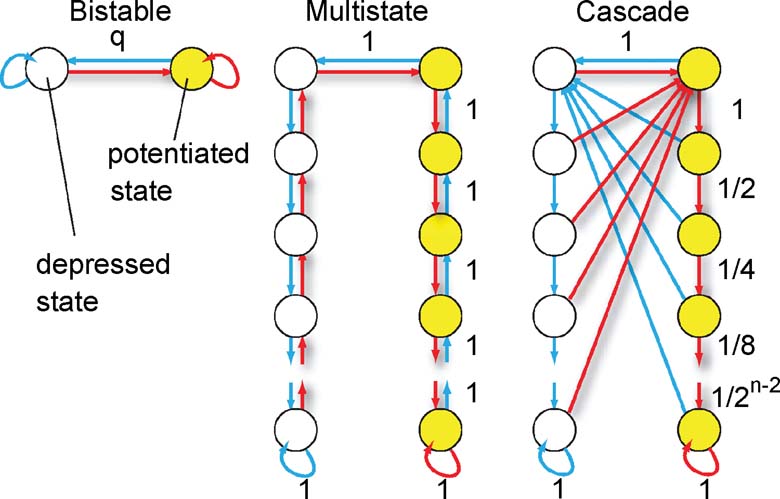
Figure 1. Schemes of synaptic states for the bistable, multistate, and cascade models. Every circle denotes a synaptic state. Yellow circles correspond to a potentiated synapse, that is, a synapse with an elevated efficacy. Empty circles correspond to depressed synapses. The arrows represent the possible transitions between states. Red arrows are the transitions in the case the neural activity tends to potentiate the synapse. Blue arrows correspond to synaptic depressions. Some of the learning rates are reported with black numbers. They are q for the bistable model, always one for the multistate model, and they decrease as 1∕2k for the cascade model, where k is the metaplastic level (number of states from the top of the cascade). The states at the bottom are the most resistant to plasticity, whereas those at the top are the most plastic ones.
The bistable model has an initial that scales like  (Amit and Fusi, 1994
) when the patterns have sparseness f. The signal decays with time as exp(−rtqf2), where rt is the number of shown memories at time t with rate r. The memory lifetime can be extended arbitrarily by reducing q, at the price of reducing the initial by the same factor (Amit and Fusi, 1992
; Amit and Fusi, 1994
; Tsodyks, 1990
). Small qs correspond to slow learning and long memory lifetimes, whereas qs that are close to 1 correspond to fast learning and fast forgetting. The multistate synapses show a similar behavior, with the only difference that with n states, their initial is reduced by a 1∕n factor whereas the memory lifetimes are extended by a 1∕n2 factor (Amit and Fusi, 1994
). The bistable model, the simplest, is also very robust to unbalanced potentiation and depression when compared to the multistate model (Fusi and Abbott, 2007
). Finally, the cascade model has the advantages of long memory retention, as in the case of a bistable synapse with small q, and fast learning, corresponding to a large q. Indeed on the one side, its initial scales like the bistable model for q = 1 multiplied by a factor 1∕n. The decay of the memory trace is not exponential but it follows a power law for a long time, proportional to 2n, and then it goes down exponentially.
(Amit and Fusi, 1994
) when the patterns have sparseness f. The signal decays with time as exp(−rtqf2), where rt is the number of shown memories at time t with rate r. The memory lifetime can be extended arbitrarily by reducing q, at the price of reducing the initial by the same factor (Amit and Fusi, 1992
; Amit and Fusi, 1994
; Tsodyks, 1990
). Small qs correspond to slow learning and long memory lifetimes, whereas qs that are close to 1 correspond to fast learning and fast forgetting. The multistate synapses show a similar behavior, with the only difference that with n states, their initial is reduced by a 1∕n factor whereas the memory lifetimes are extended by a 1∕n2 factor (Amit and Fusi, 1994
). The bistable model, the simplest, is also very robust to unbalanced potentiation and depression when compared to the multistate model (Fusi and Abbott, 2007
). Finally, the cascade model has the advantages of long memory retention, as in the case of a bistable synapse with small q, and fast learning, corresponding to a large q. Indeed on the one side, its initial scales like the bistable model for q = 1 multiplied by a factor 1∕n. The decay of the memory trace is not exponential but it follows a power law for a long time, proportional to 2n, and then it goes down exponentially.
Synaptic state occupancies
In order to study the decay of the memory trace, we evaluate the as a function of time. Hence, we need to compute the first and second order terms of the total synaptic current h for all pairs of pre- and postsynaptic activities imposed by the pattern generating the tracked memory (Amit and Fusi, 1994
). We use a “mean field” approach in which we compute the conditional synaptic distributions at every time step. For every pair of pre- and postsynaptic activities, we compute the probability  of occupying a given state l, given that the pre- and postsynaptic activities are x and y during the creation of the tracked memory. In the general case, the probability
  , at time t + 1∕r, after a new memory has been stored, of occupying state l = 1, 2,…,n can be written as:
where Mlm is the probability of making a transition from state m to state l. We assume that the memories stored after the tracked one are created by patterns which are random and not correlated to the values of x and y. Mlm generally depends on the learning rule, on the synaptic model, and on the statistics of the neural representations of the memories (i.e., f).
For all the models studied here, and more generally for any realistic model with a finite number of states, there exists an equilibrium distribution which corresponds to the state reached after the storage of a large number of memories created by random patterns. The equilibrium distribution is uniform for both R1 and R2 as the total probabilities of potentiating and depressing a synapse are balanced. As the memory we track is not a special memory, but it can be created by any event in the past, we start from the equilibrium distribution and we then modify the conditional synaptic distributions. For example, for the bistable model, we have only two states, the synapse can be either depressed (state 0) or potentiated (state 1). We assume that for example the imposed pre- and post-synaptic activities are active (x = y = active). If the learning rule is R1, the only permitted transition is potentiation with probability q+. Therefore, if we start from the equilibrium distribution F(t = 0) = [F0(t = 0), F1(t = 0)] = [1∕2, 1∕2] at time 0, the distribution at time 1∕r (i.e., after the tracked memory is stored) will be:  , where Q+,+ is a transition probability matrix that contains the initial conditions x = y = +, that is, active. Bold letters represent vectors. The distribution F after the next memories are stored can be calculated simply using the Markov chain rule, by having the next iteration starting from the previous one, but replacing matrix Q+,+ with the general transition matrix M (containing the elements Mlm), since the next patterns will stochastically activate x and y (see Appendix A.2). More generally, with any given initial conditions for the pre- and postsynaptic activity, the synaptic distribution can be computed at any time using the above time difference stochastic equation. For more details about the calculation of F, Q, and M see Appendix A.2.
Results
Memory retrieval in the presence of correlated noise
The ability to retrieve a memory depends on the number of synapses, on the statistics of the neural patterns of activities creating the memories, and on the synaptic dynamics. In order to estimate the memory performance as a function of these different factors, we consider statistically independent random patterns of activities. Every pattern creates a memory which later might be partially or completely overwritten by other memories. In order to establish whether a memory can be retrieved or not, we estimated a memory signal which is defined as a difference between the normalized total synaptic current of the neurons that should be active and the normalized current of the neurons which should be inactive (see Section “Materials and Methods” for more details). Such a current varies from neuron to neuron, even when we consider only neurons that should be active. This variability is due to the fact that the patterns generating the memories are random and different neurons in general see different input patterns. The average value of the memory signal is normalized in such a way that it does not depend on the average number, C, of plastic synapses on the dendritic tree of a single neuron. The width of the distribution can be estimated by computing the noise, which is given by the standard deviation of the total synaptic current across different neurons. Two components constitute the squared noise. The first one scales as 1∕C, that is what we would have in the case of completely independent synapses. The second component does not depend on C, and it is due to the correlations between synapses on the same dendritic tree. To understand the origin of the second component, consider rule R1 for updating the synapses; when the presynaptic neuron is active, the synapse is modified. The direction of the change depends on the postsynaptic activity; potentiation occurs for an active postsynaptic neuron, depression otherwise. The synapses on the same dendritic tree are clearly correlated even in the case of uncorrelated random patterns of neural activity; if a synapse is potentiated, all the other synapses will be either potentiated or left unchanged, because they share the same postsynaptic activity. Had the synaptic modifications been independent, the other synapses could also undergo depression. The existence of these correlations can completely disrupt the ability to retrieve memories. Indeed, in case of uncorrelated noise, the would scale like  , which would always allow memory retrieval, provided that the number of synapses is sufficiently large. For correlated noise, there would be no improvement in the memory lifetime when the number of synapses increases, making the storage resources of a large number of synapses completely useless. This problem was noticed already in Amit and Fusi (1994)
for a bistable synaptic model, and it was solved by the authors by assuming that the patterns of activity generating the memories are sparse. Indeed, for R1, the uncorrelated part of the squared noise does not depend on the sparseness, but the correlated part decays linearly with f. Notice that the uncorrelated part of the noise does not depend on time, whereas the correlated part is modulated by the storage of other memories (see Figure 2
(a)).
, which would always allow memory retrieval, provided that the number of synapses is sufficiently large. For correlated noise, there would be no improvement in the memory lifetime when the number of synapses increases, making the storage resources of a large number of synapses completely useless. This problem was noticed already in Amit and Fusi (1994)
for a bistable synaptic model, and it was solved by the authors by assuming that the patterns of activity generating the memories are sparse. Indeed, for R1, the uncorrelated part of the squared noise does not depend on the sparseness, but the correlated part decays linearly with f. Notice that the uncorrelated part of the noise does not depend on time, whereas the correlated part is modulated by the storage of other memories (see Figure 2
(a)).
Is it possible to eliminate the correlated part of the noise without recurring to sparseness? We can actually modify the synaptic dynamics R1 to strongly reduce the effects of the correlated part of the noise. Following Tsodyks and Feigelman (1988) , we balance the transitions between synaptic states in such a way that there are no correlations between synapses when the neural patterns of activities are random and uncorrelated. We assume that the synapse is potentiated also when the pre- and the postsynaptic neurons are inactive, depression occurs otherwise. We tune the learning rates in such a way that when a synapse potentiates, the other synapses on the same dendritic tree have the same probability of potentiating and depressing, as in the uncorrelated case. Indeed, now a synapse can potentiate every time the pre- and postsynaptic activities are the same. The probability that a different synapse on the same dendritic tree also potentiates is now independent of the direction of synaptic modification of the first synapse and it is determined by the presynaptic activity, which is random and uncorrelated, regardless of the postsynaptic activity. For such a rule, the squared noise for the equilibrium distribution does not depend on f (see Figure 2 (b)). The correlated part of the noise is always strongly reduced when compared to that of R1, it peaks at a certain time, and then it becomes small for large t.
The equilibrium noise for R1 and the maximal noise for R2 are plotted in Figure 2
(c) as a function of f. Notice that there is a maximum in the correlated noise for both rules. The correlated part of the noise at equilibrium for R2 is negligible and the total noise decreases as the uncorrelated term like  (see Figure 2
(d)). In what follows, we will study more complex models of synaptic plasticity but we will always use the decorrelating R2. This allows also a great simplification of the analysis as we can neglect the correlated part of the noise.
(see Figure 2
(d)). In what follows, we will study more complex models of synaptic plasticity but we will always use the decorrelating R2. This allows also a great simplification of the analysis as we can neglect the correlated part of the noise.
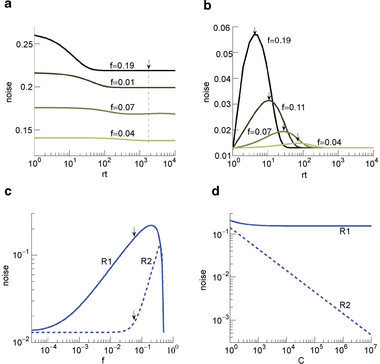
Figure 2. Noise  the case of the bistable model. (a) Noise for C = 104 for R1 for four different levels of sparseness: f = 0.19, 0.11, 0.07, 0.04, from darker to lighter lines. (b) Noise for C = 104 for R2 for the same fs reported in (a). (c) Noise for R1 (solid) and R2 (dashed) as a function of f, obtained taking the points indicated by the arrows in Figures 2
(a) and 2
(b) for large C. (d) Noise for R1 (solid) and R2 (dashed) as a function of C(f = 0.055) for the points indicated by the arrows in Figure 2
(c).
the case of the bistable model. (a) Noise for C = 104 for R1 for four different levels of sparseness: f = 0.19, 0.11, 0.07, 0.04, from darker to lighter lines. (b) Noise for C = 104 for R2 for the same fs reported in (a). (c) Noise for R1 (solid) and R2 (dashed) as a function of f, obtained taking the points indicated by the arrows in Figures 2
(a) and 2
(b) for large C. (d) Noise for R1 (solid) and R2 (dashed) as a function of C(f = 0.055) for the points indicated by the arrows in Figure 2
(c).
Memory retrieval performed by single neurons
The memory trace for cascade models decays as a power law over a time interval which increases exponentially with the number of levels of the cascade (Fusi et al., 2005
). After that time, the decay becomes exponential and hence significantly more rapid. If we require that the is larger than a certain threshold, then the number of memories which can be retrieved grows as a power law of the number of synapses C. This scaling compares favorably to the logarithmic dependence on C of non-cascade models. We now analyze how the memory performance of cascade models is affected by the sparseness of neural patterns of activities which create the memories. In Figure 3
(a), we show the of a cascade model as a function of time for three different levels of sparseness and for C = 10 000, n = 10. The curves are plotted in a log-log scale, thus straight lines represent power laws. As f decreases (lighter lines), the initial also decreases, but the memory lifetime slightly increases. The curves can be fitted by the following function:
The function has been determined as in Fusi et al., (2005)
by simple considerations based on the scaling properties of the signal and the noise. The initial (obtainable by setting t = 0) has been determined analytically. The decay is due to two factors. The first is a power law ∼1∕t, and the second is an exponential term which dominates when t is larger than the longest time constant of the cascade. The power of the first term (−1), estimated by fitting the formula to the mean field results, is slightly different from the one estimated in Fusi et al., (2005)
(−3∕4) as it has been determined to describe the decay in a different range. The numerical coefficients also result from a fit and they have been expressed as fractions for readability. All times are scaled by a factor f2. This is simply because in R2 the probability of modifying a synapse is proportional to f2. It is as if only a fraction f2 of all memories actually modify a specific synapse.
For the range  , n = [5,15] and f = [10−4,0.5], the goodness of the fit is 0.97 and it is assessed by taking the relative error
  for each point and then calculating the quantity
  where
where  ; the closer the value is to one the better the fit is (similarly to the coefficient of determination R-squared in statistics).
The initial (obtainable for t = 0) contains all the dependence on C, which comes from the dependence of the uncorrelated part of the noise. Moreover, it is inversely proportional to the number n of levels of the cascade because at the equilibrium distribution all metaplastic states are equally occupied (see Fusi et al., (2005)
for more details). Finally, the initial signal depends linearly on f. The explanation is simple: consider a postsynaptic neuron which should be active in response to the input when a memory is retrieved. All synapses connecting active presynaptic neurons (which are a fraction f of all neurons) are potentiated with probability 1, and all synapses connecting inactive presynaptic neurons (fraction 1 − f) are modified with probability f. Hence, the total contribution is proportional to f if higher order terms are neglected.
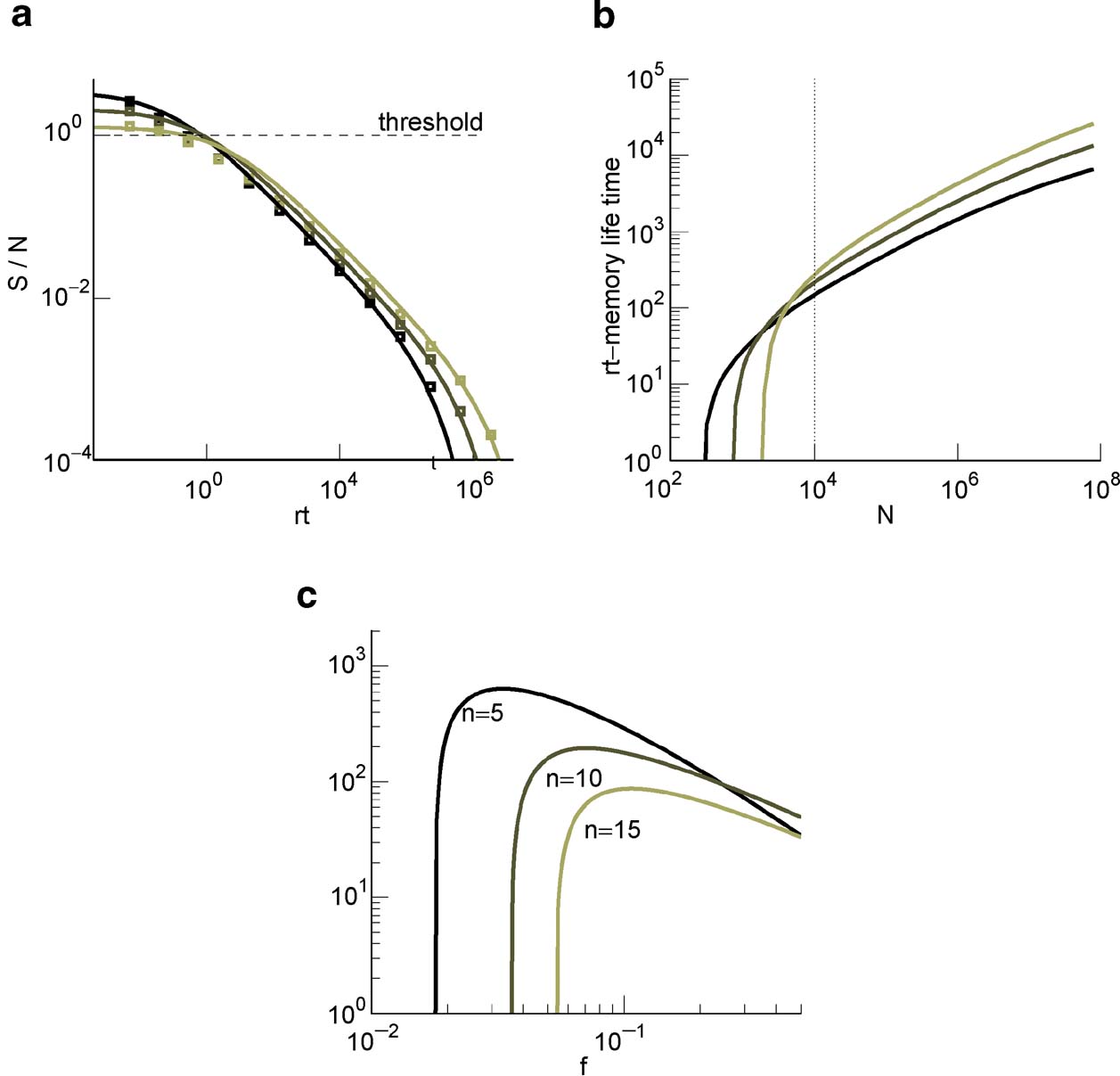
Figure 3. (a) of cascade (solid curves are the fits of Equation (2) and the squares are obtained from the mean-field calculation) with n = 10 at N = 104 and decreasing values of f = 0.19, 0.11, 0.07 (lighter lines). (b) rt at which the ratio of Equation (2) goes below 1. Same f s as in (a). The dotted line corresponds to the 104 synapses. (c) Memory lifetime as a function of f for N = 104 and for n = 5, 10, 15 (light lines correspond to increasing values of n).
The memory lifetime is estimated as explained in Section “Materials and Methods,” by requiring that the is larger than a particular threshold (we allow an average error of 15%). The results are plotted in Figure 3
(b). Notice that as it is clear from Figure 3
(a), for C = 10 000 the initial is very close to the critical threshold, and most of the power law decay occurs in a region in which memories cannot be retrieved. Such a behavior depends on the number of levels n of the cascade, as it will also be discussed in the next section, and on the number of synapses C. In Figure 3
(c), we plotted the memory lifetime as a function of sparseness f for three values of n. The best performance is obtained for the smallest n, because for a single neuron with a relatively small number of synapses (C = 10 000) the maximum memory lifetimes are anyway small and any additional complexity would not help to extend the memory. Notice that for all three curves, there is an optimal f = fM and a minimal value f = f0 below which the memories cannot be retrieved. The nonmonotonic behavior comes from the fact that just above f0 the number of storable memories increases with f, reflecting the dependence of the initial on the sparseness. Then it decreases because the memory lifetime is inversely proportional to the average number of modified synapses, which scales like f2.
Memories can be retrieved only if sparseness is limited
Memory lifetimes are inversely proportional to f2, and hence sparse stimuli mean longer memories. However, f cannot be arbitrarily reduced as single neurons can retrieve memories only if the initial is above a certain value. If it is not possible to retrieve a memory immediately after it has been stored, when it is most vivid, then it is impossible to retrieve it after other memories partially or completely overwrote it. The initial is proportional to  (see Equation (2)) and hence it decreases linearly with f when the stimuli become sparser.
In order to retrieve memories, the initial must be larger than a certain threshold, which in turn depends on the average number of errors produced during retrieval. For simplicity, we consider a threshold 1, which corresponds to errors in response to 15% of the input patterns. As we noticed in the previous section, for any given pair of C and n, there is a minimal f = f0 below which it is not possible to retrieve any memory:

The smallest f is constrained by the complexity of the synapse, represented by n, and by the number of synapses C which are directly accessible by each neuron.
Complexity reduces the initial
The initial decreases with sparseness, but it is also reduced when complexity increases (larger n). This is a general property of a large class of metaplastic synapses and it is an obvious consequence of the existence of multiple synaptic states. Indeed, if all the states are visited with a non-zero probability, the synapse will spend only a fraction of its time roughly proportional to 1/n in the most plastic states, which are those that contribute the most to the initial . How does the memory lifetime of single neurons scale with complexity and f? If the synapse operates in the power law regime (rt⪡2n−2/f2), the best memory performance is obtained for fM = 2f0. The dependence of memory lifetime on f and on n is illustrated in Figure 3
(c) and its maximum is given by

Notice that such a memory lifetime decreases rapidly with the number n of metaplastic states. So what would be the advantage of using a complex synaptic model with a large n?
Memory retention in synapses across multiple neurons
The need for complexity comes from various considerations about the memory capacity of multiple neurons. When we combine together the information stored in synapses of different dendritic trees, we cannot determine the number of retrievable memories without specifying the architecture of the network and the neural dynamics. However, we can estimate an upper bound of the memory lifetime by considering the point of view of an “ideal observer,” as in Fusi et al., (2005) , who has a direct access to the set of all synapses. Such an observer can determine whether a memory is retained by measuring the correlation between the current set of synaptic efficacies and the pattern of synaptic modifications which created the tracked memory. Indeed, the pattern of synaptic modifications is determined by the neural activities and hence it contains all the storable information about the particular stimulus or event which created the memory. If the current synaptic efficacies are not correlated to such a pattern, then the memory is forgotten. The correlation is highest immediately after the tracked memory is stored, and then it is degraded by other experiences, which also impose patterns of synaptic modifications. We assume that these patterns are random and uncorrelated. The decorrelating learning rule would actually guarantee that the synaptic modifications are statistically independent when we assume that the neural representations generating the memories are also random, uncorrelated, and arbitrarily sparse. Notice that this is true also when two postsynaptic neurons share a certain number of inputs. Indeed, the synapses sharing the same presynaptic neuron are not correlated for the same reason that two synapses on the same dendritic tree are uncorrelated (see Section “Memory Retrieval in the Presence of Correlated Noise”).
Following Fusi et al., (2005)
, we now estimate quantitatively the maximum number of memories which can be retained when N statistically independent synapses are considered. We divide the synapses into two groups, those which are potentiated and those which are depressed when the tracked memory is created. We define the memory signal as the average difference between the number of synapses in the two groups and the noise as its standard deviation. Notice that we assume that the synapses are statistically independent, so there are no correlations between different synapses. Not surprisingly, the for memory retention of synapses on multiple neurons decays as the for memory retrieval of single neurons in the case of uncorrelated noise. The only difference is that instead of the number of synapses C on the dendritic tree of a single neuron, we now have N, which is the total number of synapses of multiple neurons. The expressions are the same because memory retrieval in single neurons is equivalent to read out the correlations between the synaptic efficacies and the input pattern which was imposed when the tracked memory was created. The main difference is that in the case of single neuron memory retrieval the synapses share the same postsynaptic neuron and hence they can be correlated. In the case of memory retention in multiple neurons, we totally ignore the architecture of the network and we assume that the synapses are completely independent. The for memory retention can also be computed with small modifications of the mean field approach introduced in Fusi et al., (2005)
, and it can be fitted by the following function:
If rt⪡2n−2/f2, then
The tracked memory is retained if this is larger than some threshold, which we assume for simplicity to be unitary. Then we have approximately

Relation between synaptic complexity and sparseness
As discussed in the previous section, we do not know how to retrieve the information when it is distributed across different neurons. However, we can safely assume that f is larger than f0, the minimal value of f which would allow each single neuron to retrieve the memories stored in its C synapses (see also Section “Discussion”). Such a condition guarantees that the initial is larger than 1, and imposes a lower bound on f. It is important to keep in mind that every neuron sees only C synapses, and not all the N synapses which are available to multiple neurons. At f = f0, the memory lifetime would be exactly zero, so f should be larger than f0. In what follows, we assume that f is tuned in such a way that every single neuron has the best memory performance (f = fM). As fM = 2f0, we would obtain the same scaling properties if we do the analysis with f0 instead of fM.
Let us consider first the case of lowest complexity n = 2, which would allow us to choose the sparsest stimuli. In such a case, we basically do not have a cascade model, the decay is entirely dominated by the exponential term, and the memories are retained as long as approximately  . If we choose the lowest f which would still allow single neurons to do retrieval, we obtain

This way we would use very inefficiently the memory resources provided by multiple neurons given that the memory lifetime grows only as the logarithm of the total number of synapses. We can actually do much better if we increase the synaptic complexity. We assume that  and we get that the maximal retention time of a memory stored in N synapses is given by Equation (4) and it is approximately

In order to derive this expression, we neglected the 1 at the denominator of Equation (4). Such an approximation is valid as long as N⪢C∕4, which is certainly true for all the cases that we will analyze. The upper bound on rt is correct as long as  , which would correspond to the condition that the cascade model operates in the power law regime. Notice that now the maximal number of memories increases with the square root of the total number of synapses, which can be a very large number, even when a single cortical column is considered (N ∼ 108–109). If M is the total number of neurons, and we assume that each neuron has C synapses, then N = CM, and

Such a favorable scaling is valid only if the synapses operate in the power law regime, which implies

This inequality is obtained by replacing fM = 2f0 in the expression . One of the consequences of such an inequality is that the synapse should have a number n of metaplastic states that grows approximately as the logarithm of the maximal memory lifetime. In other words, the complexity of the synaptic dynamics should increase in order to harness the storage resources provided by the N synapses. As n increases, the initial decreases. If C is set to a fixed value, then the only way to still guarantee the ability to retrieve information at the level of a single neuron is to reduce the level of sparseness by increasing f. This conclusion is illustrated in Figure 4
(a) where we plotted the minimal and the optimal f (f0 and fM, respectively) as a function of the maximal memory lifetime which can be obtained for statistically independent synapses. Given a desired memory lifetime rt, we first computed the number n of necessary metaplastic states by solving Equation (5), with C = 1000 (red line) and C = 10 000 (blue line), see Figure 4
(b). Given the resulting n(rt), we then computed and plotted  and fM = 2f0 in Figure 4
(a). f0 is a function of n and, again, C = 10 000 and C = 1000. We conclude that if large memory lifetimes are needed, then the neural representations of the memories cannot be too sparse, otherwise they cannot be retrieved. For the range of Cs that we considered (103–104), f is constrained to be of the order of 10−2–10−1. The corresponding number of storable memories ranges from 104 for the sparsest representations (f ∼ 0.01) observed in the medial temporal lobe (Barnes et al., 1990
; Jung and McNaughton, 1993
; Quiroga et al., 2005
), to 107 for f ∼ 0.1–0.2 similar to the sparseness observed in inferotemporal and prefrontal cortices (Rolls and Tovee, 1995
; Sato et al., 2007
). The memory lifetimes depend on the rate r of creation of memories. If, for example, r = 0.1 s, then memory lifetimes for f ∼ 0.01–0.05 would be in the range of one or a few days, whereas for f ∼ 0.1–0.2, they would be of the order of 3–4 years.
and fM = 2f0 in Figure 4
(a). f0 is a function of n and, again, C = 10 000 and C = 1000. We conclude that if large memory lifetimes are needed, then the neural representations of the memories cannot be too sparse, otherwise they cannot be retrieved. For the range of Cs that we considered (103–104), f is constrained to be of the order of 10−2–10−1. The corresponding number of storable memories ranges from 104 for the sparsest representations (f ∼ 0.01) observed in the medial temporal lobe (Barnes et al., 1990
; Jung and McNaughton, 1993
; Quiroga et al., 2005
), to 107 for f ∼ 0.1–0.2 similar to the sparseness observed in inferotemporal and prefrontal cortices (Rolls and Tovee, 1995
; Sato et al., 2007
). The memory lifetimes depend on the rate r of creation of memories. If, for example, r = 0.1 s, then memory lifetimes for f ∼ 0.01–0.05 would be in the range of one or a few days, whereas for f ∼ 0.1–0.2, they would be of the order of 3–4 years.
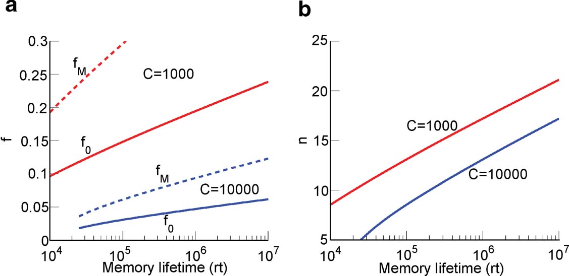
Figure 4. Relation between sparseness and memory lifetime. (a) The minimal and the optimal sparseness (f0 and fM, respectively) are plotted against a desired memory lifetime for C = 1000 (red) and C = 10 000 (blue). As memory lifetime increases, the number of needed metaplastic states n also increases (b), and this imposes an upper bound on the sparseness (a lower bound on f).
Memory retrieval with alternative models
The next question we ask is whether it would be possible to obtain a similar memory performance for M neurons with other complex synaptic models with the same number of states. In principle, we could rely solely on sparseness to extend the memory lifetime, without recurring to metaplasticity. In practice, the non-cascade models have in general a logarithmic, very weak dependence of memory lifetime on M which would require a sparseness which goes to zero with M and hence prohibitively low values of f. Interestingly, the considerations about the relation between synaptic complexity and sparseness are still valid for a large class of efficient n state synaptic models.
We analyzed the multistate model as we did for the cascade model. The can be nicely fitted by

The formula can be easily derived from the analysis of Fusi and Abbott (2007) and the numerical coefficient 9∕5 has been determined by fitting the formula to the mean field estimates (goodness of fit 0.99). The of the cascade and of the multistate model are plotted in Figure 5
for C = 10 000 and for f = 0.19. Notice that for such a relatively small number of synapses, there is a wide interval of time in which the multistate model outperforms the cascade model with the same number of states. This is again another expression of the fact that complexity is required for storing information in a large number of synapses, when multiple neurons are considered, and it might appear to be deleterious when a single neuron with a relatively small number of synapses is considered.
For the multistate model, there is also a maximum memory lifetime for a certain f, as already noticed in Leibold and Kempter (2007) . Such a maximum is approximately at fM = 8f0∕5 where f0 is the minimal f which allows retrieval and it depends on n and C similarly to the f0 of the cascade model:

The memory lifetime at the maximum is simply C∕100 and surprisingly it does not depend on n. When M neurons are considered, then the upper bound of the memory capacity is approximately

The log M dependence on the number of neurons should be compared to the  dependence of the cascade model. The reduction due to n2 of the memory lifetime of the cascade model seems to be a small price to be paid in comparison to the advantage of a dependence. Such an advantage becomes particularly relevant when the total number of synapses is large.
The upper bound of the memory capacity of the two models for an increasing number of statistically independent synapses N is plotted in Figures 6 (a) and 6 (b) for n = 10, 15, 15 when f = 0.1. In both cases, the cascade model performs better than the multistate for N > 106 when n = 10 and N > 108 when n = 15. Notice that in a single cortical column, we probably already have N > 109.
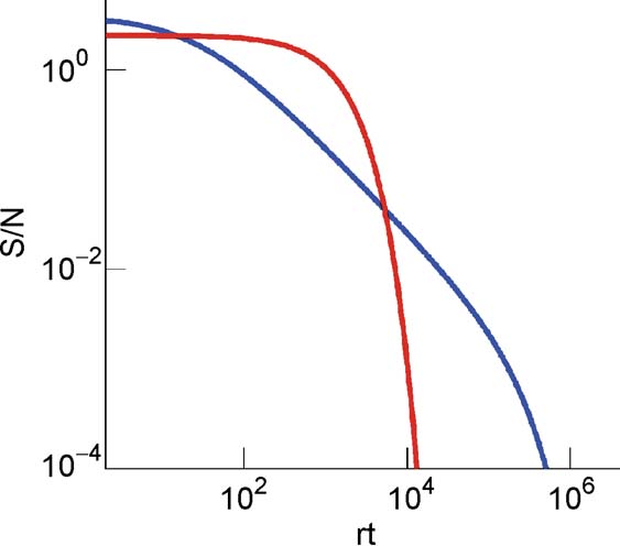
Figure 5. of the cascade (blue) and of the multistate (red) model for C = 104 and for f = 0.19 as a function of the number of storedmemories rt.
An extensive comparison of the two models is made by examining the contour plot of Figures 6
(c) and 6
(d) where the ratio between the capacity of the cascade over the multistate model is plotted for N = [102,1012] and f = [10−4,0.5] in log scale for both N and f. The black-shaded area corresponds to the region where the multistate model has zero capacity because the initial is below the critical threshold. The lines are cutting the (f, N) plane along the curve  , where α is a coefficient that controls the position of the level lines. This fit is good for f < 0.1 while for bigger values of f the lines tend to curve slightly to the left of the graph. This is because of the nonmonotonic behavior of the noise component as we approach 0.5 (see Figure 2
(c) where for f ∼ 0.3–0.5 noise increases).
, where α is a coefficient that controls the position of the level lines. This fit is good for f < 0.1 while for bigger values of f the lines tend to curve slightly to the left of the graph. This is because of the nonmonotonic behavior of the noise component as we approach 0.5 (see Figure 2
(c) where for f ∼ 0.3–0.5 noise increases).
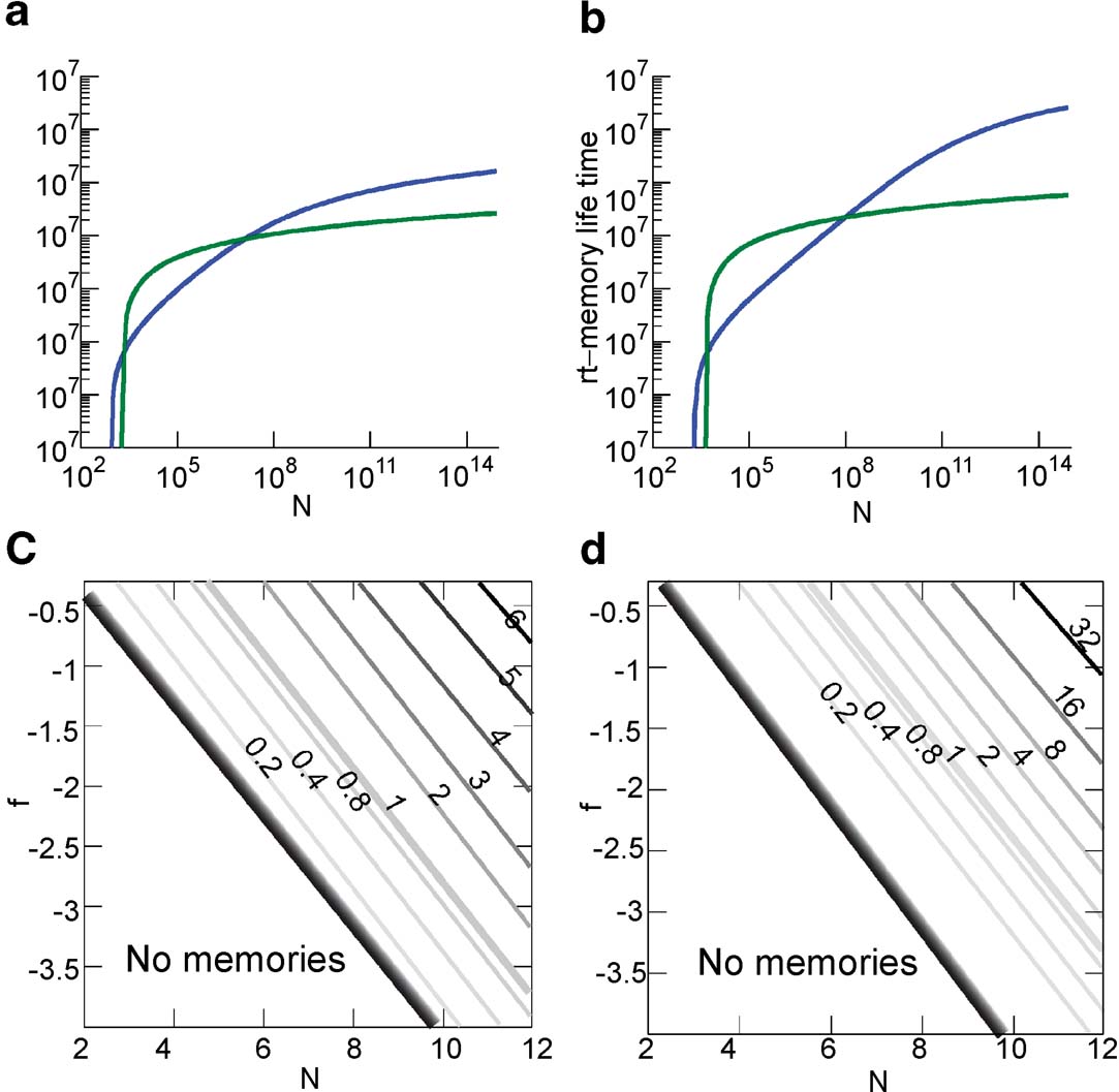
Figure 6. Comparison of the memory lifetime of the cascade (in blue) and the multistate model (in green) for f = 0.1 (a) for n = 10 (b) and n = 15. (c) Ratio of the memory lifetime of cascade over multistate model as a function of N and f for n = 10 (N and f are in Log10 base). The graded black area corresponds to the range in which the cascade has much higher memory capacity. (d) The same as above for n = 15.
Discussion
We showed that complex cascade models of synapses can memorize and retrieve a large number of random uncorrelated patterns. Our analysis extends the results of Fusi et al., (2005) from populations of independent synapses to single neurons where the synapses on the same dendritic tree can generate harmful correlations, also in the case of memories created by random uncorrelated patterns of activities. These correlations are exactly zero for random uncorrelated patterns in which on average half of the neurons are activated, or negligible in the case of extremely sparse patterns. However, for the levels of sparseness observed in the brain, they might disrupt the ability to retrieve memories because the correlated part of the noise grows as fast as the memory signal when the number of synapses increases. We introduced a learning rule which allows to cancel the correlations given that the average sparseness f of the patterns is known. Indeed, the learning rates for both potentiation and depression must depend on f in order to eliminate the correlations. Such information might be available to single synapses by reading out some global signal generated by some unknown mechanism operating on a longer timescale. Such a mechanism might be involved in the global processes of protein synthesis which, in turn, would permit the expression of long-term synaptic modifications.
The neural system that we analyzed is highly simplified and the neurons are only either active or inactive. We believe that such a simple model captures many important features of the memory performance of more realistic models of long-term synaptic dynamics, and we know that learning prescriptions similar to ours can be implemented with detailed, biologically realistic synaptic dynamics (Fusi et al., 2000 ; Mongillo et al., 2005 ). However, it does not incorporate the complexity of the detailed biochemical processes that lead to long-term synaptic modifications and this might generate misleading interpretations. For example, the decorrelating learning rule requires that the synapses are potentiated when both the pre- and the postsynaptic neurons are inactive, though the modifications should be consolidated with a small probability (∼f2). This does not necessarily imply that the synapses are continuously modified at the same rate as they are updated when the neurons are stimulated. Neuromodulators like dopamine are known to greatly modulate the learning rates (Reynolds and Wickens, 2002 ) and they might activate the process which creates a memory only when a relevant event occurs. Moreover, many protocols to induce long-term synaptic modifications like spike-timing-dependent plasticity require very specific patterns of pre- and postsynaptic spikes, and our two neural states can simply correspond to some specific trains of spikes which do not occur during spontaneous activity. On the other hand, it might also be that synapses are actually modified by spontaneous activity, as already observed in Zhou et al., (2003) , and our learning rule would be compatible with such a scenario as the learning rate in the case of inactive neurons is supposed to be significantly smaller than in the other cases.
After the introduction of a decorrelating learning rule, we analyzed the relation between the complexity of the mechanisms responsible for memory preservation and the sparseness of the neural patterns of activity which create the memory. The initial memory trace corresponds to a vivid memory which then fades away as new memories are stored. If such a trace is not sufficiently strong, then it is not possible even to store a memory. The strength of the initial memory trace is proportional to f and to the square root of the connectivity C and inversely proportional to the number of metaplastic states n. If the latter, representing a measure of the complexity of the synaptic dynamics, increases to extend the memory lifetime and C is kept constant, then f has also to increase by the same amount. As the advantage due to increased complexity is huge when one considers a large number of synapses, then longer memory lifetimes would require less sparse neural representations.
This result is based on the assumption that every neuron singularly has to be able to retrieve as many memories as possible, or at least it should be able to retrieve at least one memory. We do not know how to estimate the number of patterns which can be retrieved by a large network of connected neurons because this would require to specify the neural dynamics of highly interconnected networks of neurons and of multimodular networks. We know that it is very difficult to study large networks of neurons and that the performance can be surprisingly poor when neural cells are interacting at a multimodular level (O'Kane and Treves, 1992 ). With these premises, we think that a good memory performance could be achieved when we require that every neuron retrieves the maximum patterns that it can, or, at least, when we demand that every neuron can retrieve more than one pattern without errors. In principle, it might be possible to build a network in which every neuron makes a large number of mistakes and then these errors are corrected by some complicated interaction with other seemingly failing neurons. However, it is probably easier to assume that single neurons operate in a regime in which they can retrieve patterns on the basis of the memory signal that we defined. Interestingly, if we make this assumption, we then constrain the sparseness of the neural representations in a range which is very close to the sparseness observed in the brain (Asaad et al., 1998 ; Barnes et al., 1990 ; Jung and McNaughton, 1993 ; Rolls and Tovee, 1995 ; Sato et al., 2007 ).
Notice that the constraint on sparseness that we derived depends on the requirement that synapses on multiple neurons need to be complex (i.e., have a large number of states) in order to store in their synapses an extensive number of memories. Our estimates of the maximal number of retainable memories are based on the assumptions that an ideal observer can read out all synapses simultaneously and that the synaptic modifications are statistically independent. The first hypothesis makes our estimate an upper bound, and the second is discussed below in Subsection “Correlated Neural Representations of Memories.” However, it is important to notice that the estimate does not depend on the particular neural dynamics, on the architecture of the network, and on the way the neurons interact. We essentially estimate the number of retainable memories by assuming that the different synapses are like independent bits of a computer memory. If the memory trace is not stored in the synapses, then there is no way that the memory can be retained and, of course, a fortiori, the memory cannot be retrieved. In this sense, our estimate is a strict upper bound for the memory capacity.
Our study predicts that across different brain areas, like inferotemporal cortex versus medial temporal lobe, longer lifespan of storied memories should be correlated with a larger number of metaplastic synaptic states, and correspondingly neurons are expected to respond to a larger number of stimuli.
Relation to previous works on sparseness
Sparseness has been shown to extend the memory lifetime in many publications (Treves, 1990 ; Tsodyks and Feigelman, 1988 ) and to play a particularly important role in the case of bounded synapses (Amit and Fusi, 1994 ; Leibold and Kempter, 2007 ). The conclusions of these works seem to be in contradiction with our result that sparseness should be reduced when long memory lifetimes are required. However, the contradiction is only apparent because we also believe that sparseness greatly contributes to extend memory lifetimes in case of single neurons, or in the case of multiple neurons when different neurons store on their dendritic tree the same input pattern of neural activity (e.g., in the case of recurrent neural networks in which attractors (Amit and Fusi, 1994 ; Treves, 1990 ; Tsodyks and Feigelman, 1988 ) or sequences of patterns (Leibold and Kempter, 2007 ) are stored). However, in all these studies the authors did not analyze the memory performance of a network of neurons which is larger than the local one considered. We showed that in such a case sparseness cannot be the only solution to the memory capacity problem as each neuron still sees a limited number of synapses when large networks are considered, and hence the sparseness cannot be arbitrarily reduced. It is particularly interesting to discuss the cases of Amit and Fusi (1994) and Leibold and Kempter (2007) . In both papers, the authors consider realistic binary synapses, and they show that the memory lifetime scales like f−2log(fC). If the sparseness increases with C, then the memory lifetime increases with a very favorable scaling because of the f−2 factor in front of the logarithm. However, the initial memory trace is also reduced and in order to be still above the threshold of retrievability, f > 1∕C. As consequence, the upper bound of the number of retainable memories in multiple neurons would scale like C2 and it would depend only logarithmically on the total number of neurons M. Notice that the f−2 factor cannot be used to obtain an M2 dependence on the total number of neurons as f cannot become arbitrarily small (f should be larger than 1∕C) as required by f ∼ 1∕M. Moreover, the scaling properties of neurons encoding sparse representations are correct only if the correlations between synapses are negligible (Amit and Fusi, 1994 ).
In the case of the complex cascade models, the number of memories increases approximately as  and it decreases with complexity. As n increases very slowly with the longest memories lifetimes, it is clear that there is always an M such that the performance of the cascade synapses is better than a network which relies only on sparseness. However, such a number can be very large, even larger than the total number of neurons in the brain. If this is the case, then complexity has only a negative effect on memory lifetimes (Leibold and Kempter, 2007
).
and it decreases with complexity. As n increases very slowly with the longest memories lifetimes, it is clear that there is always an M such that the performance of the cascade synapses is better than a network which relies only on sparseness. However, such a number can be very large, even larger than the total number of neurons in the brain. If this is the case, then complexity has only a negative effect on memory lifetimes (Leibold and Kempter, 2007
).
We showed that for realistic parameters this is not what happens and that cascade models perform better already for the number of neurons which are in a single column. Leibold and Kempter (2007)
seem to actually reach the opposite conclusion. One of the explanations of this apparent contradiction is that they assumed that inactive neurons have exactly a zero contribution to the noise of the memory signal. In their case, the noise is then proportional to f. As soon as some noise is introduced in the inactive neurons (e.g., spontaneous activity), the scenario drastically changes. In particular, when the standard deviation of the noise is larger than  , where ξ+ is the mean activity of active neurons, then the dominant term of the total noise of the memory trace does not depend on f, and the minimal f which would allow single neuron retrieval becomes significantly larger, scaling as . The non-cascade models dominate when f is very small, close to its minimum 1∕C ∼ 10−4, and hence the background activity ξ− of the inactive neurons should be at least 100 times smaller than the average foreground activity
  . If ξ+ is 20–30 Hz (for which the synapses are already modified), then ξ− should be smaller than 0.2–0.3 Hz. We believe that the spontaneous activity is at least one order of magnitude higher, and hence that the dependence of the noise on f of our analysis is more realistic.
However, we have to acknowledge that all the papers that we cited about the estimate of the sparseness of the real brain provide us with a lower bound of f but they are all based on extracellular recordings. Recent experimental works show that in certain sensory areas (e.g., auditory or somatosensory cortex), in anesthetized or restrained animals, the neural representations of some stimuli seem to be sparser in the case in which the neuronal activity is recorded intracellularly with a blind patch technique (Brecht et al., 2003 ; DeWeese et al., 2003 ). This discrepancy could be due to the bias that the experimentalists might have introduced in choosing more active cells when they recorded extracellularly. However, the results based on intracellular recordings in vivo are preliminary, certainly not extensive as the results of extracellular recordings, and they might also be biased. Indeed, in most of the intracellular studies the cell properties are modified by the solution contained in the electrode (e.g., the cell can be hyperpolarized by elevated concentrations of potassium).
In conclusion, we cannot rule out the possibility, proposed by Leibold and Kempter (2007) , that complexity is not necessary if the representations are extremely sparse. However, our scenario is strongly supported by several experimental works, it reproduces the sparseness estimated with extracellular recordings, it allows to store a significantly larger amount of information in each pattern of neural activity and it provides a simple solution to the paradox of longer memory lifetimes in areas where the representations are less sparse.
Dependence of minimal sparseness on the local connectivity
We showed how the maximal sparseness is related to the required memory lifetime. As the complexity increases to allow the storage of long lasting memories, the neural representations have to become less sparse to compensate for the reduction of the initial memory trace. Another factor that is important for the initial memory trace is the connectivity, that is, the number of synapses per neuron. Such a number is about the same for the pyramidal neurons in the cortex and in CA3 in the hippocampus, and it is in the range of 103–104. However, the connectivity is significantly larger for Purkinje cells (>105). The initial memory trace is proportional to the square root of the connectivity, which implies that any reduction due to the increase in complexity can be compensated by a reduction of sparseness or by an increase in the connectivity. An increase in connectivity would hence allow for sparser representations, which seems to be the case in the cerebellum (Eccles et al., 1967 ).
Slow learning
In our analysis, we have considered only the case in which every memory is stored in one shot. We know that humans have remarkable memory performances also in such a case (see e.g., Standing (1973) ). However, there are also situations in which the memories become retrievable only after several repetitions of the same event that created them. In such a case, the learning process is slow, and the memory can become retrievable after a sufficient number of stimulus repetitions even though the initial signal to noise ratio corresponding to a single presentation is below the retrievability threshold. Such a scenario has been investigated in the case of bistable synapses for dense (Amit and Fusi, 1992 ; Tsodyks, 1990 ) and sparse stimuli (Amit and Fusi, 1994 ; Brunel et al., 1998 ) and slow learning turned out to be a very efficient way of storing information when it is not necessary to learn in one shot. However, we believe that the performance can significantly improve also in a slow learning scenario if metaplastic states are introduced. This issue will be addressed elsewhere.
Supervised learning rules
Our learning scenario is certainly very simplified, and besides increasing the number of metaplastic states, there can be other mechanisms which can extend the memory lifetime. For example, in supervised learning algorithms like the perceptron (Rosenblatt, 1958
), the synapses are modified only when the neuronal response does not match the one desired by the supervisor, which is a smart and efficient way of reducing the number of modified synapses. Such a mechanism allows to deal with correlated patterns, as long as they are linearly separable, and it increases the memory capacity, also for bounded synapses. In particular, it allows to retrieve  random uncorrelated patterns with f = 1∕2 when the synapses are bistable (Fusi and Senn, 2006
), and a number of patterns proportional to C if there are enough metaplastic states, even for the serially connected states of the multistate model (Baldassi et al., 2007
; Rosenblatt, 1962
). The main problem of such an approach is that it is unclear whether and how the feedback information required to block memory consolidation is actually available at the level of single cells. Indeed, it is not sufficient to rely on a global signal like a reinforcer, but every neuron should know independently whether it is producing the desired response or not in order to implement a perceptron-like mechanism. There are only a few biologically plausible models to implement such a mechanism and they work in highly simplified neural architectures, typically feedforward one layer networks with binary outputs (see e.g., Brader et al., 2007
; Gütig and Sompolinsky, 2006
).
random uncorrelated patterns with f = 1∕2 when the synapses are bistable (Fusi and Senn, 2006
), and a number of patterns proportional to C if there are enough metaplastic states, even for the serially connected states of the multistate model (Baldassi et al., 2007
; Rosenblatt, 1962
). The main problem of such an approach is that it is unclear whether and how the feedback information required to block memory consolidation is actually available at the level of single cells. Indeed, it is not sufficient to rely on a global signal like a reinforcer, but every neuron should know independently whether it is producing the desired response or not in order to implement a perceptron-like mechanism. There are only a few biologically plausible models to implement such a mechanism and they work in highly simplified neural architectures, typically feedforward one layer networks with binary outputs (see e.g., Brader et al., 2007
; Gütig and Sompolinsky, 2006
).
Correlated neural representations of memories
Most of the works about memories stored in bounded synapses considered neural representations of the memories which are random and uncorrelated. We also believe that it is an important benchmark, but in order to estimate the real memory capacity it will be fundamental to consider that the observed patterns of activities creating the memories are not random and certainly they are not uncorrelated (Sato et al., 2007 ; Tsunoda et al., 2001 ; Wang et al., 1996 ), especially if large areas of the brain are considered. It is also very unlikely that uncorrelated patterns of activities are an efficient way to store information in the brain when a large number of neurons is considered. The correlations have at least two effects on memory capacity: on the one hand they reduce the amount of information that has to be stored, and hence they might decrease the effective number of statistically independent synaptic modifications which are needed to create memories. On the other hand, they require more complicated learning rules which would make the memories retrievable also when different memories have largely overlapping neural representations. One scenario in which the correlations might significantly improve memory lifetimes could be the one in which the fraction f of stimuli activating a neuron refers to the statistics of a local structure like a cortical column. If such a column is the only one activated in one area (i.e., the inferotemporal cortex), and it contains a fraction g of the total number of neurons, then the effective sparseness of the entire area would scale like the product fg, and it could be significantly smaller than f. This would allow the local retrieval of patterns with a certain f, and to allow a higher level of sparseness when a bigger structure like the entire area is considered. However, this scenario presents at least two problems. The first is that we do not know the capacity for correlated patterns and how it scales with the effective capacity. The second is that there is no evidence for such a scenario in the recorded neural activity. Indeed, in most of experimental studies cited in the introduction, the authors do not seem to introduce any bias by recording from a specific column or a highly localized structure. The only exception is Sato et al., (2007) , in which the single unit recordings are guided by optical imagining. In general, optical imaging studies (Sato et al., 2007 ; Tsunoda et al., 2001 ; Wang et al., 1996 ) show that in inferotemporal cortex every stimulus activates multiple spots, indicating that the effective sparseness at the level of an entire area could be not too different from the one measured within a column. Instead, correlations between neural representations of different stimuli might actually play a very important role, especially for complex objects and their representation. Such a representation in certain areas like the medial temporal lobe (O'Connor et al., 2005 ), the inferotemporal and prefrontal cortex is known to be affected by a large number of factors like attention, the context, the rule in effect used to perform a task, the previous memories, and more in general by the particular mental state of the animal.
Conflict of Interest Statement
The authors declare that the research was conducted in the absence of any commercial or financial relationships that could be construed as a potential conflict of interest.
Acknowledgements
We thank L.F. Abbott for interesting discussions and for many useful comments on the manuscript. We are grateful to Xiao-Jing Wang and Mattia Rigotti for comments on the text and to Alfredo Fontanini for discussions about intracellular recordings in vivo. This research work was supported by the SNF grant PP00A-106556, by Swartz Foundation, and by NIH grant NIH-2R01 MH58754.
Appendix
Total variance of the synaptic input
Given C input synapses, we generate a set of random uncorrelated neural activation patterns with sparseness f. The patterns are shown with a rate r, a pattern every 1∕r time units. rt is, therefore, the number of patterns shown to the system at time t. At each time t, we can calculate  , the total synaptic current evoked if the synapses are tested with the first pattern, ξ(1), after other rt − 1 patterns were shown. Jj(rt) is computed at each time as explained in paragraph A.2. In the following, we will omit the notation for the dependence on time of both h and J and we will omit the superscript (1) over
  . Here we start from the variance of the total synaptic input, the mean of h is straightforward. By ⟨·⟩, we denote the expected value over many postsynaptic neurons which see different random input patterns:
Notice that the first term scales like 1∕C and it represents the uncorrelated part of the noise. The second one is practically independent of C and it is due to the correlations between synapses on the same dendritic tree.
Conditional expected values. In order to compute the terms of the final expression of Equation (7), we need to derive the expressions of the probability that a synapse is J+ or J− conditional to the value of the presynaptic neural activity ξi, for the neurons which are either active (ξ+) or inactive (ξ−) when the tracked memory is stored. We denote by P(x,y) the joint probability of x and y, and P(x|y) is the conditional probability of x given y. Then we have
where we can write P(ξ = ξ+) = f and P(ξ = ξ−) = 1−f.
where K(x,y) = [J2−P(J−J−|xy) + J+J−P(J+J−|xy) + J−J+(J−J+|xy) + J2+P(J+J+|xy)], and where x and y can take the values from the set  .
.
Synaptic distributions
In this section, we will illustrate how to calculate the terms  and
and  and how they depend on time. The calculation is presented for the simple case of the bistable synapse, for the cascade and multistate synaptic models the extension is straightforward once the meta-plastic states on the two branches of the model are grouped into depressed and potentiated states. We will still consider hereafter the contribution of the total synaptic current afferent only to one of the two postsynaptic neurons (see Subsection “The Learning Scenario”); therefore when the initial conditions are imposed in order to do retrieval we will assume that at the postsynaptic site either of the two conditions (active∕inactive) are imposed.
Transition matrix and the eigenvalue problem. In what follows, we will be considering the time evolution as reported in paragraph A.1, where the synapses are modified at rate r. When the synapse is confined into two possible states (bistable synapse in the text) J = J−, J+, any synaptic modification can be expressed by the following matrix:
this is transition probability matrix, where α stands for the total probability of potentiating a synapse and β stands for the total probability of depressing a synapse. For an easier notation, we refer to matrix  as MJ. Let the row vector F(rt) = [F−(rt) F+(rt)] = [P(J−) P(J+)] denote the probabilities of finding the synapse in state J− or J+ at time t. Thus, if synapse Ji has distribution F(rt) at time t, after one more memory is stored, the distribution will be given by F(rt + 1) = F(rt)MJ. We can track the distribution of the synapses at any time (at each pattern presentation) using the Markov chain property
  , where F(0) is the initial distribution.
In general, we can write M in the so-called spectral decomposition notation

where V is a matrix whose columns are the right-eigenvectors {V1,V2,…} of M and  , where λi the ith eigenvalue of M. Being M Markovian, λ1 = 1 and V1 = [11 …]T. Let U = V−1, then the rows of U are the left-eigenvectors {U1,U2,…} of M. By rewriting Equation (12), we obtain
the only term that does not vanish for increasing rt (note that 1 = λ1 > λ2 ≥ λ3 ≥ …) is V1̇U1 which is the right-eigenvector associated with λ1 and defines the equilibrium distribution of F given M. In the two-states case is given by F(∞) = [β α]∕(α + β).
Memory creation. When the tracked memory is stored, we have a different equation for computing the conditional distributions:

where QJ is the conditional transition matrix. F(∞) stands for the equilibrium distribution before the tracked memory is stored. This equilibrium distribution is as if infinite patterns were presented to the network and there is no longer trace of them. We can write F(1) = F(∞) · QJ which is the distribution right after the first pattern is shown.
More specifically, on the postsynaptic site the activity is imposed to be either active or inactive. This condition coupled with the other two conditions on the presynaptic site will generate four possible combinations of initial conditions which are encapsulated in the matrix notation Q. Hereafter, we will refer only to the presynaptic activation taking only one of the two postsynaptic neurons as reference. The analysis for the second postsynaptic neuron is the same. Therefore, we will consider only two of the four possible initial condition matrices since we restrain the analysis to the presynaptic site. Accordingly, we define two of these initial condition matrices, each considers one specific presynaptic activity: either active  or inactive
  . To these two initial condition matrices correspond two vectors
  and
and  ). Now we can write the distribution of the synaptic weights at time step rt given active or inactive presynaptic neurons:

In the same way, in order to obtain the term  at any point in time, we start from an initial distribution for a synaptic pair F(0)JJ and by applying Equation (13) with a transition matrix for a synapse pair MJJ (see next paragraph for the details). In the same way, the special initial matrix QJJ would set the initial conditions for the distribution.
Transition matrices structure. First order transition matrix—A transition matrix encapsulates the learning rule that the synapse obeys upon pre- and postsynaptic neuron activities. The update direction and the probabilities of update are enclosed in matrix MJ. For example, for learning R1 the probability of having both pre- and postsynaptic neurons active is f2. Therefore, the total potentiation probability is α = f2q+. The probability of having depression is when presynaptic is active and postsynaptic is inactive, this happens with probability f(1 − f). Therefore, the total depression probability is β = f(1 − f)q−.
Second order transition matrix—The matrix in the bistable case is a 4 × 4 matrix, we will denote it by MJJ. Each element correspond to the transition probability of having a couple of synapses at time rt moving to another configuration at time rt + 1. On the diagonal, there are the transition invariant configurations. All the probabilities of moving from the current configuration to the next one are met moving along a row.
The generic matrix element  corresponds to a probability of transition of the synapse pair (Ji, Jj) from configuration m to l. The transition probability includes a combination of potentiation, depression, and non-modification terms. All the possible combinations of probabilities of activations of a synapse pair ξiξj together with the state of the postsynaptic neuron ζ are evaluated with a flag for each synapse (li, lj) that activates the synaptic update. When the flag is on (li = 1), the ith synapse gets updated with the probability, for example, pupdate, set by the actual learning rule for that combination of pre-∕postsynaptic activities. When the flag is off (li = 0), the update takes place with probability 1 − pupdate. This corresponds to evaluating 25 possible cases: ξiξjζlilj, where ξi, ξj, ζ are active or inactive with probability {1 − f, f} and li,lj = {0, 1} with probability 1∕2. These are all the transition probability pairs for each pair of presynaptic and one postsynaptic activations: all the pair combination of potentiation, depression, and non-modification for two synapses. These transitions are considered only if the learning rule prescribes the corresponding pre- and postsynaptic neuron activities. Where the transition is not possible because of the learning rule prescription, a probability of 1∕2 is assigned to the event. The total probability for a specific event (pair of transitions) is given by the product of the probabilities of having that combination of ξ1ξ2ζl1l2. To conclude, we add all the probabilities that correspond to a specific pair of transitions in Mlm.
Once we have the second order transition matrix MJJ, we can calculate the equilibrium distribution for a synaptic pair. The initial special matrix QJJ is obtained by the same procedure reported above; being independent of postsynaptic activity, on the presynaptic side there will be four possible combinations of presynaptic activities. Therefore, there will be four special matrices that account for each of these four possibilities:

and

where all the four combinations are given by considering (ξ−,ξ−), (ξ−,ξ+), (ξ+,ξ−), (ξ+,ξ+).
Rule R2—correlation suppressing
In the following, we will formally prove that the correlation term in the linear case (when all the memories are contemporarily stored) goes to zero using R2.
When pre- and post- have the same sign, we have potentiation (with probability  or
or  depending if the two are both inactive—state 0—or active—state 1), otherwise depression.
By equating the partial probabilities to 1∕2, we obtain
only when  , where the term f3 (or (1−f)3) is the probability to have the two pre- and the postsynaptic neurons being active (inactive) at the same time. Analogously, we obtain the dependencies for the depression cases:
only when  . We will refer to this rule as R2.
Receiver operating characteristic (ROC)
Suppose we want to separate two distributions g1(x), g2(x) of a random variable x, the ROC gives the minimal error we can make by choosing one point belonging to one distribution given that the point is actually belonging to the other one. This is done by setting a binary threshold on x. The two distributions are integrated over the x range obtaining the cumulative distributions G1(x) and G2(x)∊[0,1]. Plotting G1(x) against G2(x), we obtain a curve in a [0–1] box. The area below the curve can take values from 0 to 1. The error percentage corresponds to the minimal area below or above the curve. When the distributions completely overlap, the curve cuts the [0–1] box into two halves: the area and the error equals 1∕2 (chance level).
References
Amit, D. J., and Fusi, S. (1994). Learning in neural networks with material synapses. Neural Comput. 6, 957–982.
Asaad, W. F., Rainer, G., and Miller, E. K. (1998). Neural activity in the primate prefrontal cortex during associative learning. Neuron 21, 1399–1407.
Baldassi, C., Braunstein, A., Brunel, N., and Zecchina, R. (2007). Efficient supervised learning in networks with binary synapses. Proc. Natl. Acad. Sci. USA 104, 11079–11084.
Barnes, C. A., McNaughton, B. L., Mizumori, S. J., Leonard, B. W., and Lin, L. H. (1990). Comparison of spatial and temporal characteristics of neuronal activity in sequential stages of hippocampal processing. Prog. Brain Res. 83, 287–300.
Brader, J. M., Senn, W., and Fusi, S. (2007). Learning real-world stimuli in a neural network with spike-driven synaptic dynamics. Neural Comput. 19, 2881–2912.
Brecht, M., Roth, A., and Sakmann, B. (2003). Dynamic receptive fields of reconstructed pyramidal cells in layers 3 and 2 of rat somatosensory barrel cortex. J. Physiol. 553, 243–265.
Brunel, N., Carusi, F., and Fusi, S. (1998). Slow stochastic learning of classes of stimuli in a recurrent neural network. Netw. Comput. Neural Syst. 9, 123–152.
DeWeese, M. R., Wehr, M., and Zador, A. M. (2003). Binary spiking in auditory cortex. J. Neurosci. 23, 7940–7949.
Eccles, J. C., Ito, M., and Szentagothai, J. (1967). The cerebellum as a neuronal machine (Berlin, Springer-Verlag).
Fusi, S. (2002). Hebbian spike-driven synaptic plasticity for learning patterns of mean firing rates. Biol. Cybern. 17, 305–317.
Fusi, S., and Abbott, L. F. (2007). Limits on the memory storage capacity of bounded synapses. Nat. Neurosci. 10, 485–493.
Fusi, S., and Senn, W. (2006). Eluding oblivion with smart stochastic selection of synaptic updates. Chaos 16, 026112.
Fusi, S., Badoni, D., Salamon, A., and Amit, D. J. (2000). Spike-driven synaptic plasticity: theory, simulation, VLSI implementation. Neural Comput. 12, 2227–2258.
Fusi, S., Drew, P. J., and Abbott, L. F. (2005). Cascade models of synaptically stored memories. Neuron 45, 599–611.
Gütig, R., and Sompolinsky, H. (2006). The tempotron: a neuron that learns spike timing-based decisions. Nat. Neurosci. 9, 420–428.
Jung, M. W., and McNaughton, B. L. (1993). Spatial selectivity of unit activity in the hippocampal granular layer. Hippocampus 3, 165–182.
Leibold, C., and Kempter, R. (2007). Sparseness constrains the prolongation of memory lifetime via synaptic meta-plasticity. Cereb. Cortex. 18, 67–77.
Mongillo, G., Curti, E., Romani, S., and Amit, D. J. (2005). Learning in realistic networks of spiking neurons and spike-driven plastic synapses. Eur. J. Neurosci. 21, 3143–3160.
Montgomery, J. M., and Madison, D. V. (2004). Discrete synaptic states define a major mechanism of synapse plasticity. Trends Neurosci. 27, 744–750.
O'Connor, D., Wittenberg, G., and Wang, S.-H. (2005). Graded bidirectional synaptic plasticity is composed of switch-like unitary events. Proc. Natl. Acad. Sci. USA 102, 9679–9684.
O'Kane, C., and Treves, A. (1992). Short-and long-range connections in associative memory. J. Phys. A: Math. Gen. 25, 5055–5069.
Quiroga, R. Q., Reddy, L., Kreiman, G., Koch, C., and Fried, I. (2005). Invariant visual representation by single neurons in the human brain. Nature 435, 1102–1107.
Reynolds, J. N. J., and Wickens, J. R. (2002). Dopamine-dependent plasticity of corticostriatal synapses. Neural Netw. 15, 507–521.
Rolls, E. T., and Tovee, M. J. (1995). Sparseness of the neuronal representation of stimuli in the primate temporal visual cortex. J. Neurophysiol. 73, 713–726. Comparative Study.
Rosenblatt, F. (1958). The perceptron: a probabilistic model for information storage and organization in the brain. Psychol. Rev. 65, 386–408.
Sato, T., Uchida, G., and Tanifuji, M. (2007). The nature of neuronal clustering in inferotemporal cortex of macaque monkey revealed by optical imaging and extracellular recording. 34th Ann. Meet. of Soc. for Neuroscience, San Diego, USA.
Treves, A. (1990). Graded-response neurons and information encodings in autoassociative memories. Phys. Rev. A 42, 2418–2430.
Tsodyks, M. (1990). Associative memory in neural networks with binary synapses. Mod. Phys. Lett. B B4, 713–716.
Tsodyks, M., and Feigelman, M. (1988). Enhanced storage capacity in neural networks with low level of activity. Europhys. Lett. 6, 101.
Tsunoda, K., Yamane, Y., Nishizaki, M., and Tanifuji, M. (2001). Complex objects are represented in macaque inferotemporal cortex by the combination of feature columns. Nat. Neurosci. 4, 832–838.
Wang, G., Tanaka, K., and Tanifuji, M. (1996). Optical imaging of functional organization in the monkey inferotemporal cortex. Science 272, 1665–1668.
Willshaw, D. J., Buneman, O. P., and Longuet-Higgins, H. C. (1969). Non-holographic associative memory. Nature 222, 960–962.
Keywords: Synaptic plasticity, Learning, Sparseness
Citation: Daniel D. Ben Dayan Rubin and Stefano Fusi (2007). Long memory lifetimes require complex synapses and limited sparseness. Front. Comput. Neurosci. 1:7. doi: 10.3389/neuro.10/007.2007
Received: 9 September 2007;
Paper pending published: 9 October 2007;
Accepted: 22 October 2007;
Published online: 30 November 2007
Edited by:
Misha Tsodyks, Weizmann Institute of Science, IsraelReviewed by:
Nicolas Brunel, CNRS, FranceCopyright: © 2007 Ben Dayan Rubin and Fusi. This is an open-access article subject to an exclusive license agreement between the authors and the Frontiers Research Foundation, which permits unrestricted use, distribution, and reproduction in any medium, provided the original authors and source are credited.
*Correspondence: Stefano Fusi, Center for Theoretical Neuroscience, Columbia University, New York City 10027, USA. e-mail: sf2237@columbia.edu