1
Unité de Neurosciences Intégratives et Computationelles, CNRS, Gif sur Yvette, France
2
Kirchhoff Institute for Physics, University of Heidelberg, Heidelberg, Germany
3
Honda Research Institute Europe GmbH, Offenbach, Germany
4
Berstein Center for Computational Neuroscience, Albert-Ludwigs-University, Freiburg, Germany
5
Neurobiology and Biophysics, Institute of Biology III, Albert-Ludwigs-University, Freiburg, Germany
6
Institut de Neurosciences Cognitives de la Méditerranée, CNRS, Marseille, France
7
Laboratory of Computational Neuroscience, Ecole Polytechnique Fédérale de Lausanne, Lausanne, Switzerland
8
Institute for Theoretical Computer Science, Graz University of Technology, Graz, Austria
Computational neuroscience has produced a diversity of software for simulations of networks of spiking neurons, with both negative and positive consequences. On the one hand, each simulator uses its own programming or configuration language, leading to considerable difficulty in porting models from one simulator to another. This impedes communication between investigators and makes it harder to reproduce and build on the work of others. On the other hand, simulation results can be cross-checked between different simulators, giving greater confidence in their correctness, and each simulator has different optimizations, so the most appropriate simulator can be chosen for a given modelling task. A common programming interface to multiple simulators would reduce or eliminate the problems of simulator diversity while retaining the benefits. PyNN is such an interface, making it possible to write a simulation script once, using the Python programming language, and run it without modification on any supported simulator (currently NEURON, NEST, PCSIM, Brian and the Heidelberg VLSI neuromorphic hardware). PyNN increases the productivity of neuronal network modelling by providing high-level abstraction, by promoting code sharing and reuse, and by providing a foundation for simulator-agnostic analysis, visualization and data-management tools. PyNN increases the reliability of modelling studies by making it much easier to check results on multiple simulators. PyNN is open-source software and is available from http://neuralensemble.org/PyNN
.
Science rests upon the three pillars of open communication, reproducibility of results and building upon what has gone before. In these respects, computational neuroscience ought to be in a good position, since computers by design excel at repeating the same task without variation, as many times as desired: reproducibility of computational results ought, then, to be a trivial task. Similarly, the Internet enables almost instantaneous transmission of research materials, i.e. source code, between labs.
However, in practice this theoretical ease of reproducibility and communication is seldom achieved outside of a single lab and a time frame of a few months or years. While a given scientist may easily be able to reproduce a result obtained a few months ago, precisely reproducing a result obtained several years ago is likely to be rather more difficult, and the general experience seems to be that reproducing the results of others is both difficult and time consuming: very many published papers lack sufficient detail to rebuild a model from scratch, and typographic errors are common.
Having available the source code of the model greatly improves the situation, but here still there are numerous barriers to reproducibility and to building upon previously published models. One is that source code can rapidly go out of date as computer architectures, compiler standards and simulators develop. Another is that model source code is often not written with reuse and extension in mind, and so considerable rewriting to modularize the code is necessary. Probably the most important barrier is that code written for one simulator is not compatible with any other simulator.
Although many computational models in neuroscience are written from the ground up in a general purpose programming language such as C++ or Fortran, probably the majority use a special purpose simulator that allows models to be expressed in terms of neuroscience-specific concepts such as neurons, ion channels, synapses; the simulator takes care of translating these concepts into a system of equations and of numerically solving the equations. A large number of such simulators are available (reviewed in Brette et al., 2007
), mostly as open-source software, and each has its own programming language, configuration syntax and/or graphical interface, which creates considerable difficulty in translating models from one simulator to another, or even in understanding someone else’s code, with obvious negative consequences for communication between investigators, reproducibility of others’ models and building on existing models.
However, the diversity of simulators also has a number of positive consequences: (i) it allows cross-checking – the probability of two different simulators having the same bugs or hidden assumptions is very small; (ii) each simulator has a different balance between efficiency (how fast the simulations run), flexibility (how easy it is to add new functionality; the range of models that can be simulated), scalability (for parallel, distributed computation on clusters or supercomputers), and ease of use, so the most appropriate can be chosen for a given task.
Addressing the problems associated with an ecosystem of multiple simulators while retaining the benefits would greatly increase the ease of reproducibility of computational models in neuroscience and hence make it easier to verify the validity of published models and to build upon previous work.
There are at least two possible (and complementary) approaches to this. One is to enable direct, efficient communication between different simulators at run-time, allowing different components of a model to be simulated on different simulators (Ekeberg and Djurfeldt, 2008
). This approach addresses the problem of building a model from diverse components, but still leaves the problem of having to use different programming languages, and does not enable straightforward cross-checking. The other approach is to develop a system for model specification that is simulator-independent. Translation then only has to be done once for each simulator and not once for each model.
Here we can take advantage of the recent, rapid emergence of the Python programming language as an alternative interface to several of the more widely-used simulators. Thus, for example, both NEURON and NEST may be controlled either via their original, native interpreter (Hoc and SLI, respectively) or via Python. More recent simulators (e.g. PCSIM, Brian) have Python as the only available scripting language. This widespread adoption of Python is probably due to a number of factors, including the powerful data structures, clean and expressive syntax, extensive library, maturity of tools for numerical analysis and visualization (allowing use of a single language for the entire modelling workflow from simulation to analysis to graphing), and the ease-of-use of Python as a glue language which allows computation-intensive code written in a low-level language such as C to be transparently accessed within high-level Python code.
Python alone does not address the translation problem (although it does make the translation process easier, since at least simple data structures such as lists and arrays are the same for each simulator), since neuroscience-specific concepts are still expressed differently. However, it is now possible to define a simulator-independent Python interface for neuronal network simulators and to implement automatic translation to any Python-enabled simulator. We have designed and implemented such an interface, PyNN (pronounced “pine”). In this paper we describe its design, concepts, implementation and use. We do not attempt here to provide a complete user guide – this may be found online at http://neuralensemble.org/PyNN
.
When designing and implementing a common simulator interface, the following goals should be taken into account. These are the goals we have kept in mind when designing and implementing the PyNN interface, but they are equally applicable to any other such interface.
Write the code for a model once, run it on any supported simulator or hardware device without modification. This is the primary design goal for PyNN.
Support a high-level of abstraction. For example, it is often preferable to deal with a single object representing a population of neurons than to deal with all the individual neurons directly. Each single neuron can be accessed when necessary, but in many cases the population is the more useful abstraction. The advantages of this approach are that (i) it is easier to maintain a conceptual idea of the model, without being distracted by implementation details, and (ii) the internal implementation of an object can be optimized for speed, parallelization or memory requirements without changing the interface presented to the user.
Support any feature provided by at least two supported simulators. The aim is to strike a balance between supporting all features of all simulators (unfeasible) and supporting only the subset of features common to all simulators (overly restrictive).
Allow mixing of PyNN and native simulator code. PyNN should not limit the range of models that can be implemented. Following the two-simulator rule, above, there will be things that are possible in one simulator and not in any other. Although a model implementation consisting of 100% PyNN is the best scenario for running on multiple simulators, an implementation with 50% PyNN code will be easier to convert between simulators than one with no PyNN code.
Facilitate porting of models between simulators. PyNN changes the process of porting a model between simulators from all-or-nothing, in which the validity of the translated model cannot be tested until the entire translation is complete, to an incremental approach, in which the native code is gradually replaced by simulator-independent code. At each stage, the hybrid code remains runnable, and so it is straightforward to verify that the model behaviour has not been changed.
Minimize dependencies, to make installation as simple as possible and maximize flexibility. There are no visualization and few data analysis tools built-in to PyNN, which means the user can use any such tools they wish.
Present a consistent interface on output as well as on input. The formats used for simulation outputs are consistent across simulator back-ends, making it a stable base upon which to build more complex systems of simulation control, data-analysis and visualization.
Prioritize compatibility over optimizations, but allow compatibility-breaking optimizations to be selected by a deliberate choice of the user (e.g. the
compatible_output flag of the various print() methods is True by default, but can be set to False to get potentially-faster writing of data to file).API Versioning. The PyNN API will inevitably evolve over time, as more simulators are supported and to take account of the preferences of the community of users. To ensure backwards compatibility, the API should be versioned so that the user can indicate which version was used for a particular implementation. Note that the examples given in this paper use version 0.4 of the API.
Transparent parallelization. Code that runs on a single processor should run on multiple processors (using MPI) without changes.
Some of these goals are somewhat contradictory: for example, having a high level of abstraction and making porting easy. Reconciling this particular pair of goals has led to the presence in PyNN of both a high-level, object-oriented interface and a low-level, procedural interface that is more similar to the interface of many existing simulators. These will be discussed further below.
Before describing in detail the concepts underlying the PyNN interface, we will work through some examples of how it is used in practice: first a simple example using the low-level, procedural interface and then a more complex example using the high-level, object-oriented interface.
For the simple example, we will build a network consisting of a single integrate-and-fire (IF) cell receiving spiking input from a Poisson process.
First, we choose which simulator to use by importing the relevant module from PyNN:

If we wanted to use PCSIM, we would just import
pyNN.pcsim, etc. Whichever simulator back-end we use, none of the code below would change.Next we set global parameters of the simulator:

Now we create two cells: an IF neuron with synapses that respond to a spike with a step increase in synaptic conductance, which then decays exponentially, and a “spike source”, a simple cell that emits spikes at predetermined times but cannot receive input spikes.
Behind the scenes, the
create() function translates the standard PyNN model name, IF_cond_exp in this case, into the model name used by the simulator, Standard_IF for NEURON, iaf_cond_exp for NEST, for example and also translates parameter names and units into simulator-specific names and units. To take one example, the i_offset parameter represents the amplitude of a constant current injected into the cell, and is given in nanoamps. The equivalent parameter of the NEST iaf_cond_exp model has the name I_e and units of picoamps, so PyNN both converts the name and multiplies the numerical value by 1000 when running with NEST. Standard cell models and automatic translation are discussed in more detail in the next section.The
create() function returns an ID object, which provides access to the parameters of the cell models, e.g.:
Having created the cells, we connect them with the
connect() function:
Now we tell the system what variable or variables to record, run the simulation and finish.
The result of running the above model is shown in Figure 1
, which also shows the degree of reproducibility obtainable between different simulators for such a simple network.
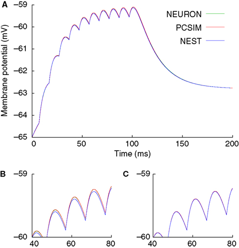
Figure 1. Results of running first example given in the text, with NEURON, NEST and PCSIM as back-end simulators. (A) Entire membrane potential trace with integration time-step 0.1 ms. (B) Zoom into a smaller region of the trace, showing small numerical differences between the results of the different simulators. (C) Results of a simulation with integration time-step 0.01 ms, showing greatly reduced numerical differences.
The low-level, procedural interface, using the
create(), connect() and record() functions, is useful for simple models or when porting an existing model written in a different language that uses the create/connect idiom. For larger, more complex networks we have found that an object-oriented approach, with a higher-level of abstraction, is more effective, since it both clarifies the conceptual structure of the model, by hiding implementation details, and allows behind-the-scenes optimizations.To illustrate the high-level, object-oriented interface we turn now from the simple example of a few neurons to a more complex example: a network of several thousand excitatory and inhibitory neurons that displays self-sustained activity (based on the “CUBA” model of Vogels and Abbott (2005)
, and reproducing the benchmark model used in Brette et al. (2007)
). This still is not a particularly complicated network, since it has only two cell types, no spatial structure and no heterogeneity of neuronal or connection properties, but in demonstrating how building such a network becomes trivial using PyNN we hope to convince the reader that building genuinely complex, structured and heterogeneous networks becomes manageable.
Again, we begin by choosing which simulator to use. We also import some classes from PyNN’s random module.
We next specify the parameters of the neuron model (the same model and same parameters are used for both excitatory and inhibitory neurons).
Parameters with dimensions of voltage are in millivolts, time in milliseconds and capacitance in nanofarads. The units convention is discussed further in the next section.
We now initialize the simulation, this time accepting the default values for the global parameters.

Now, rather than creating each cell separately, we just create a
Population object for each different type of cell:
By default, all cells of a given Population are created with identical parameters, but these can be changed afterwards. Here we wish to randomize the value of the membrane potential at the start of the simulation to values between −50 and −70 mV.
randomInit() is a convenience method for randomizing the initial membrane potential. For the more general case of randomizing any cell parameter use rset().Just as individual neurons are encapsulated within
Populations, connections between neurons are encapsulated within Projections. To create a Projection object, we need to specify how the neurons will be connected, either via an algorithm or via an explicit list. Different algorithms are encapsulated in different Connector classes, e.g.
FixedProbabilityConnector,AllToAllConnector. An explicit list of connections can be provided via a FromListConnector or a FromFileConnector.
Note that weights are in microsiemens and delays in milliseconds. Where the delay is not specified, the global minimum delay specified in the
setup() function is used. Here we set all weights and delays of a Projection to the same value, but it is equally possible to pass the constructor a RandomDistribution object, as we did above for the initial membrane potential, or an explicit list of values.To create a
Projection, we need to specify the pre- and post-synaptic Populations, a Connector object, and a synapse type. The standard IF cells each have two synapse types, “excitatory” and “inhibitory”. User-defined models can use arbitrary names, e.g. “AMPA”, “NMDA”.
Having constructed the network, we now need to instrument it, using the
record() (for recording spikes) and record_v() (membrane potential) methods of the Population objects. Here we choose to record spikes from 1000 of the excitatory neurons (chosen at random) and all of the inhibitory neurons, and to record the membrane potential of two specific excitatory neurons. We then run the simulation for 1000 ms.
After running the simulation, we can access the results or write them to file.
The results of running simulations of the above network with two different simulator back-ends are shown in Figure 2
.
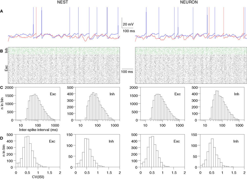
Figure 2. Results of running the second example given in the text, with NEURON and NEST as back-end simulators. Note that the network connectivity and initial conditions were identical in the two cases. (A) Membrane potential traces for two excitatory neurons. Note that the NEST and NEURON traces are very similar for the first 50 ms, but after that diverge rapidly due to the effects of network activity, which amplifies the small numerical integration differences. (B) Spiking activity of excitatory (black) and inhibitory (green) neurons. Each dot represents a spike and each row of dots a different neuron. All 5000 neurons are shown. (C) Distribution of pooled inter-spike intervals (ISIs) for excitatory and inhibitory neurons. (D) Distribution over neurons of the coefficient of variation of the ISI [CV(ISI)].
To achieve the goal of “write the code for a model once, run it on any supported simulator without modification” requires (i) a common interface, (ii) neuron and synapse models that are standardized across simulators, (iii) consistent handling of physical units, (iv) consistent handling of (pseudo-)random numbers. To achieve the twin goals of supporting a high-level of abstraction and facilitating porting of models between simulators requires both an object-oriented and a procedural interface. The implementation of all these requirements is described in more depth in the following. We also illustrate the mixing of PyNN and native simulator code, and how PyNN can support features that are found in only a single simulator back-end, by describing support for multi-compartmental models.
Standard Cell Models
A fundamental concept in PyNN is the cell type – a given model of a neuron, representable by a set of equations, and comprising sub-threshold behaviour, spiking mechanism and post-synaptic response. The public interface of a cell type is mainly defined by its parameters. Different neurons of the same cell type may have very different behaviour if they have different values of the parameters. For example, the Izhikevich model (Izhikevich, 2003
), can reproduce a wide range of spiking patterns, from fast-spiking through regular spiking to multiple types of bursting, depending on the parameter values chosen. A cell type is therefore a model type rather than a biologically defined cell type (such as “Layer V pyramidal neuron”, for example).
When using a given simulator back-end, PyNN can work with any cell type that is supported by that simulator. In this case, the cell type is generally represented by a string, holding a model name that is meaningful for that simulator, e.g. “
iaf_neuron” in NEST.Of course, such a cell type will only work with one simulator. To create a model that will run on different simulators requires you to use one of PyNN’s built-in, standard cell models, each represented by a sub-class of the
StandardCell class. The models provided by PyNN include various simple IF models, the Izhikevich-like adaptive exponential IF model (Brette and Gerstner, 2005
), a single-compartment neuron with Hodgkin–Huxley sodium and potassium channels, and various models that emit spikes (e.g. according to a Poisson process) but cannot receive them.The
StandardCell class contains machinery for translating model names, parameter names and parameter units between PyNN standardized values and simulator-specific values. This is particularly useful when the underlying simulators use different unit systems or different parameterizations of the same set of equations, e.g. when one simulator expects the membrane time constant and another the membrane leak conductance. An example of the translations performed by PyNN is given in Table 1
.
Currently, all the standard cell types are single-compartment or point neuron models, since PyNN currently supports only one simulator for multi-compartmental models (NEURON). Further details on using multi-compartmental models with PyNN’s NEURON back-end are given below. We plan in future to allow specifying multi-compartmental cell types using a NeuroML description (Crook et al., 2005
).
Units
As is clear from the previous section, each simulator back-end has its own convention for which units to use for which physical quantities. The exception to this is Brian, which has a system for explicitly specifying units and for checking that equations are dimensionally consistent. In the future, we plan to adopt Brian’s system for PyNN, but for now we have chosen to use a convention, which is similar to that of NEURON and NEST in that the units are those that tend to be used by experimental physiologists. An alternative would have been the convention used by PCSIM (and also by the GENESIS simulator) of using pure SI units with no prefixes. The advantage of the latter convention is that there is no need for checking equations for dimensional consistency. The disadvantage is that numerical values in such a system are often very large or very small, and hence the human intuition for reasonable and unreasonable parameter values is mostly lost.
Irrespective of the relative merits of different conventions, the most important thing is that PyNN now provides a single convention which is valid across simulators. In detail, the convention is as follows: voltage – mV, current – nA, conductance – μS, time – ms, capacitance – nF.
Standard Synapse Models
In PyNN, the shape and time-course of the elementary post-synaptic current or conductance change in response to a pre-synaptic spike are considered to be a part of the post-synaptic neuron model, while all other properties of a synaptic connection, notably its weight (the peak current or conductance of the synaptic response), delay (for point models, this implicitly includes axonal propagation, chemical transmission and dendritic propagation; more morphologically and/or biophysically detailed models may model explicitly some or all of these sources of delay), and short- and long-term plasticity, are considered to depend on both pre- and post-synaptic neurons, and so are encapsulated in the concept of “synapse type” that mirrors the “cell type” discussed above.
The default type of synaptic connection in PyNN is static, with fixed synaptic weights. To model dynamic synapses, for which the synaptic weight (and possibly other properties, such as rise-time) varies depending on the recent history of post- and/or pre-synaptic activity, we use the same idea as for neurons, of standardized, named models that have the same interface and behaviour across simulators, even if the underlying implementation may be very different.
Where the approach for dynamic synapses differs from that for neurons is that we attempt a greater degree of compositionality, i.e. we decompose models into a number of components, for example for short-term and long-term dynamics, or for the timing-dependence and the weight-dependence of STDP rules, that can then be composed in different ways.
The advantage of this is that if we have n different models for component A and m models for component B, then we require only n + m models rather than n × m, which had advantages in terms of code-simplicity and in shorter model names. The disadvantage is that not all combinations may exist, if the underlying simulator implements composite models rather than using components itself: in this situation, PyNN checks whether a given composite model AB exists for a given simulator and raises an Exception if it does not. The composite approach may be extended to neuron models in future versions of the PyNN interface depending on the experience with composite synapse models.
Currently only a single model exists in PyNN for the short-term plasticity component, the Tsodyks–Markram model (Markram et al., 1998
). For long-term plasticity there is a spike-timing-dependent plasticity STDP component, which itself is composed of separate timing-dependence and weight-dependence components.
Low-Level, Procedural Interface
We refer to the procedural interface as “low-level” because it deals with a lower level of abstraction – individual neurons and individual synapses – than the object-oriented interface. The procedural interface consists of the functions
create(), connect(), set(), record() (for recording spikes) and record_v() (for recording membrane potential). Each of these functions operates on, or returns, either individual cell ID objects or lists of such objects. As was described in the Usage Examples section, as well as being passed around as arguments, the ID object may be used for accessing/
modifying the parameters of individual neurons, and takes care of parameter translation using the StandardCell mechanisms described above.It is possible to some extent to mix the low-level and high-level interfaces. For example, it is possible to access individual neurons within a
Population as ID objects and then use the connect() function to connect them, instead of using a Projection object.Why have both a low-level and high-level interface? Having both is a potential source of confusion for users and is definitely a maintenance burden for developers. The main reason is to support the use of PyNN as a porting tool. The majority of neuronal network models using existing simulators use a procedural approach, and so conversion to PyNN is easier if PyNN supports the same approach. In addition, when developing a PyNN interface for a simulator, or for neuromorphic hardware, that deals primarily with individual cells and synaptic connections, it is easier to implement only the low-level interface, since the high-level interface can be built upon it.
High-Level, Object-Oriented Interface
Object-oriented programming has been used for many years in computer science as a method for reducing program complexity. As the ambition and scope of large-scale, biologically detailed neuronal network modelling increases, reducing program complexity will become more and more critical, as the limiting factor in computational neuroscience becomes the productivity of the programmer and not the capacity of the computer (Wilson, 2006
). It is for this reason that the preferred interface in PyNN for developing new models is an object-oriented one.
The object-oriented interface is built around three main classes:
Population – a group of cells all with the same cell type (model type). It is generally considered that the cells in a
Population should all represent the same biological cell type, i.e. although parameter values may vary between cells in the group, all cells should have qualitatively the same firing response. This is not enforced, but is a good guideline to follow for producing understandable code. The Population class eliminates tedious iteration over lists of neurons and enables more efficient, array-based management of neuron properties.Projection – the set of connections of a given synapse type between two
Populations. Creating a Projection requires specifying the pre- and post-synaptic Populations, the synapse type, and the algorithm used to determine which neurons connect to which.Connector – an encapsulation of the connection algorithm used in creating a Projection. Simple examples of such algorithms are “all-to-all”, “one-to-one” and “connect-each-pre-and-post-synaptic-cell-with-a-fixed-probability”. It is also possible to provide an explicit list of which cells are to be connected to which others. Each algorithm is defined within a subclass of the
Connector class. PyNN contains a number of such classes, but it is fairly straightforward for a user to define their own algorithms.In future development of PyNN, we plan to extend the interface to still higher-level abstractions, such as layers, cortical columns, brain areas and inter-areal projections. We also aim to use the high-level interface as a link between spiking network models and more abstract models that do not represent individual neurons, such as mean-field models.
Random Numbers
The central nervous system contains many sources of noise, and activity patterns are often sufficiently complex, and possibly chaotic, to make a stochastic representation a reasonable model.
This can become a problem when comparing the behaviour of a given model run on different simulators, since random differences might obscure real inconsistencies between implementations of the model. Similarly, when performing distributed computations on parallel machines, the model behaviour should not depend on the number of processors used (Morrison et al., 2005
), and random differences can conceal real differences between the parallel and serial implementations.
For these reasons, it is important to be able to use identical sequences of random numbers in different simulators, and to have the random number used at a particular point in the program execution be independent of which processor it is running on.
Another consideration is that simulations in most cases use only pseudo-random sequences, and low-quality random number generators (RNGs) may have correlations between different elements of the sequence that can significantly affect the qualitative behaviour of a network. Hence it is necessary to be able to test the simulation with different RNGs.
PyNN supports simulator-independent RNGs and use of different generators – currently any of the generators provided by the
numpy package or by the GNU Scientific Library (GSL) can be used.This is done by wrapping the
numpy and GSL RNGs in classes with a common interface. PyNN’s random module contains the classes NumpyRNG and GSLRNG, which both have a single method, next(n, distribution, parameters), which returns n random numbers from a distribution of type distribution with parameters parameters, e.g.
Since all PyNN code that uses random numbers accesses the RNG classes only through this
next() method, a user can substitute their own RNG simply by defining a wrapper class with such a method.Since very often one wishes to use the same random distribution repeatedly, rather than changing distribution each time, the
random module also provides the RandomDistribution class, which is initialized with the distribution name and parameters, and thereafter the next() method is simplified to take a single argument, the number of values to draw from the distribution, e.g.
Note that NumpyRNG and GSLRNG distributions may not have the same names, e.g. “normal” for
NumpyRNG and “gaussian” for GSLRNG, and the arguments may also differ. One of our future plans is to extend the random module in order to harmonize names across RNGs.Multi-Compartmental Models
PyNN currently supports only a single simulator, NEURON, that is suitable for many-compartment models. Given the principle of supporting simulator-independence only for features that are shared by at least two of the supported simulators, and given PyNN’s focus on network modelling, PyNN does not provide an API for specifying simulator-independent multi-compartmental models. This is a possible future development – preliminary work has been done on a PyNN interface to the MOOSE simulator (Ray and Bhalla, 2008
) – but a more likely path would be to make use of the NeuroML standards for specifying multi-compartmental models. In this scenario, the filename of a NeuroML level 2 file, specifying a single cell type, would be passed as the
cellclass argument to the PyNN create() function or Population constructor.However, since native and PyNN code can be mixed, the
pyNN.neuron module already supports simulations with multi-compartmental models. The pre-synaptic compartment whose voltage is watched to trigger synaptic transmission (e.g. axon terminal) can be specified using the source argument to the Projection constructor, and the post-synaptic mechanism specified with the target argument.Debugging
Should an error occur in a PyNN simulation, a good first step is to re-run it on another simulator back-end and so narrow down the source of the problem to one back-end in particular. Nevertheless, it has proven to be the case that the additional layers of abstraction provided by PyNN sometimes make it harder to track down sources of errors. To counterbalance this, PyNN traps errors coming from the simulator core and employs Python’s introspection capabilities to provide additional information about the error context. For example, if an invalid parameter name is provided to a neuron model, the error message lists all the valid parameter names for that model. Furthermore, logging can be switched on via the
init_logging() function in the pyNN.utility module, causing detailed information about what the system is doing to be written to file, a valuable resource for tracking down bugs.PyNN is both a definition of a common simulator interface and an implementation of this interface for each supported simulator. PyNN is implemented as a Python package containing a
common module, which defines the API and contains functionality common to all simulator back-ends, a random module (described above), and a module for each simulator back-end, as shown in Figure 3
. Each simulator module separately implements the API, although it can make use of much shared code in common. In most cases, the simulator modules have been implemented by, or in close collaboration with, the simulator developers.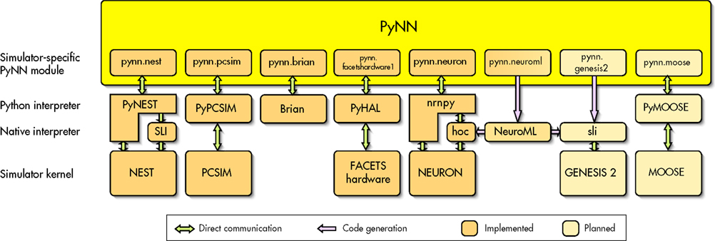
Figure 3. The architecture of PyNN.
PyNN currently fully supports the following simulators: NEURON (Carnevale and Hines, 2006
; Hines and Carnevale, 1997
; Hines et al., 2008
), NEST (Eppler et al., 2008
; Gewaltig and Diesmann, 2007
), PCSIM (http://www.lsm.tugraz.at/pcsim/
) and Brian (Goodman and Brette, 2008
). Support for MOOSE (Ray and Bhalla, 2008
) and for export in NeuroML format (Crook et al., 2005
) is under development.
PyNN also supports the Heidelberg neuromorphic hardware system (Schemmel et al., 2007
). This illustrates a major benefit of the existence of a common neuronal simulation interface: novel simulation or emulation systems do not need to develop their own programming interface, but can benefit from an existing one that guarantees interoperability with existing tools. Using PyNN as the interface to neuromorphic hardware systems provides the possibility of closing the gap between the two domains of numerical simulation and physical emulation, which have so far coexisted rather separately.
For a given model with a given parameter set run on a given version of a given simulator, it should be possible to exactly reproduce a simulation result, independent of computer architecture (except where this affects the precision of the floating-point representation) or operating system. For parallel systems, results should also be independent of how many threads or processes are used in the computation, although here exact quantitative reproduction is harder to achieve. Reproducibility across different versions of a given simulator is not essential provided the precise version used to generate a given result is specified, but it is of course highly desirable. When running a model on different simulators, exact reproduction is impossible to achieve, except in simple cases, due to round-off errors in floating point calculations. When validating a model implementation by running it on two or more simulators, therefore, what level of reproducibility is achievable, and how can we tell whether any differences are due to round-off error or to implementation errors?
To get a preliminary handle on this problem, we have compared the difference in model activity between two simulators to the difference due to two different initial conditions with the same simulator.
Our test case is the balanced random network, based on Vogels and Abbott (2005)
, whose implementation was shown above. The activity pattern of this network is very sensitive to initial conditions (chaotic or near-chaotic), and so we cannot use differences in the precise spike pattern to measure reproducibility: we are more interested in the statistical properties of the activity, and so we have chosen to take the distribution of inter-spike intervals (ISIs) of excitatory neurons (see Figure 2
C) as a measure of network activity.
To measure the difference between the distributions from two different runs we use the Kolmogorov–Smirnov two-sample test. We ran the simulation ten times, each time with a different seed for the RNG used to generate the initial membrane potential distribution, with both NEURON and NEST back-ends. This gave values for the Kolmogorov–Smirnov D-statistic between 0.008 and 0.026 (n  19000) with a mean of 0.015, with associated p-values (probability that the two distributions are the same) between 6.3 × 10⁻⁵ and 0.68 with mean 0.15.
19000) with a mean of 0.015, with associated p-values (probability that the two distributions are the same) between 6.3 × 10⁻⁵ and 0.68 with mean 0.15.We then ran the simulation twenty times just on NEURON, each time with a different RNG seed, to give 10 pairs of distributions. In this case the D-values were in the range 0.007–0.026, mean 0.015, and the p-values in the range 2.8 × 10⁻⁵ to 0.77, mean 0.20.
In summary, the differences due to different simulators are in almost exactly the same range as those due to different initial conditions, suggesting that the differences between the simulators are indeed due to round-off errors and that there are not, therefore, any implementation errors in this case.
It is also interesting to note that in most cases the null hypothesis is supported, i.e. the distributions are the same, but that for some initial conditions there are highly significant differences between the ISI distributions. The ISI distribution may not therefore be the best measure for reproducibility in this case.
In this article we have presented PyNN, a Python-based common simulator interface, which allows simulator-independent model specification. PyNN is already in use in a number of research groups, and has been a key technology enabling improved communication between labs in a pan-European collaborative project with a major component of modelling and of neuromorphic hardware development (the FACETS project: http://www.facets-project.org
).
By providing a standard simulation platform, PyNN also has the potential to act as the foundation for other, simulator agnostic but neuroscience-specific, tools such as analysis, visualization and data-management software.
PyNN is not the only project to address simulator-independent model specification and simulator interoperability (review in Cannon et al., 2007
). neuroConstruct (Gleeson et al., 2007
) is a tool to develop networks of morphologically-detailed neurons using a graphical user interface (GUI), that can generate code for both the NEURON and GENESIS simulators. A limitation with respect to PyNN is that since it uses code generation rather than a direct interface, neuroConstruct cannot receive information back from the simulator except by reading the data files it generates. A second limitation is that features that are not available through the GUI cannot be incorporated in a model. The NeuroML standards (Crook et al., 2005
, http://www.neuroml.org
) are intended to provide an infrastructure for exchanging model specifications between groups in a simulator-independent way. Their scope includes much more detailed levels of modelling, e.g. membrane ion channels and detailed dendritic morphology, than are supported by PyNN. They have the advantage over PyNN of being language-independent, since specifications are written in XML, for which tools exist in all major programming languages. The major disadvantage of purely declarative specifications is lack of flexibility: if a concept or entity is not defined in the standard, it is not possible to specify models that use it, whereas with a procedural/imperative or mixed declarative-procedural specification such as is achievable with PyNN, arbitrary specifications are possible.
Although we emphasize here the differences between the GUI, pure-declarative, and programming-interface approaches to simulator-independent model specification, in fact they are highly complementary. Graphical interfaces are particularly good for beginners, for teaching, for giving high-level overviews of a system, and for integrating analysis and visualization tools. It would be very useful for neuroConstruct to be able to generate PyNN code, for example, in addition to code for NEURON and GENESIS. Declarative specifications reach the highest levels of system-independence, for the range of concepts that are supported. They are also particularly suitable for transformation into human-readable formats and for automated GUI generation. As such, they seem to be best suited for domains in which the modelling approach is fairly stable, e.g. for describing neuron morphologies or non-stochastic ion channel models. In PyNN, we plan to support simulator-independent multi-compartmental models using NeuroML: in this scenario cell models would be specified in NeuroML while PyNN would be used for network specification and for simulation setup and control.
Our main priorities for future development of PyNN are to increase the number of supported simulators (simulator developers who are interested in PyNN support for their simulator are encouraged to contact us), improve the support for multi-compartmental modelling, and extend the interface towards higher-level abstractions, such as cortical columns and more abstract modelling approaches. PyNN is open source software (CeCILL licence, http://www.cecill.info
) and has an open development model: anyone who wishes to contribute is welcome and invited to do so.
The authors declare that the research was conducted in the absence of any commercial or financial relationships that could be construed as a potential conflict of interest.
This work was supported by the European Union (FACETS project, FP6-2004-IST-FETPI-015879). Jens Kremkow is also supported by the German Federal Ministry of Education and Research (BMBF grant 01GQ0420 to BCCN, Freiburg).
Brette, R., Rudolph, M., Carnevale, T., Hines, M., Beeman, D., Bower, J., Diesmann, M., Morrison, A., Goodman P. H., Harris, F. Jr, Zirpe, M., Natschlager, T., Pecevski, D., Ermentrout, B., Djurfeldt, M., Lansner, A., Rochel, O., Vieville, T., Muller, E., Davison, A., El Boustani, S., and Destexhe, A. (2007). Simulation of networks of spiking neurons: a review of tools and strategies. J Comput. Neurosci. 23, 349–398.
Ekeberg, Ö., and Djurfeldt, M. (2008). MUSIC – multisimulation coordinator: request for comments. Nat. Precedings http://dx.doi.org/10.1038/npre.2008.1830.1
.
Schemmel, J., Brüderle, D., Meier, K., and Ostendorf, B. (2007). Modeling synaptic plasticity within networks of highly accelerated I&F neurons. In Proceedings of the 2007 IEEE International Symposium on Circuits and Systems (ISCAS’07). New Orleans, IEEE Press, pp. 3367–3370. doi: 10.1109/ISCAS.2007.378289.