Machine Learning in Football Betting: Prediction of Match Results Based on Player Characteristics


1
Department of Statistics and Econometrics, University of Erlangen-Nürnberg, Lange Gasse 20, 90403 Nürnberg, Germany
2
Department of Marketing Intelligence, University of Erlangen-Nürnberg, Lange Gasse 20, 90403 Nürnberg, Germany
3
FOM Hochschule für Oekonomie & Management, Zeltnerstraße 19, 90443 Nürnberg, Germany
*
Author to whom correspondence should be addressed.
Appl. Sci. 2020, 10(1), 46; https://doi.org/10.3390/app10010046
Submission received: 1 November 2019
/
Revised: 7 December 2019
/
Accepted: 13 December 2019
/
Published: 19 December 2019
Abstract
:In recent times, football (soccer) has aroused an increasing amount of attention across continents and entered unexpected dimensions. In this course, the number of bookmakers, who offer the opportunity to bet on the outcome of football games, expanded enormously, which was further strengthened by the development of the world wide web. In this context, one could generate positive returns over time by betting based on a strategy which successfully identifies overvalued betting odds. Due to the large number of matches around the globe, football matches in particular have great potential for such a betting strategy. This paper utilizes machine learning to forecast the outcome of football games based on match and player attributes. A simulation study which includes all matches of the five greatest European football leagues and the corresponding second leagues between 2006 and 2018 revealed that an ensemble strategy achieves statistically and economically significant returns of 1.58% per match. Furthermore, the combination of different machine learning algorithms could neither be outperformed by the individual machine learning approaches nor by a linear regression model or naive betting strategies, such as always betting on the victory of the home team.
1. Introduction
In recent decades, football has continued to draw worldwide attention from people of various ages and social situations. The game result is, like in most other sports, is usually used to assess the performance and success of a team or a single player. Given the importance of the score, it is hardly surprising that many gamblers try to guess the result of football matches. The motivation is on the one hand driven by the admiration of other enthusiasts, on the other hand monetary rewards serve as an incentive system.
This manuscript introduces a methodology for estimating the results of football matches using techniques from the field of machine learning. The corresponding data base consists of a large number of features which incorporate game characteristics as well as proportions of all soccer players from both teams. For this purpose, a comparison of different approaches was conducted to assess whether more complex algorithms are capable of better predicting football betting. To this end, the forecasts were verified by the betting odds of the market leader in online gambling. The out-of-sample results of our statistical arbitrage showed continuously positive returns over the entire period.
The most important enhancements to literature are the following. First of all, we designed a trading framework for betting on football matches based on machine learning approaches and methods of statistical arbitrage trading. Second, we conducted a simulation study based on a data set including in total 40 features for each player for 47,856 football matches of the big five football leagues and the corresponding second leagues from 2006 to 2018. Third, we challenged our strategies based on machine learning with traditional approaches in this area. The results of advanced quantitative methods are far superior compared to the benchmark strategies. Finally, we merged various machine learning algorithms into one ensemble-approach which showed more robust properties than any of the uncombined machine learning approaches.
The rest of the article is organized as follows. Section 2 gives a summary of the associated work. After discussing the dataset and the backtesting study in Section 3, we conduct a performance analysis in Section 4. Lastly, Section 5, concludes the manuscript and provides an outlook on future work. In this article, the term “football” is associated with the world’s most popular sport football (soccer).
2. Related Work
2.1. Literature on Sports Betting
2.1.1. Financial Markets and Betting
Some literature focuses on the efficiency of betting exchange markets. Reference [1], for example, noted during an analysis of the betting exchange market during the 2002 FIFA World Cup that there is only limited support for the hypothesis of efficient betting markets. Reference [2], on the contrary, published result of a similar study and revealed a fast and full adjustment of prices. They found that after a goal an immediate increase of the prices and noted that these prices remained higher even 10 to 15 min after. Reference [3] examined the market for the Spanish football leagues. They discovered out that the relative number of fans of each club in a match has an influence on betting odds in a way that supporters of more a popular team were offered better betting odds. Reference [4] compared the forecasting accuracy of bookmakers to a frequently used betting exchange and [5] analyzed the inter-market arbitrage in sports betting. They found out that combining data from bookmakers and information from the bet exchange market can lead to guaranteed positive returns. In addition, empirical studies and meta-studies regarding the prediction accuracy of experts and the bet exchange market predicting the outcome of a sporting event were published [6,7]. Reference [8] examined the behavior after unanticipated events using data form the in-play football betting market. They discovered that most participants under-react to anticipated events while over-reacting to events that were very surprising.
Furthermore, some publications analyzed the influence of match results of publicly traded sports teams on their stock prices. Reference [9] examined how football team stocks responded to the outcome of a match. They discovered that abnormal returns for winning teams are not reflected by rational expectations, but rather by overreactions induced by the investor’s sentiment. Reference [10] analyzed the difference between sports betting markets and financial markets for NFL football teams and revealed that, due to the capability of bookmakers to adjust their prices, they generate more profit than they could make by behaving like traditional brokers who attempt to balance supply and demand. Reference [11] investigated whether investors’ biased ex-ante beliefs towards the outcomes of a future event could be explained by inefficient stock markets. They assessed data about stocks of publicly traded European football clubs during important matches and discovered that investors’ sentiments are attributable to some extend for a systematic bias in their ex-ante expectations.
2.1.2. Forecasting the Outcomes of Sporting Events
Other articles about the prediction of the outcome of football games refer to major sporting events, such as the FIFA World Cup or the UEFA Euro Cup. Reference [12] introduced a least squares betting approach in 1980 and applied it to data about the FIFA World Cup 1976. Reference [13] described a betting strategy based on the Fibonacci sequence. During a simulation on FIFA World Cup finals, they found that one could make economic profits through employing this method with a fairly large risk. Reference [14] published an empirical study comparing the prediction accuracy for the FIFA World Cup 2006 to predictions derived from the FIFA world ranking. They discovered that prediction markets for the FIFA World Cup outperform forecasts based on the FIFA world ranking in terms of accuracy. Reference [15] proposed a probabilistic prediction method for the 2018 FIFA World Cup based on the bookmaker consensus model to identify the winner of the FIFA World Cup. Two years before, they also predicted the winner of the UEFA Euro Cup [16] based on a similar strategy.
In addition to the prediction the FIFA World Cup, Reference [12] forecast with a least squares betting approach the results of other sporting events in American football and basketball. Moreover, Reference [17] examined a betting strategy analyzing about 500 tennis matches and revealed a cumulative return of 16%.
2.1.3. Forecasting Football League Match Results
Since this article aims to forcast the results of football league matches based on characteristics and skills of the involved football players, we could identify a few publications related to this topic:
- Reference [18] extracted time dependent skills of teams of the English Premier League as well as the Spanish Primera Division with a Bayesian dynamic generalized linear model. They employed an algorithm to find the parameters of their model and to predict the next football matches based on results of former matches. In total they examined 3892 football matches from 1993 to 1997 and yielded a final cumulative return of 40% (English Premier League) and 54% (Spanish Primera Division).
- Reference [19] predicted Premier League football games by incorporating Twitter Microposts in which users estiamated the outcome of a football match. Thus, these data were yielded from textual information by a parsing algorithm. For 200 matches in 2013/2014, they could realize a profit of about 30%.
- Reference [20] made predictions for match outcomes of the Dutch Eredivisie from 2000 to 2013. The data set uased included of the results of the former matches. Moreover, they added data about whether teams played in a lower leagues in the football season before, about whether a new coach was hired, and whether a top scorer of a team was injured. Different machine learning algorithms were analyzed based on these data regarding their prediction ability (e.g., Decision trees, Neural Networks, and Naive Bayes).
- References [21,22] predicted the football matche results extracting the characteristics of the corresponding teams. They exploited this information incorporating a risk-averse betting strategy. Based on in total 8082 football matches from 2013 to 2018, the authors could achieve economically as well as statistically significant returns.
In conclusion, none of these publications analysed the topic this paper focuses on. Some articles aim to connect sports betting with different financial markets [1,5,8] while others predict specific sporting events [12,15,17]. Currently, there is neither a study about incorporating player characteristics (e.g., age, weight, weight) and player skills (e.g., ball control, dribbling, crossing) nor one which predicts football matches for the big five football leagues (England, France, Germany, Italy, Spain) and the corresponding second leagues. This article fills these and other gaps.
2.2. Publications about Statistical Arbitrage
Statistical arbitrage was developed in the mid-eighties by a group of mathematicians and physicists at Morgan Stanley with the aim to use the approach as a trading strategy. Statistical arbitrage is a long-term trading opportunity which exploits capital market anomalies to generate profits over time. Based on a variety of methods, including models from computer science, operations research, physics, and mathematics, trading recommendations are extracted.
In recent years, there was a noticeable increase of interest in the academic community regarding statistical arbitrage trading. Publications in this field analyzes theoretical principles and empirical applications, e.g., [23,24,25,26,27,28]. So far, only two studies presenting a statistical arbitrage strategy in the field of sports betting exist [22,29]. In stark contrast to these articles, our study analyzes a much higher amount of matches based on many more variables, such as characteristics and skills of each football player involved.
3. Simulation Study
3.1. Data Sources
Our algorithms amassed data from football matches of the Premier League, Football League Championship (England), Ligue 1, Ligue 2 (France), Bundesliga, Bundesliga 2 (Germany), Serie A, Serie B (Italy), Primera Division, Segunda Division (Spain) from season 2006/2007 to 2017/2018. This record of 47,856 football matches provides a true hardness test for any backtesting study, as investor interest and analyst scrutiny are particularly high for these football nations. To date, 25 of the 27 Champions League winners come from these countries. This supremacy is further demonstrated by the coefficient ranking, which reflects the results achieved in the past: Of the top 20 teams, 17 are from the considered countries. In the rare event that a match result was later modified by a judge for other causes, we continued on using the original result instead. Detailed explanations of the data set follow in the next sections.
3.1.1. Player Characteristics and Skills
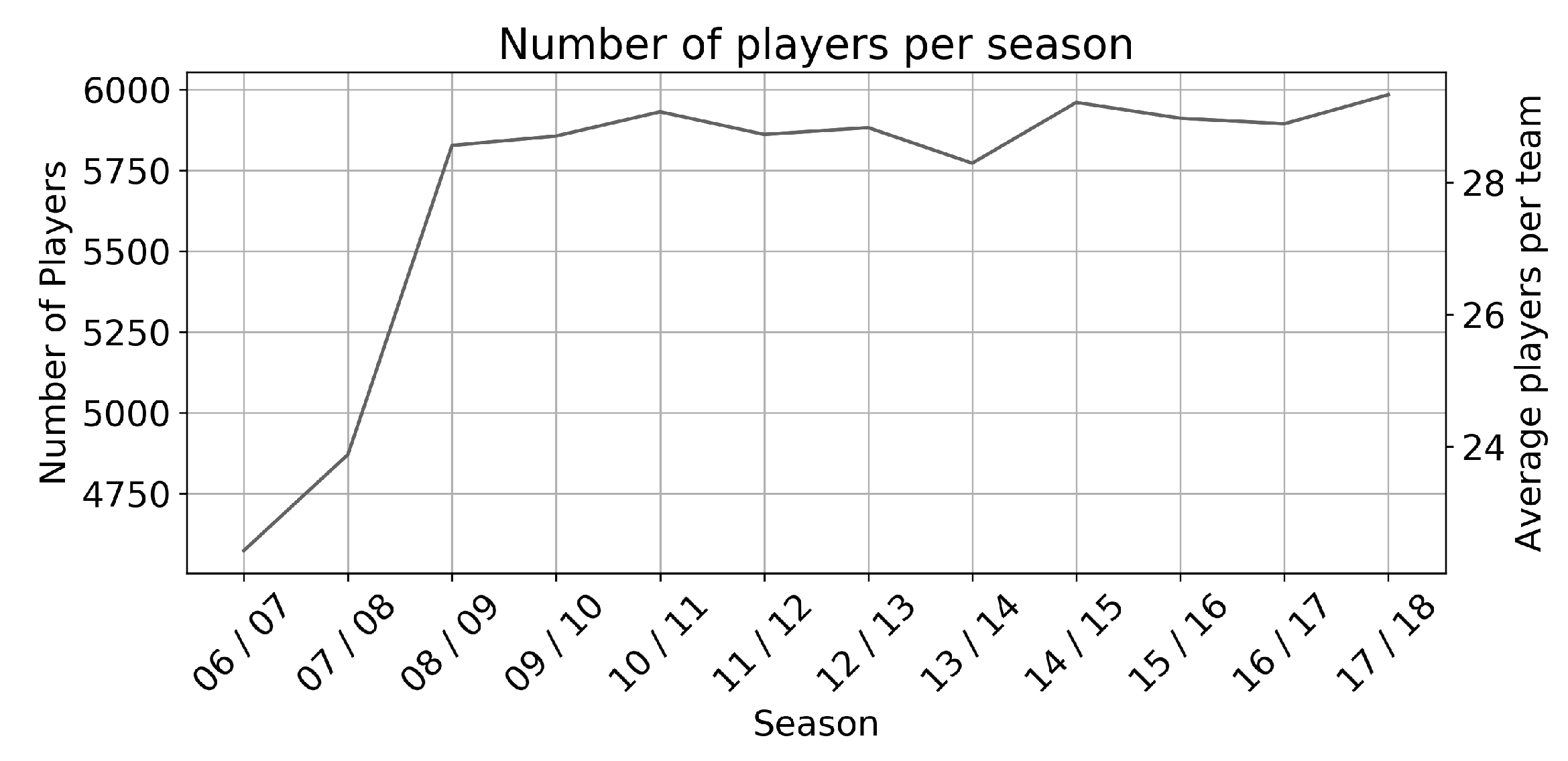
Baseline for our simulation study are several characteristics and skills on player level, reported and collected prior of each season (We are grateful to https://www.fifaindex.com for supplying the information.). Figure 1 gives an overview on the size of data that has been available for each season. Overall, we used statistics of 19,998 different players, with a total of 204 teams across the 10 leagues for each season. In total, we have 68,323 observations, as many players are reported across several seasons. Interestingly, there is a sharp increase in players information available each season from 2006/2007 to 2008/2009—after that season, the number of players remains on the same level (around 6000 players per season).
Table 1 shows descriptive statistics of individual features and skills of all football players used for our machine learning approach. To be more specific, we consider the body measures, pass accuracies, agility, reaction, and aggression for every player that has been part of a the five European major leagues (first and second league each). Most of those variables are within a range from 1 to 100—however, the maximum value of 100 has never been associated with any player so far.
3.1.2. Match Results
This manuscript aims to predict the results of football matches based on different machine learning approaches. Therefore, Figure 2 presents the goal difference of two teams in more detail.
Altogether 21,698 home victories (45.3%), 12,895 draws (27%) and 13,253 away victories (27.7%) were achieved. These results clearly demonstrate the home advantage, which is also reflected in the match attributes. This is consistent with the observation that the distribution of goal difference (home goal minus away goal) is not symmetric. We observe fewer matches with a negative goal difference (away victories) than with a positive goal difference (home victories). Nevertheless, the main event was a draw, i.e., the number of goals scored by the home team is equal to the number of goals scored by the away team.
3.1.3. Betting Odds
In addition to player characteristics and scores, this research paper also uses the corresponding odds from online bookmaker Bet365, which is one of the leading betting providers with around 23 million customers (We are grateful to https://www.football-data.co.uk/data.php for supplying the information.). By including this data, we can evaluate the performance in the financial context as well as a statistical evaluation. For this purpose, our trading strategy uses the usual decimal ratios: We put a bet amount b on a certain event, which is provided with a certain odds o. Once the event happens, the bet amount is multiplied by the bet of odd . Nothing will be paid if the event does not take place. Thus, the relative profit on b is either (for a successful bet) or , i.e., a complete loss of b, for an unsuccessful bet.
Figure 3 explains the counterplay between the probabilities for the three outcomes and the resulting bets. The betting odd is the inverse of the respective probability of an outcome. Especially in the context of sports betting, this representation is more intuitive as it links directly to the potential payout amount rather than the probabilities. However, bookmakers usually diminish the fair odd value by a certain amount to cover their costs in the long run.
A summary of the accumulated odds is given in Table 2. Remarkably, we observe more extreme odds for one of the team than for a draw. Not surprisingly, the bookmaker is familiar with the well-known home advantage—the average odds of a home win (2.42) are significantly below the average odds for an away win (4.27).
3.2. Simulation Design
The objective of the simulation study was (1) to predict football matches with the help of data-driven methods and (2) to exploit the obtained information in order to constrcut a statistical arbitrage strategy. In particular, we predicted goal difference between the home and away teams (dependent variable y) based on different machine learning approaches. Our models are trained on player characteristics and skills, observed before the start of each season (independent variables x). We divided each season into a formation period and a trading period. In order to avoid the look-ahead-bias, we split the two sets by a specific date.
3.2.1. Formation Period
The formation period includes the results and characteristics of the first five match days of each season. However, since our players characteristics are only reported prior to each season, we keep them constant as we are iterating through the match days. Thus, we implicitly assume them to be constant over season. To capture short term highs and lows, we also consider a teams performance using a lagged time window of 5 match days (if possible). Since the formation period contains the first five match days, we have 490 matches for training our model. Each additional matchday is the test phase, which is why we predict 90 games there.
specifies the difference in goals between the home team and the away team and is created using the players characteristics and the corresponding team performance measure. The features of include the characteristics from the areas “General”, “Ball Skills”, “Passing”, “Shooting”, “Defense”, “Physical”, “Mental”, and “ Goalkeeper”(see Table 1). Of course, we do not consider all players of a team but only the players who are on the field. As starting line-up we use the players declared by FIFA. Therefore, injured or blocked players will not be considered—this procedure is very similar to reality. For all features (except the goalkeeper features) we sort each players values (that is not a goalkeeper) of each team and average the top 4 values. The number 4 is derived from the fact that in one position, one does rarely find more than 4 players at the time. Features concerning the goalkeeper only use player data from goalkeepers.
We describe the relation of the dependent variable as a function of the 41 independent variable . Therefore, the underlying function is created by the following machine learning approaches:
- Random forest (RAF): Random forest (In this context we use regression trees rather than classification trees.)combines several uncorrelated decision trees to output a weighted prediction of each tree. Most important, it can handle both, numeric and categorical input which makes it a good choice for a initial model. Overfitting to the formation period is avoided by correcting the habit of decision trees. For further details about this approach, see [30,31].
- Support vector machine (SVM): Support vector machine splits objects into categories, ensuring that no objects are located in the area around the estimated boundaries. As in most cases, we used the kernel trick in order to handle the case of non-linear separable data. References [34,35] explained the concept of SVM.
- Linear regression (LIR): Finally, we benchmarked the approsches with a classic linear regression. Consequently, statistical properties of this naive model can easily be shown. For further details about this approach, see [36].
The choice of the four machine learning methods is motivated by [37]. The authors give an excellent overview of the advantages and disadvantages of different learning algorithms based on existing empirical and theoretical studies. As a strong regression model we introduce the equally weighted ensemble ALL, which integrates the information of the approaches RAF, BOO, SVM and LIR. To be more precise, we calculate the average prediction of these four baseline approaches. According to [38,39], the use of ensembles in machine learning has two major advantages: First, we have a statistical advantage by reducing the risk of selecting the wrong regression model. Second, allowing combinations of several hypotheses significantly increases the solution space of our dependent variable. In summary, our equally weighted ensemble ALL is an efficient and robust approach.
3.2.2. Trading Period
After the formation period, the models have been applied consecutively to each match day, beginning with match day 6. This results in the predictions which we denote as . We received the dependent variable by applying the learned models (RAF, BOO, SVM, LIR) as well as the player features . The trading period contains data from the sixth match day until the final match day of each season. This simulation study assumed that players characteristics include important knowledge influencing future football matches. If our assumptions holds, the trading algorithm would be able to find market anomalies and to generate positive profits. We define the following trading signals:
- If , we forecast that the home team wins. In consequence, we invest 1 monetary unit () on the bet “home team wins”.
- If , we forecast that the away team wins. In consequence, we invest 1 monetary unit () on the bet “away team wins”.
- If , we forecast no clear victory of home team or away team. In consequence, no trading is conducted.
We calculate the profits of each bet based on the available odds. If we bet on the home team (away team) and actually observe a win of the home team (away team), then the payout of the bet equals the corresponding betting odd. In another case, the payout is 0, i.e., we lose our monetary unit. We use the difference in goals as a kind of confidence measure. We argue that predicting a draw is way harder due to incorrect decisions and penalties than a clean win. Following the large-scale research studies of [40,41], the trading thresholds of are implemented. Following [42,43], our trading strategy is based on the finding that trading strategies with the use of machine learning can significantly improve the overall performance.
In the spirit of [44], we benchmark the strategies based on one single machine learning algorithm each against four strategies. The strategy ALL trades, if the average of the predicted goal differences yields less than −2 or more than +2. Having an average this extreme can result from two scenarios: either many of the algorithms come to similar, extreme predictions or one algorithm is extremely confident. In both cases, we have strong indication to place a bet on the predicted outcome. If the four machine learning predictions are quite different to each other, their average would be close to zero. In a way, the uncertainty from distinct predictions makes the ALL strategy not place a bet (conservative strategy).
Furthermore, three baseline strategies served as a benchmark, one of which is derived directly from the betting odds: (1) Strategy BET bets on the event with the lowest odd (most probable outcome). As explained in the previous section, the lowest betting odd is always achieved by “home team wins” or “away team wins”. (2) Strategy HOM bets 1 monetary unit on “home team wins” which reflects the well-known advantage of a team playing in their home stadium, see e.g., Table 2. Other information are not considered. (3) Strategy RAN randomly bets on the event “home team wins” or “away team wins”.
4. Results
4.1. Statistical Analysis
We provide an overview of some basic statistics of the simulation study in Table 3. The columns summarize the different betting strategies and/or methods described in the previous section—row-wise we list the measures of performance. Comparing each of the Machine Learning (ML) models individually, Random forest (RAF) achieves the best results, i.e., the highest accuracy of 81.26%, the minimal root mean squared error (RMSE) as well as the lowest mean absolute deviation (MAD) (Note that we are using regression-type ML approaches. Comparing numeric predictions with an integer truth induces an error by default. Therefore, we cannot assume the value 0 to be the minimum value of the RMSE.). RAF is followed by BOO, LIR and SVM—in this scenario, tree-based ML algorithms seem to capture the information in the data better than linear models. Finally, the unsophisticated approaches BET and HOM perform strictly worse than the machine learning strategies. Forseeably, the random strategy RAN is performing worst of all the strategies by all measures. The ensembling strategy ALL results in the highest accuracy of 81.77% in combination with a slightly higher RMSE and MAD as the best single ML strategy RAF. In general, accuracy seems to be correlated with a lower number of bets, which indicates that a conservative betting behavior is favorable in this context.
Comparing the ML algorithms monetary success individually, we find that high accuracy of an approach is associated with a high resulting average payoff. ALL achieves the highest average payoff with a value of 1.0158. Note that with an average payoff that is greater than 1 one can beat the bookmaker over the long term as for each monetary unit spend, on average the return is strictly positive. As expected, the higher the complexity of a strategy, the higher the quality of our predictions which is reflected in higher average payoffs. Additionally, RAN is the only approach that does not favor the home team in contrast to each other more sophisticated strategies. Apart from RAN, all methods confirm the advantage of the home-team as pointed out in Section 3. Also, Table 3 highlights that an increasing number of bets is associated with a lower payoff on average. Summarizing these findings, we carefully conclude that the ML methods can capture signals from the data that identify those bets which have an outcome that is well predictable.
As a sanity check it is worth mentioning that the predicted outcomes of each of the strategies seems to be within an appropriate range—we can report a predicted goal difference between goals for the home and goals difference for the away team.
4.2. Financial Analysis
We want to leverage our good prediction results by betting against the implicitly anticipated probabilities given by the odds of the bookmaker. Each bet (if taken) generates a win or a loss, which results in a sequence of returns over time. In this section, we do a financial analysis on these time series per strategy. Table 4 summarizes classical risk-return statistics per bet for the eight strategies considered. All key results from our statistical analyses of the previous Section 4.1 hold when switching the context to a financial one. Strategies which performed best in terms of prediction quality also lead to significant profits, while the opposite is true for the simpler strategies RAN, HOM and BET. The tree based ML approaches RAF and BOO provide returns of 0.43% resp. 0.72% per bet. Linear models (LIR and SVM) cannot systematically achieve positive returns and provide −2.43% resp. −0.24% per placed bet. The ensemble approach ALL outperforms the individual models by far: a positive average return of 1.58% per match implicates that complexity pays off. The simple benchmark strategies BET and HOM cannot systematically beat the odds—they burn −4.53% (BET) resp. −4.60% (HOM) of every monetary unit spent within the strategies. Unsurprisingly, the strategy that does not use any of the information provided by the data (RAN) results in a loss of −8.17% per bet.
Placing a bet using the ALL strategy results in statistically and economically significant returns per bet—the Null hypothesis of a non-parametric Wilcoxon-Test (WT) is clearly rejected (p-value below 0.0001). The minimum return of every strategies is −1—this is in line with our expectations as it reflects the fact that the predicted outcome of a match does not match reality more than once over all placed bets. More interesting is the comparison of the first quartile: the tree based ML approaches RAF, BOO and especially ALL generate a positive return in over 75% of all placed bets. Using the maximum of each strategies returns allows a segmentation into two subgroups: RAF, BOO, SVM, LIR, ALL, and BET form the first, HOM and RAN the second subgroup. Even the outcome with the largest odds (associated with the lowest anticipated probabilities of an outcome) will eventually be realized having the random experiment conducted over 40,000 times. As HOM and RAN do not consider any magnitude of the odds at all, the probability of winning a bet with a large odd is high and results in a huge payoff. Among all reported hit ratios (% of bets that result in a positive return), RAF and ALL stand out with 81.26% and 81.77% per bet. To conclude, strategies that rely on tree-based ML methods outperform strategies based on less sophisticated linear approaches (SVM, LIR) and strategies that hardly use any information at all (BET, HOM) which is clearly reflected in the vast majority of return/risk statistics—the latter is especially true for the strategy ALL.
Following [45,46,47], we further analyze each strategies performance over time: the cumulative returns of RAF, BOO, SVM, LIR, and ALL are reported in the upper, the remaining three strategies BET, HOM, RAN in the lower graph of Figure 4 (football season 2006/2007 to 2017/2018). The time series are sorted top down in order of their cumulative return at the latest point in time series. The plateaus within the graphs relate to breaks between seasons and a different amount of executed bets (as highlighted in Table 3). In line with our previous findings, the strategy ALL is best in class with a cumulated return value of 9.47. This is reasonable, as ALL combines multiple ML algorithms and averaging predictions leads to a reduction of error in many scenarios. In combination with the conservative betting rule ( goal difference), ALL only places a bet if either several of the single models predict the same extreme outcome, or if one model is extremely confident compared to the others. RAF, and BOO are the best single ML algorithms with an final value of 2.36 (RAF) and 4.43 (BOO). LIR and SVM both do not finish with a positive value—SVM shows a downwards trend and finishes with −30.09 whereas LIR drops only to −7.91 with a slight upwards momentum in recent seasons. Contrarily, all other strategies time series decline steadily over time. Executing BET and HOM eventually results in a cumulative return of −1859.60 and −1915.51 at the end of football season 17/18. Not considering any information at all and randomly placing bets (RAN) is worst compared to the other strategies and results in a total loss of −3301.83 over the time period considered in this article. The accuracy of each strategy is linked to the volatility of the time series—the higher the accuracy, the less volatility we find in the cumulative returns. It seems that the growth period for the sophisticated ML based strategies has taken place in earlier times before the season 2012/2013. Back then, the results do not seem to be dominated by single well executed bets with high odds, but rather are the sum of many well predicted outcomes with decent returns. Since the year 2013, the time series of the ALL, BOO and RAF strategies are flattening out. This may be the influence of better odds, as the bookmakers themselves started using machine learning algorithms which results in a more precise estimation of odds. In this case, employing a strategy using similar models would result in a zero game, which might be an explanation for the constant time series in the end.
Figure 5 shows the previous results in more detail for each league. It seems that the vast majority of bets are placed in the higher leagues throughout all the strategies. This implies that either the goal differences are generally larger in first league games, or the players characteristics and skills are more influential on the final goal difference if we consider better (first league) players. Overall, most of the bets are placed in England and Spain—both two countries in which sports bets are very popular. In leagues where a lot of bets have been placed by the strategies, the average payoff is very similar and between 0.96 and 1.10. For leagues with a low number of bets the results vary quite strongly due to high estimation errors—having a higher number of bets results in a more precise estimate of the true average payoff.
Finally, we compare the risk aversion between RAF, BOO, LIR, SVM, ALL, BET, HOM, and RAN. In Figure 6 we report the relative proportions of the executed bet, grouped into five different risk categories. The betting odds are partitioned into low (1.00–1.50), low-medium (1.51–2.00), medium (2.01–3.00), medium-high (3.01–4.00), and high (>4.01). The resulting proportions of all placed bets per strategy differ drastically between the ML-based strategies that rely on players data and the others heuristical strategies HOM, BET and RAN. Amongst all bets, approximately 65.05% of ALL’s bets seem to be from the low risk category, second largest is low-mid with 25.25%. This states that ALL rather places money on “safe” bets and thus avoids risky ones. This risk aversion pattern hold also true for RAF and BOO. The linear strategies (SVM, LIR) also put the majority of their bets on odds of the lower-risk category—however, a substantial share of bets is placed on bets from the higher risk spectrum, as both execute over 30% of their bets associated with a betting odd greater than 2. BET and HOM places the vast majority of bets in the high risk category (around 90%). RAN however, blindly picks an odd out of the three outcomes—thus risky bets are by far the most compared to the other strategies. In conjunction with Table 4, we find that strategies that favour low-rik bets result in highest returns over the long run, wich is in line with literature [47,48,49].
5. Conclusions and Future Work
Our work delivers a machine learning framework for forecasting future football matches and achieving excess returns through appropriate betting. To be more specific, the profits are generated by exploiting a large amount of data about characteristics of both the match and the players involved. In the simulation study, our approach combining different machine learning algorithms achieved economically and statistically significant returns of 1.58% per match. Thus, our results confirm the statement of the existing literature that forecasting football league match results pays off. The approach of [18] yielded to a final cumulative return of 40% (English Premier League) from 1993 to 1997. The realized profit of [19] is around 30% for 200 matches in 2013/2014. Reference [20] showed that the accuracy of machine learning algorithms is significantly higher than random betting. Finally, [21,22] achieved economically and statistically significant returns. Furthermore, tree-based machine learning algorithms produced positive returns over time. In stark contrast, baseline approaches were not able to yield any profits. Last but not least, we found that most profitable returns are generated by risk-averse trading thresholds.
In the short-term future, the presented statistical arbitrage framework could be used to forecast the results of other sporting events, e.g., rugby, American football, or basketball. Machine learning is also relevant in the area of individual sports, such as tennis or golf, since individual player skills play a very important role. Finally, the information about the time of the data could be an important feature to increase the accuracy of our model.
Author Contributions
J.S., J.K., and B.M., conceived the research method. The experiments are designed and performed by J.S. and J.K. The analyses were conducted and reviewed by B.M. and J.S. The paper was initially drafted and revised by J.K., B.M., and J.S. It was refined and finalized by J.S. All authors have read and agree to the published version of the manuscript.
Funding
We are grateful to the “Open Access Publikationsfonds”, which has covered 75 percent of the publication fees.
Acknowledgments
We are further grateful to Ingo Klein and three anonymous referees for many helpful discussions and suggestions on this topic.
Conflicts of Interest
The authors declare no conflict of interest.
References
- Gil, R.G.R.; Levitt, S.D. Testing the efficiency of markets in the 2002 World Cup. J. Predict. Mark. 2012, 1, 255–270. [Google Scholar]
- Croxson, K.; James Reade, J. Information and efficiency: Goal arrival in soccer betting. Econ. J. 2014, 124, 62–91. [Google Scholar] [CrossRef]
- Forrest, D.; Simmons, R. Sentiment in the betting market on Spanish football. Appl. Econ. 2008, 40, 119–126. [Google Scholar] [CrossRef] [Green Version]
- Franck, E.; Verbeek, E.; Nüesch, S. Prediction accuracy of different market structures - Bookmakers versus a betting exchange. Int. J. Forecast. 2010, 26, 448–459. [Google Scholar] [CrossRef] [Green Version]
- Franck, E.; Verbeek, E.; Nüesch, S. Inter–market arbitrage in betting. Economica 2013, 80, 300–325. [Google Scholar] [CrossRef]
- Spann, M.; Skiera, B. Sports forecasting: A comparison of the forecast accuracy of prediction markets, betting odds and tipsters. J. Forecast. 2009, 28, 55–72. [Google Scholar] [CrossRef]
- Stekler, H.O.; Sendor, D.; Verlander, R. Issues in sports forecasting. Int. J. Forecast. 2010, 26, 606–621. [Google Scholar] [CrossRef] [Green Version]
- Choi, D.; Hui, S.K. The role of surprise: Understanding overreaction and underreaction to unanticipated events using in-play soccer betting market. J. Econ. Behav. Organ. 2014, 107, 614–629. [Google Scholar] [CrossRef]
- Palomino, F.; Renneboog, L.; Zhang, C. Information salience, investor sentiment, and stock returns: The case of British soccer betting. J. Corp. Financ. 2009, 15, 368–387. [Google Scholar] [CrossRef] [Green Version]
- Levitt, S.D. Why are gambling markets organised so differently from financial markets? Econ. J. 2004, 114, 223–246. [Google Scholar] [CrossRef]
- Bernile, G.; Lyandres, E. Understanding investor sentiment: The case of soccer. Financ. Manag. 2011, 40, 357–380. [Google Scholar] [CrossRef]
- Stefani, R.T. Improved least squares football, basketball, and soccer predictions. IEEE Trans. Syst. Man Cybern. 1980, 10, 116–123. [Google Scholar]
- Archontakis, F.; Osborne, E. Playing it safe? A Fibonacci strategy for soccer betting. J. Sports Econ. 2007, 8, 295–308. [Google Scholar] [CrossRef]
- Luckner, S.; Schröder, J.; Slamka, C. On the forecast accuracy of sports prediction markets. In Negotiation, Auctions, and Market Engineering; Springer: Berlin/Heidelberg, Germany, 2008; pp. 227–234. [Google Scholar]
- Zeileis, A.; Leitner, C.; Hornik, K. Probabilistic Forecasts for the 2018 FIFA World Cup Based on the Bookmaker Consensus Model; EconStor: Kiel, Germany, 2018. [Google Scholar]
- Zeileis, A.; Leitner, C.; Hornik, K. Predictive Bookmaker Consensus Model for the UEFA Euro 2016; EconStor: Kiel, Germany, 2016. [Google Scholar]
- Lisi, F. Tennis betting: Can statistics beat bookmakers? Electron. J. Appl. Stat. Anal. 2017, 10, 790–808. [Google Scholar]
- Rue, H.; Salvesen, O. Prediction and retrospective analysis of soccer matches in a league. J. R. Stat. Soc. Ser. D (Stat.) 2000, 49, 399–418. [Google Scholar] [CrossRef]
- Godin, F.; Zuallaert, J.; Vandersmissen, B.; de Neve, W.; van de Walle, R. Beating the bookmakers: Leveraging statistics and Twitter microposts for predicting soccer results. In KDD Workshop on Large-Scale Sports Analytics; ACM: New York, NY, USA, 2014. [Google Scholar]
- Tax, N.; Joustra, Y. Predicting the Dutch football competition using public data: A machine learning approach. Trans. Knowl. Data Eng. 2015, 10, 1–13. [Google Scholar]
- Stübinger, J.; Knoll, J. Beat the bookmaker: Winning football bets with machine learning (best refereed application paper). In Artificial Intelligence XXXV; Springer: Cham, Switzerland, 2018; pp. 219–233. [Google Scholar]
- Knoll, J.; Stübinger, J. Machine-learning-based statistical arbitrage football betting. KI Künstliche Intelligenz 2019. forthcoming. [Google Scholar] [CrossRef]
- Gatev, E.; Goetzmann, W.N.; Rouwenhorst, K.G. Pairs trading: Performance of a relative-value arbitrage rule. Rev. Financ. Stud. 2006, 19, 797–827. [Google Scholar] [CrossRef] [Green Version]
- Avellaneda, M.; Lee, J.H. Statistical arbitrage in the US equities market. Quant. Financ. 2010, 10, 761–782. [Google Scholar] [CrossRef] [Green Version]
- Bertram, W.K. Analytic solutions for optimal statistical arbitrage trading. Phys. A Stat. Mech. Appl. 2010, 389, 2234–2243. [Google Scholar] [CrossRef]
- Do, B.; Faff, R. Does simple pairs trading still work? Financ. Anal. J. 2010, 66, 83–95. [Google Scholar] [CrossRef]
- Li, Y.; Wu, J.; Bu, H. When quantitative trading meets machine learning: A pilot survey. In Proceedings of the 13th International Conference on Service Systems and Service Management, Kunming, China, 24–26 June 2016; pp. 1–6. [Google Scholar]
- Liu, B.; Chang, L.B.; Geman, H. Intraday pairs trading strategies on high frequency data: The case of oil companies. Quant. Financ. 2017, 17, 87–100. [Google Scholar] [CrossRef] [Green Version]
- Stübinger, J.; Endres, S. Pairs trading with a mean-reverting jump-diffusion model on high-frequency data. Quant. Financ. 2018, 18, 1735–1751. [Google Scholar] [CrossRef] [Green Version]
- Hastie, T.; Tibshirani, R.; Friedman, J.H. The Elements of Statistical Learning: Data Mining, Inference, and Prediction, 2nd ed.; Springer Series in Statistics; Springer: New York, NY, USA, 2009. [Google Scholar]
- Boulesteix, A.L.; Janitza, S.; Kruppa, J.; König, I.R. Overview of random forest methodology and practical guidance with emphasis on computational biology and bioinformatics. Wiley Interdiscip. Rev. Data Min. Knowl. Discov. 2012, 2, 493–507. [Google Scholar] [CrossRef] [Green Version]
- Ideker, T.; Dutkowski, J.; Hood, L. Boosting signal-to-noise in complex biology: Prior knowledge is power. Cell 2011, 144, 860–863. [Google Scholar] [CrossRef] [Green Version]
- Zhou, Z.H. Ensemble Methods: Foundations and Algorithms; Chapman and Hall: Boca Raton, FL, USA, 2012. [Google Scholar]
- Schölkopf, B.; Tsuda, K.; Vert, J.P. Support Vector Machine Applications in Computational Biology; MIT Press: Cambridge, MA, USA, 2004. [Google Scholar]
- Steinwart, I.; Christmann, A. Support Vector Machines; Springer: New York, NY, USA, 2008. [Google Scholar]
- Mead, R. Statistical Methods in Agriculture and Experimental Biology; Chapman and Hall/CRC: Boca Raton, FL, USA, 2017. [Google Scholar]
- Kotsiantis, S.B.; Zaharakis, I.; Pintelas, P. Supervised machine learning: A review of classification techniques. Emerg. Artif. Intell. Appl. Comput. Eng. 2007, 160, 3–24. [Google Scholar]
- Dietterich, T.G. Ensemble methods in machine learning. In Multiple Classifier Systems; Springer: Berlin/Heidelberg, Germany, 2000; pp. 1–15. [Google Scholar]
- Genre, V.; Kenny, G.; Meyler, A.; Timmermann, A. Combining expert forecasts: Can anything beat the simple average? Int. J. Forecast. 2013, 29, 108–121. [Google Scholar] [CrossRef]
- Bollinger, J. Bollinger on Bollinger Bands; McGraw-Hill: New York, NY, USA, 2001. [Google Scholar]
- Stübinger, J.; Bredthauer, J. Statistical arbitrage pairs trading with high-frequency data. Int. J. Econ. Financ. Issues 2017, 7, 650–662. [Google Scholar]
- Rundo, F.; Trenta, F.; Di Stallo, A.; Battiato, S. Grid Trading System Robot (GTSbot): A novel mathematical algorithm for trading FX market. Appl. Sci. 2019, 9, 1796. [Google Scholar] [CrossRef] [Green Version]
- Rundo, F.; Trenta, F.; Di Stallo, A.; Battiato, S. Advanced Markov-based machine learning framework for making adaptive trading system. Computation 2019, 7, 4. [Google Scholar] [CrossRef] [Green Version]
- Kizys, R.; Juan, A.; Sawik, B.; Calvet, L. A biased-randomized iterated local search algorithm for rich portfolio optimization. Appl. Sci. 2019, 9, 3509. [Google Scholar] [CrossRef] [Green Version]
- Knoll, J.; Stübinger, J.; Grottke, M. Exploiting social media with higher-order factorization machines: Statistical arbitrage on high-frequency data of the S&P 500. Quant. Financ. 2019, 19, 571–585. [Google Scholar]
- Stübinger, J. Statistical arbitrage with optimal causal paths on high-frequency data of the S&P 500. Quant. Financ. 2019, 19, 921–935. [Google Scholar]
- Stübinger, J.; Mangold, B.; Krauss, C. Statistical arbitrage with vine copulas. Quant. Financ. 2018, 18, 1831–1849. [Google Scholar] [CrossRef] [Green Version]
- Li, B.; Zhao, P.; Hoi, S.C.H.; Gopalkrishnan, V. PAMR: Passive aggressive mean reversion strategy for portfolio selection. Mach. Learn. 2012, 87, 221–258. [Google Scholar] [CrossRef]
- Endres, S.; Stübinger, J. Optimal trading strategies for Lévy-driven Ornstein-Uhlenbeck processes. Appl. Econ. 2019, 51, 3153–3169. [Google Scholar] [CrossRef]
Figure 1.
Amount of players characteristics in total and on average per team, reported per season.

Figure 2.
Descripte statistic of the match results from season 2006/2007 to 2017/2018.

Figure 3.
From probability to fair betting odds—taking the inverse of the probability for an outcome results in the odds of this event.
Figure 3.
From probability to fair betting odds—taking the inverse of the probability for an outcome results in the odds of this event.

Figure 4.
Cumulative returns of RAF, BOO, LIR, SVM, and ALL (top) together with BET, HOM, and RAN (bottom) from football seasons 2006/2007 to 2017/2018. Legend are sorted by the the most profitable return at the latest placed bet.
Figure 4.
Cumulative returns of RAF, BOO, LIR, SVM, and ALL (top) together with BET, HOM, and RAN (bottom) from football seasons 2006/2007 to 2017/2018. Legend are sorted by the the most profitable return at the latest placed bet.

Figure 5.
Amount of bets placed per league (upper graph) as well as the average payoff per placed bet (lower graph) of the different strategies from football seasons 2006/2007 to 2017/2018.
Figure 5.
Amount of bets placed per league (upper graph) as well as the average payoff per placed bet (lower graph) of the different strategies from football seasons 2006/2007 to 2017/2018.

Figure 6.
Risk-classes derived from betting offs: Share of placed bets of all considered strategies covering odds from football seasons 2006/2007 to 2017/2018.
Figure 6.
Risk-classes derived from betting offs: Share of placed bets of all considered strategies covering odds from football seasons 2006/2007 to 2017/2018.


Table 1.
Descriptive statistics of player features from season 2006/2007 to 2017/2018.
| Min. | Quart. 1 | Median | Quart. 3 | Max. | Mean | |
|---|---|---|---|---|---|---|
| 1. General | ||||||
| Age | 15 | 21 | 25 | 28 | 46 | 25.20 |
| Height | 150 | 178 | 182 | 186 | 204 | 181.68 |
| Weight | 50 | 71 | 75 | 80 | 110 | 75.74 |
| 2. Ball Skills | ||||||
| Ball Control | 5 | 54 | 64 | 72 | 97 | 60.18 |
| Dribbling | 1 | 44 | 60 | 69 | 97 | 55.16 |
| 3. Passing | ||||||
| Crossing | 1 | 40 | 56 | 66 | 95 | 52.18 |
| Short Pass | 1 | 53 | 63 | 71 | 97 | 59.63 |
| Long Pass | 3 | 45 | 57 | 66 | 97 | 54.66 |
| 4. Shooting | ||||||
| Heading | 1 | 47 | 58 | 68 | 95 | 55.31 |
| Shot Power | 2 | 48 | 61 | 71 | 97 | 57.95 |
| Finishing | 1 | 30 | 48 | 63 | 97 | 46.89 |
| Long Shots | 1 | 35 | 53 | 64 | 96 | 49.55 |
| Curve | 1 | 36 | 52 | 64 | 93 | 49.67 |
| Free Kick Accuracy | 1 | 34 | 48 | 61 | 97 | 47.04 |
| Penalties | 3 | 41 | 52 | 63 | 96 | 51.00 |
| Volleys | 1 | 31 | 47 | 60 | 93 | 45.51 |
| 5. Defence | ||||||
| Marking | 1 | 25 | 49 | 65 | 96 | 45.95 |
| Slide Tackle | 2 | 25 | 52 | 66 | 95 | 46.83 |
| Stand Tackle | 1 | 26 | 55 | 69 | 94 | 49.08 |
| Tackling | 1 | 28 | 53 | 68 | 95 | 49.77 |
| 6. Physical | ||||||
| Acceleration | 13 | 59 | 68 | 75 | 97 | 66.08 |
| Stamina | 9 | 58 | 68 | 75 | 96 | 65.22 |
| Strength | 3 | 59 | 67 | 75 | 96 | 65.88 |
| Balance | 15 | 56 | 65 | 73 | 96 | 63.96 |
| Sprint Speed | 14 | 60 | 68 | 75 | 97 | 66.52 |
| Agility | 15 | 56 | 65 | 74 | 96 | 63.99 |
| Jumping | 14 | 59 | 67 | 73 | 96 | 65.85 |
| 7. Mental | ||||||
| Aggression | 2 | 49 | 62 | 72 | 97 | 59.21 |
| Reactions | 11 | 58 | 65 | 71 | 96 | 64.20 |
| Att. Position | 2 | 37 | 55 | 66 | 96 | 50.98 |
| Interceptions | 4 | 28 | 52 | 66 | 94 | 48.64 |
| Vision | 1 | 44 | 56 | 66 | 97 | 54.27 |
| Composure | 3 | 51 | 61 | 69 | 96 | 59.37 |
| 8. Goalkeeper (GK) | ||||||
| GK Positioning | 1 | 9 | 13 | 21 | 96 | 18.58 |
| GK Diving | 1 | 7 | 10 | 13 | 93 | 15.23 |
| GK Handling | 1 | 8 | 11 | 14 | 91 | 16.18 |
| GK Kicking | 1 | 8 | 11 | 14 | 95 | 15.92 |
| GK Reflexes | 1 | 7 | 10 | 13 | 94 | 13.36 |
| Reflexes | 1 | 20 | 21 | 23 | 96 | 24.31 |
| Handling | 1 | 20 | 21 | 23 | 93 | 23.93 |
Table 2.
Descriptive statistics of betting odds from season 2006/2007 to 2017/2018.
| Minimum | Median | Maximum | Mean | |
|---|---|---|---|---|
| Home | 1.02 | 2.10 | 26.00 | 2.42 |
| Draw | 1.29 | 3.30 | 17.00 | 3.53 |
| Away | 1.08 | 3.50 | 51.00 | 4.27 |
Table 3.
Statistical performance indicators for the betting strategies for the football seasons 2006/2007 to 2017/2018.
Table 3.
Statistical performance indicators for the betting strategies for the football seasons 2006/2007 to 2017/2018.
| RAF | BOO | SVM | LIR | ALL | BET | HOM | RAN | |
|---|---|---|---|---|---|---|---|---|
| Prediction Quality | ||||||||
| Accuracy | 0.8126 | 0.7912 | 0.6971 | 0.7292 | 0.8177 | 0.4991 | 0.4544 | 0.3605 |
| RMSE | 1.8717 | 1.9606 | 2.0827 | 2.0210 | 1.9079 | 9.5602 | 9.7600 | 10.1493 |
| MAD | 1.4736 | 1.5417 | 1.6939 | 1.6346 | 1.4945 | 9.4253 | 9.6190 | 10.0065 |
| Betting details | ||||||||
| Average Payoff | 1.0043 | 1.0072 | 0.9757 | 0.9932 | 1.0158 | 0.9547 | 0.9540 | 0.9183 |
| Placed bets | 555 | 613 | 1238 | 1156 | 598 | 41077 | 41681 | 41681 |
| Home team bet | 0.8595 | 0.8173 | 0.8102 | 0.8183 | 0.8428 | 0.7907 | 1.0000 | 0.4981 |
| Away team bet | 0.1405 | 0.1827 | 0.1898 | 0.1817 | 0.1572 | 0.2093 | 0.0000 | 0.5019 |
| Predicted Values | ||||||||
| Maximum | 4.8715 | 5.1226 | 5.8372 | 5.9047 | 5.2657 | - | - | - |
| Minimum | −2.8546 | −2.6029 | −3.9798 | −4.5213 | −2.9441 | - | - | - |
Table 4.
Comparison of the strategies RAF, BOO, SVM, LIR, ALL, BET, HOM, and RAN. Risk and return statistics per placed bet covering football seasons 2006/2007 to 2017/2018.
Table 4.
Comparison of the strategies RAF, BOO, SVM, LIR, ALL, BET, HOM, and RAN. Risk and return statistics per placed bet covering football seasons 2006/2007 to 2017/2018.
| RAF | BOO | SVM | LIR | ALL | BET | HOM | RAN | |
|---|---|---|---|---|---|---|---|---|
| Mean | 0.0043 | 0.0072 | −0.0243 | −0.0068 | 0.0158 | −0.0453 | −0.0460 | −0.0817 |
| p-value of Wilcoxon-Test | 0.0000 | 0.0000 | 0.3924 | 0.0029 | 0.0000 | 0.0000 | 0.0000 | 0.0000 |
| Minimum | −1.0000 | −1.0000 | −1.0000 | −1.0000 | −1.0000 | −1.0000 | −1.0000 | −1.0000 |
| Quartile 1 | 0.0650 | 0.0600 | −1.0000 | −1.0000 | 0.0700 | −1.0000 | −1.0000 | −1.0000 |
| Median | 0.1600 | 0.1700 | 0.1800 | 0.1800 | 0.1700 | −1.0000 | −1.0000 | −1.0000 |
| Quartile 3 | 0.2500 | 0.2800 | 0.4000 | 0.3900 | 0.2500 | 0.9100 | 0.9100 | 0.8500 |
| Maximum | 1.7500 | 1.8800 | 3.0000 | 2.1000 | 1.7500 | 1.8000 | 16.0000 | 25.0000 |
| Standard deviation | 0.5131 | 0.5620 | 0.7046 | 0.6533 | 0.5132 | 0.9962 | 1.1802 | 1.4538 |
| Skewness | −1.0569 | −0.7224 | −0.1647 | −0.4736 | −1.0397 | 0.2267 | 1.3737 | 2.2716 |
| Kurtosis | 3.3994 | 3.1293 | 2.5016 | 2.2271 | 3.5229 | 1.3018 | 8.2053 | 14.4552 |
| Share with return > 0 | 0.8126 | 0.7912 | 0.6971 | 0.7292 | 0.8177 | 0.4991 | 0.4544 | 0.3605 |
© 2019 by the authors. Licensee MDPI, Basel, Switzerland. This article is an open access article distributed under the terms and conditions of the Creative Commons Attribution (CC BY) license (http://creativecommons.org/licenses/by/4.0/).
Share and Cite
MDPI and ACS Style
Stübinger, J.; Mangold, B.; Knoll, J. Machine Learning in Football Betting: Prediction of Match Results Based on Player Characteristics. Appl. Sci. 2020, 10, 46. https://doi.org/10.3390/app10010046
AMA Style
Stübinger J, Mangold B, Knoll J. Machine Learning in Football Betting: Prediction of Match Results Based on Player Characteristics. Applied Sciences. 2020; 10(1):46. https://doi.org/10.3390/app10010046
Chicago/Turabian StyleStübinger, Johannes, Benedikt Mangold, and Julian Knoll. 2020. "Machine Learning in Football Betting: Prediction of Match Results Based on Player Characteristics" Applied Sciences 10, no. 1: 46. https://doi.org/10.3390/app10010046
Note that from the first issue of 2016, this journal uses article numbers instead of page numbers. See further details here.