Assessment of Gridded CRU TS Data for Long-Term Climatic Water Balance Monitoring over the São Francisco Watershed, Brazil

Abstract

Understanding the long-term behavior of rainfall and potential evapotranspiration (PET) over watersheds is crucial for the monitoring of hydrometeorological processes and climate change at the regional scale. The São Francisco watershed (SFW) in Brazil is an important hydrological system that transports water from humid regions throughout the Brazilian semiarid region. However, long-term, gapless meteorological data with good spatial coverage in the region are not available. Thus, gridded datasets, such as the Climate Research Unit TimeSeries (CRU TS), can be used as alternative sources of information, if carefully validated beforehand. The objective of this study was to assess CRU TS (v4.02) rainfall and PET data over the SFW, and to evaluate their long-term (1942–2016) climatological aspects. Point-based measurements retrieved from rain gauges and meteorological stations of national agencies were used for validation. Overall, rainfall and PET gridded data correlated well with point-based observations (r = 0.87 and r = 0.89), with a poorer performance in the lower (semiarid) portion of the SFW (r ranging from 0.50 to 0.70 in individual stations). Increasing PET trends throughout the entire SFW and decreasing rainfall trends in areas surrounding the semiarid SFW were detected in both gridded (smoother slopes) and observational (steeper slopes) datasets. This study provides users with prior information on the accuracy of long-term CRU TS rainfall and PET estimates over the SFW.

1. Introduction

Precipitation and potential evapotranspiration (PET) are among the most important meteorological variables related to the water and energy cycles that regulate climate worldwide. In a global climate change context, evidence indicates that long-term changes in these variables are leading to important impacts in agriculture, water resources management, and ecosystems dynamics in general [1,2,3,4]. Therefore, their consistent and reliable monitoring is crucial to understand past, present, and future climate behavior. This is particularly important in regions that are more vulnerable to climate change, such as arid and semiarid regions, which are sensitive to small shifts in precipitation and PET patterns [5].

Given the high spatial variability of rainfall, long-term point-based measurements should be carried out with a good spatial coverage in order to account for as many physical factors as possible, such as elevation and the influence of nearby geographical elements [6,7,8]. This is usually less important for PET, since it is generally more spatially homogeneous, but having consistent, long-term, gapless PET data series is still a challenge [9]. Actually, dense meteorological networks with high-quality historical series of data are restricted to only a few regions of the globe [10]. In arid and semiarid regions, the existence of extensive natural areas and the harsh climate conditions impose additional difficulties to the installation and management of measuring networks [11,12].

In this context, several global and regional gridded datasets were developed either by interpolation of existent data and/or the assimilation of satellite data, such as the Climate Research Unit TimeSeries (CRU TS) by the Climate Research Unit at the University of East Anglia [10,13], the reanalysis product of the Global Precipitation Climatology Centre (GPCC) operated by the German meteorological service under the auspices of the World Meteorological Organization [14], the Climate Hazards Group InfraRed Precipitation with Station data (CHIRPS) by the Climate Hazards Center of the University of Santa Barbara [15], or even satellite-derived databases such as the Tropical Rainfall Measuring Mission (TRMM) products [16]. However, these datasets still carry uncertainties and should undergo careful validation before being considered for use in climate and environmental studies.

In fact, different precipitation and PET gridded datasets have been thoroughly validated in many regions of the globe, presenting a good overall performance in hydrometeorological studies in: China (CRU TS: [7], GPCC precipitation: [17]), the Philippines (CRU TS: [18]), the European Alps (ERA-Interim: [19]), the Caribbean (CRU TS and GPCC: [20]), Central Asia (CRU TS and GPCC: [21]), and even at the global scale (CRU TS: [22]).

In Brazil, validation results for CHIRPS rainfall data indicated that the product performed worse in semiarid areas of the Northeast region [23]. TRMM daily data was validated for the Amazon region, with the satellite product performing worse in the dry season [8], and for the Northeast Brazil, with overall good results, except in the coastal zones [24]. Xavier et al. [25] also developed and validated gridded PET and precipitation data for Brazil. They reported that performance was better in recent years due to the expansion of the measuring network, and also that the gridded product performed worse over basins with lower station density such as the Amazon and the São Francisco. Furthermore, the studies by Xavier et al. [25] and Paredes-Trejo et al. [23] expose one of the main issues regarding point-based surface monitoring of meteorological variables in the semiarid region of Brazil, which is the lack of long-term, gapless, and evenly distributed data, as also reported by Rodrigues et al. [24] and Mutti et al. [26].

A limitation of CHIRPS, TRMM and Xavier’s databases is that they provide time series starting from the 1980s, which is long enough for climatological studies, but may not be sufficient for robust trend analysis or extreme events assessment [27]. GPCC products provide long-term time series (more than 100 years) but, on the other hand, they consist of reanalysis data rather than interpolation of point-based measurements. In this context, CRU TS products stand out since they provide long-term interpolated data.

In Brazil, the São Francisco watershed (SFW) is the largest hydrological system located entirely in the national territory, comprising an area of approximately 640,000 km², with an average discharge of 2850 m³ s⁻¹ [28,29,30]. Most importantly, it transports water from the Southeast region of the country, characterized by a humid subtropical climate (~1300 to 2000 mm year⁻¹), throughout part of the Northeast region of the country, characterized by a tropical semiarid climate (~500 mm year⁻¹, occurring mostly from February to April). It is, therefore, a major provider of water resources for the semiarid region of Brazil, particularly with the eminent conclusion of the Transposition Project that derives water from the São Francisco River towards other semiarid areas outside the watershed [30,31,32].

Changes in rainfall patterns and in the atmospheric demand for water play a key role in defining water management policies in the SFW [28,29,31,32,33] and in predicting potential climate change in the region [34,35]. Thus, long-term, evenly distributed rainfall and PET data are needed in order to ensure the development of high-quality hydrometeorological studies over this region.

Studies using point-based observations or satellite data showed mostly nonsignificant decreasing trends in rainfall indices in the SFW [30,35,36], although increasing aridity was observed in the semiarid portion of the basin when considering climate types derived from precipitation and temperature (which can be related to PET) surface data [37]. It is important to note that rainfall time series measured by rain gauges in the semiarid portion of the SFW are highly heterogeneous, as previously reported [30,38], and yet large areas are not covered by the measuring network. Furthermore, future climate projections indicate increasing temperatures and a considerable reduction in rainfall rates over the SFW until the end of the century [34].

Given the importance of the SFW, and also its climate vulnerability, the use of alternative tools such as gridded datasets should be encouraged in order to compensate the limitations of the existing measuring network and data. However, the accuracy and limitations of such tools in the SFW, and in any other particular region, must be thoroughly evaluated in order to guarantee its proper use and assessment. Thus, the objective of this study was to validate CRU TS precipitation and PET data over the São Francisco river basin, and to assess its main climatological features in comparison with point-based observed data. To this end, statistical assessment, trend analysis, and change-point detection was carried out considering three 25-year periods: 1942–1966; 1967–1991; 1992–2016, and the entire 1942–2016 period (75 years). Furthermore, the validation was conducted in four subregions of the SFW defined according to their geographical characteristics: upper São Francisco (USF), middle São Francisco (MSF), lower-middle São Francisco (LMSF), and lower São Francisco (LSF).

2. Material and Methods

Gridded monthly precipitation and PET data from the CRU TS version 4.02 were compared with observational point-based data measured in rain gauges and meteorological stations located in the SFW. The source, characteristics and quality control of the data will be described in the following sections. Data were compared over the period from 1942 to 2016 (75 years), which was defined based on observed data availability. A longer period could have been considered, but with less spatial representativeness and less data for validation.

2.1. CRU TS v4.02 Data

The CRU TS v4.02 dataset comprises the fourth version of the gridded product developed by the Climate Research Unit of the University of East Anglia. It includes a number of variables (precipitation, mean temperature, vapor pressure, daily temperature range, PET, among others) disposed in a global (excluding Antarctica) 0.5° × 0.5° grid (~56 km) over the period from 1901 to 2017, obtained through the interpolation of monthly data retrieved from the archives of the World Meteorological Organization [10,13]. The CRU TS grid for the SFW is shown in Figure 1.

It is worth mentioning that the CRU TS dataset provides PET data calculated through the Penman–Monteith equation, which takes into consideration elements of the energy balance. Because of this, the proper evaluation of the product would be difficult to carry out, due to the lack of the necessary measured data (vapor pressure, cloud cover and static wind field) in the SFW. Thus, we decided to estimate Thornthwaite’s PET from mean monthly temperature data.

It should be noted that we do not intend to discuss the pros and cons of Thornthwaite’s method to estimate PET, as it has been thoroughly discussed in several studies [39,40,41]. Rather, we decided to use it as representation of potential atmospheric demand for water (in opposition to precipitated water) in broader climate terms. Indeed, these studies showed that the Penman–Monteith method undoubtedly retrieves better PET estimates, but temperature-derived PET (such as Thornthwaite’s method) provides reliable estimates for long-term annual cycle studies or drought assessment studies based on the climatic water balance.

2.2. Point-Based Measurement Data

Monthly rainfall and mean air temperature data were obtained from rain gauges monitored by the National Waters Agency (ANA—Agência Nacional das Águas), meteorological stations of the National Institute of Meteorology (INMET—Instituto Nacional de Meteorologia), and surface stations compiled in the Global Historical Climatology Network (GHCN) database. All stations and gauges located within the boundaries of the SFW plus an additional buffer of up to 60 km (approximately equivalent to one CRU TS grid) were selected. A total of 171 point-based series were selected for the evaluation of rainfall data, and 57 series were selected for the evaluation of PET (Figure 1).

2.3. Thornthwaite’s Potential Evapotranspiration

PET (mm) was derived from temperature values (°C) through Thornthwaite’s classical method. Monthly PET was estimated based on temperature as follows [42,43]:

$$E{T}_P= \{\begin{array}{cc}16{\left(10T_m/I\right)}^a,\hfill & \hfill 0\le T_m\le 26.5 °\mathrm{C}\\ -415.85+32.24T_m-0.43T_m^2,\hfill & \hfill T_m\ge 26.5 °\mathrm{C}\end{array}$$

(1)

where ET_p is the noncorrected standard PET, T_m is mean monthly air temperature (°C), and the parameters I and a are calculated as:

$$I={\displaystyle \sum }_{i=1}^{12}{\left(T_{m,i}/5\right)}^{1.514}$$

(2)

and,

$$a=6.75\times {10}^{-7}{I}^3-7.71\times {10}^{-5}{I}^2+1.79\times {10}^{-2}I+0.49$$

(3)

Since ET_p represents PET that would occur in the thermal conditions of a standard month with 30 days and a photoperiod of 12 h, it needs to be corrected for each month, as follows:

$$PET=E{T}_P\left[\left(ND/30\right)\left(N/12\right)\right]$$

(4)

where ND is the number of days in the corresponding month, and N is the mean photoperiod in that month. These correction factors can be found in tables presented in several studies, such as the classical Thornthwaite’s work [42].

2.4. Observed Data Quality Control

Observed data went through careful quality control before being used as reference for the evaluation of the gridded dataset. Each time series was firstly screened by removing all monthly data outside the ±3.5 standard deviation threshold and all duplicated values in adjacent months [23,44]. Then, the homogeneity of the time series was assessed by means of the Standard Normal Homogeneity Test (SNHT) developed by Alexandersson [45]. The SNHT was used in order to identify potential rupture points in the series, which could indicate, for example, that the station has been displaced. For each observation i two averages are calculated: one for the k months before the observation i, µ_1k; one for the k months after the observation i, µ_2k. The statistic of the SNHT (T_i) is then calculated as follows:

$$T_i=\left[{\left({\mu }_{1k,i}-{\mu }_i\right)}^2+{\left({\mu }_{2k,i}-{\mu }_i\right)}^2\right]k/{\sigma }_i^2$$

(5)

where µ_i is the mean between µ_1k,i and µ_2k,i, and σ_i is the standard deviation in the period of k months before and after the observation i. If the peak values of T_i for a given observation are higher than a threshold, these points are marked as potential rupture points in the time series.

Although the threshold value of T_i should depend on the number of observations in each evaluated time series, studies show that it varies from 9 to 10.6 for series with 36 to 900 observations with a 95% confidence level [46]. Since monthly data in the present study comprises a period of 75 years (maximum of 900 observations), we adopted a T_i threshold value of 10 for each time series. The value of k was set to 60 (5 years) for temperature time series and 120 (10 years) for rainfall time series, since the latter are more heterogeneous and with higher variability.

Finally, each time series was visually analyzed with the aid of the T_i statistic, removing nonhomogeneous portions of the series. Overall, we retained the most recent portion of the series, i.e., values measured after the detection of a rupture point, as it is conventionally carried out in similar studies [47]. Figure 2 shows an example of the analysis using the SNHT for one rainfall time series.

Percentage of gaps was not considered as an exclusion criterion, and therefore, no gap filling procedure was carried out. The objective was to compare CRU TS data with as many reliable and consistent available point-based data as possible. The description and characterization of all observed data used in the study are fully presented in the Supplementary Materials (Tables S1–S3; Figures S1 and S2), including source, latitude, longitude, elevation, total number of observations, percentage of gaps, and data removed in each step of the quality control.

2.5. Statistical Assessment

2.5.1. Spatial and Temporal Units of Analysis

The entire study period comprised 75 years from 1942 to 2016, as previously mentioned. However, CRU TS data were also evaluated in three distinct 25-year periods: 1942–1966, 1967–1991, and 1992–2016. Such a procedure was carried out in order to measure the accuracy of the gridded dataset throughout the whole time series, verifying if data were better or worse represented in a particular period. Intervals of 25 years were chosen because they represent the closest interval to climatological normals, into which the full 75-year time series could be divided.

The evaluation was carried out for the entire SFW considering the four previously mentioned subregions: USF, MSF, LMSF, and LSF (Figure 1). By doing so, it was possible to identify if there is a particular region under specific climate conditions where CRU TS data is more or less accurate. For that end,

Table 1. Rainfall and potential evapotranspiration (PET) climatological characteristics and number of measuring stations selected in the subregions of the São Francisco Watershed. USF: Upper São Francisco; MSF: Middle São Francisco; LMSF: Lower-middle São Francisco; LSF: Lower São Francisco.

Subregion	Köppen’s Climate Type	Mean Annual Rainfall (Wet Months) (mm)	Mean Annual PET (mm)	No. of Rainfall Stations/Density × 10−3 (Station km−2)	No. of Temperature (PET) Stations/Density × 10−3 (Station km−2)
USF	Cwa/b–humid subtropical with dry winter	1400 (Oct–Mar)	1100	48/0.48	13/0.13
MSF	Aw–tropical with dry winter	1100 (Nov–Mar)	1300	82/0.20	28/0.07
LMSF	Bsh–dry semiarid	600 (Jan–Apr)	1500	28/0.25	10/0.09
LSF	As–tropical with dry summer	900 (Mar–Jul)	1400	13/0.51	6/0.24
Total	-	-	-	171/0.27	57/0.09

shows the main climate features of each subregion and also the number and density of stations selected for evaluation.

Previous studies showed that station’s elevation can be an important source of uncertainty in CRU TS rainfall data [7], particularly above 3800 m. Since maximum altitude in the SFW is of approximately 1500 m (Figure 1) and topography is generally nonheterogeneous, no specific evaluation regarding altitude was carried out.

2.5.2. Accuracy Measurement

The Pearson’s correlation coefficient (r) was calculated between each CRU TS grid and each station within that grid, if any. In some cases, multiple stations were located within the same grid (as seen in Figure 1). In these situations, r was calculated for each station individually in order to identify how well CRU TS grids capture small scale nuances and variability in observed data due to spatial heterogeneity. The correlation between all available data was also computed for each subregion and for each period.

Furthermore, the monthly root mean square error (RMSE) and percent bias (PBIAS) were calculated considering the mean CRU TS and point-based rainfall and PET time series in each subregion (mean between all grids or stations within each subregion). The monthly reliability of the CRU TS datasets in each 25-year period was also evaluated based on the relative RMSE value. When RMSE is less than 50% of the mean observed value in a given month, the CRU TS estimates are considered reliable in relative terms [48,49].

The RMSE and the PBIAS were computed as follows [50]:

$$RMSE={\left(\frac{1}{n}{\displaystyle \sum }_{i=1}^n{\left(E_{CRU,i}-O_i\right)}^2\right)}^{1/2}$$

(6)

where E_CRU refers to CRU TS data, O refers to point-based observed values, n is the total number of compared pairs, and:

$$PBIAS=100\frac{{\mathsf{\Sigma }}_{i=1}^n\left(E_{CRU,i}-O_i\right)}{{\mathsf{\Sigma }}_{i=1}^n{O}_i}$$

(7)

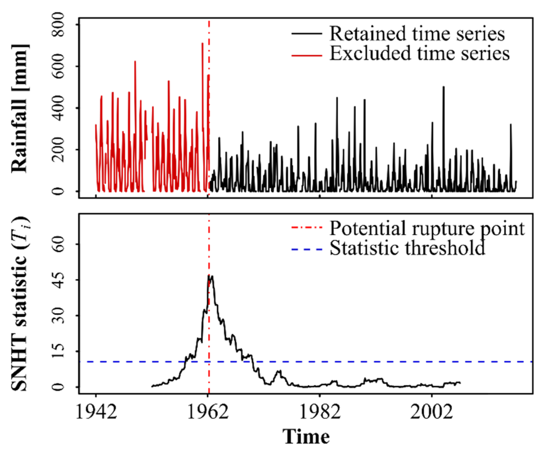
2.5.3. Trend Test and Change Point Detection

Trends in CRU TS rainfall and PET data were compared with trends in point-based data, considering the mean time series in each subregion. Series were pre-whitened (12-month moving average) in order to remove autocorrelation, and then linear trends were estimated through the least squares method [51]. The significance of the trend slopes was calculated through Student’s t-test (p < 0.01). Furthermore, the Pettitt change point detection test [52] was used to identify the exact year where a significant shift in the central tendency in the time series occurred, which was also compared between gridded and point-based measurements. When used in climate data, the Pettitt’s test indicates the approximate period when a significant change is observed in the mean behavior of a given meteorological variable. We also compared the slope of the trend in each grid of the CRU TS databases with point-based trends in observational data. In this case, we selected only one station per grid point with a significant trend (p < 0.01), and only stations with consistent data throughout the entire studied period.

3. Results

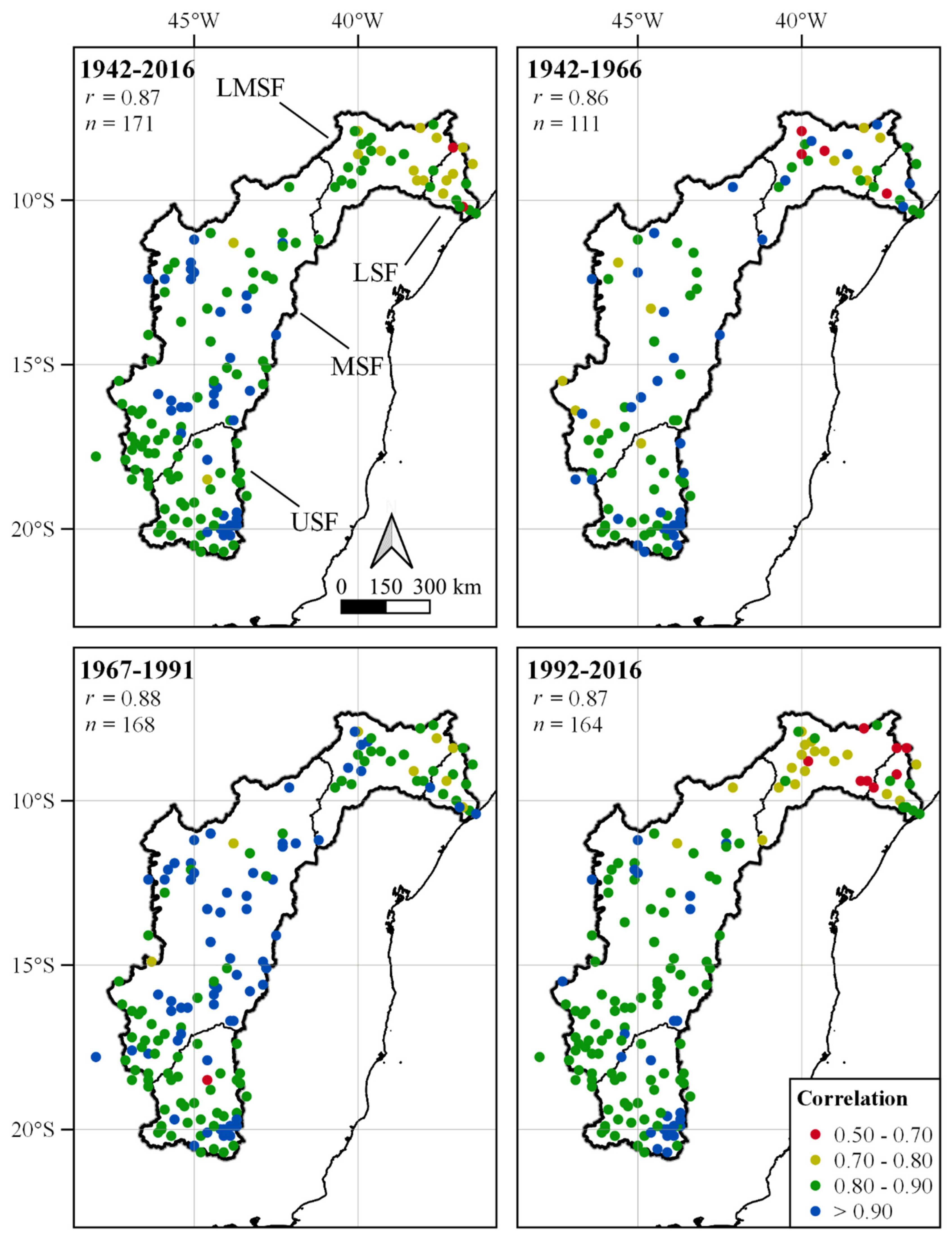
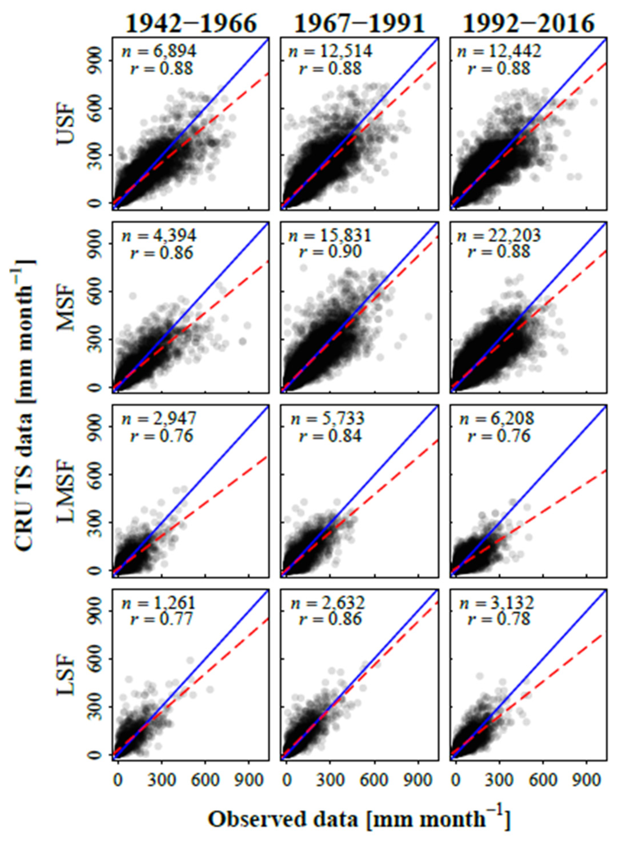
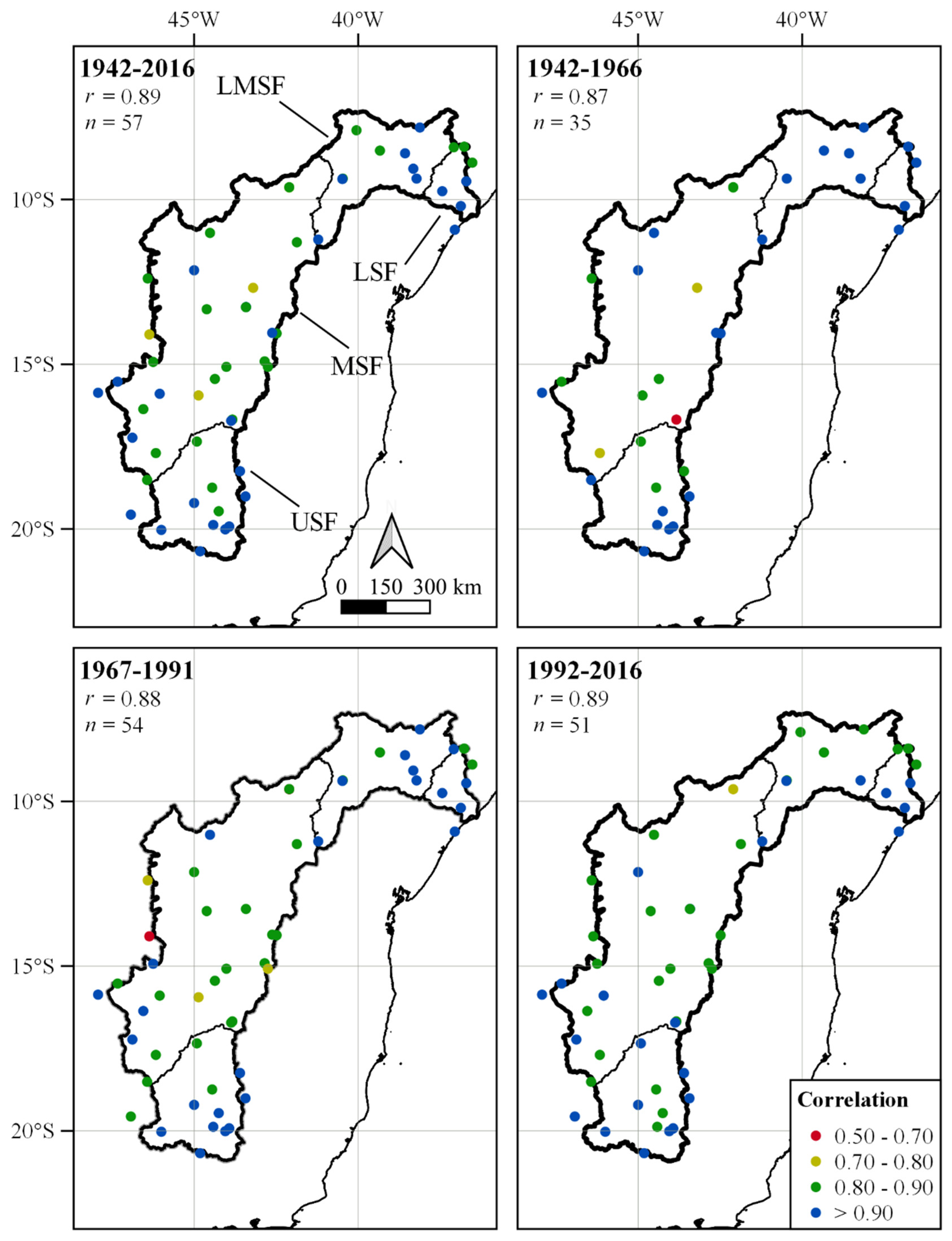
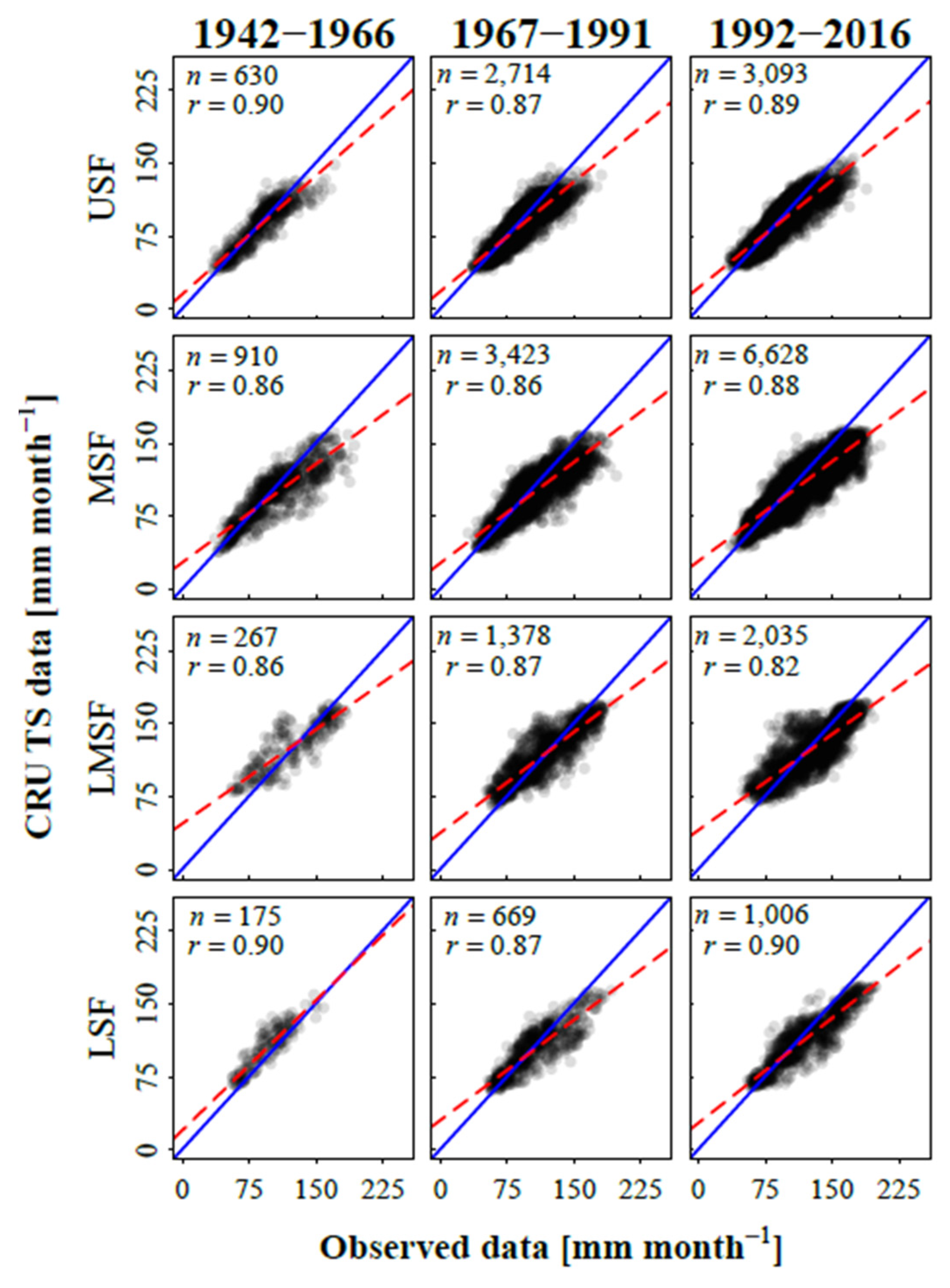
3.1. Overall Spatial and Temporal Performance

Figure 3 shows an overall strong correlation between CRU rainfall data and surface observations during the entire 75 years of the time series (r = 0.87). Individual correlations were mostly higher than 0.80 throughout the USF, MSF, and part of the LMSF. Only the transition zone between the LMSF (semiarid region) and the LSF (tropical coastal region) presented a few stations with which CRU data were weakly or moderately correlated (between 0.50 and 0.70).

Regarding the three 25-year periods, a noticeable increase in available stations can be observed from 1967 onwards. Overall, rainfall was best represented by the CRU TS dataset during the period from 1967–1991, when correlations below 0.80 were observed with only 12 out of the 168 stations. On the other hand, the most recent period (1992–2016) was when CRU TS data presented the weakest correlation (between 0.50 and 0.80) with almost all stations located in the LMSF and the LSF, although overall correlation was high (r = 0.87). Throughout the three periods, CRU TS data was mostly strongly correlated with observed data in the USF and MSF.

These results are further detailed in Figure 4, which shows the scatter plot of CRU TS rainfall data and observed data in each subregion of the SFW and for each 25-year period. It can be noted that in all plots CRU data seems to frequently underestimate higher monthly rainfall values. Another overall observation is that increasing the sample size did not necessarily lead to a better fit of the linear relationship between datasets.

As previously hinted in Figure 3, the highest slope coefficients of the scatter plot fit lines were found for the period from 1967–1991 (0.85; 0.90; 0.78; 0.91 for the USF, MSF, LMSF, and LSF, respectively). This means than in this period, the CRU TS rainfall estimates were less biased, and more correlated to observed data as evidenced by the correlation coefficients. The lowest slope coefficients (more frequent underestimations), however, were found in the most recent period, 1992–2016 (0.83; 0.81; 0.60; 0.72 for the USF, MSF, LMSF, and LSF, respectively), despite a larger available sample during these years. It is also worth mentioning that the differences between periods for the USF and MSF are much less prominent than for the LMSF and LSF.

Regarding PET values calculated using CRU TS temperature dataset, results appear to be more consistent both spatially and temporally, despite a few isolated poorly correlated stations in 1942–1966 and 1967–1991. Figure 5 shows that both in the 75-year period and in the three 25-year subperiods, most of the CRU TS data were mostly strongly correlated with available stations (r > 0.80). Furthermore, good relationships between datasets are found throughout the entire SFW, with no particular subregion presenting a weaker or stronger correlation pattern. This result was expected, since temperature, and therefore Thornthwaite’s PET, is less variable in the region.

The scatter plot between CRU TS temperature-derived PET and observed data (Figure 6) shows that the gridded dataset tends to more frequently underestimate high PET values, while low PET values are slightly overestimated. This pattern is observed across all analyzed 25-year periods and all subregions. It is also evident that low PET values in the LMSF (semiarid region) are more overestimated than in other regions. For example, the slope coefficient in the LMSF during 1992–2016 was 0.66, while in the USF, MSF, and LSF it was 0.74, 0.68, and 0.72, respectively.

Different to what was observed with rainfall data, correlation is higher during the first 25-year period in the USF and LSF (r = 0.90) with the regression line better fitting to the 1:1 ratio. During the two following periods, the slope of the scatter plot fit line does not seem to have changed much in any subregion, even with the increase in sample size. Nevertheless, the correlation coefficient in the last period (1992–2016) is similar or higher than in the first period (1942–1966) in all subregions, except for the LMSF.

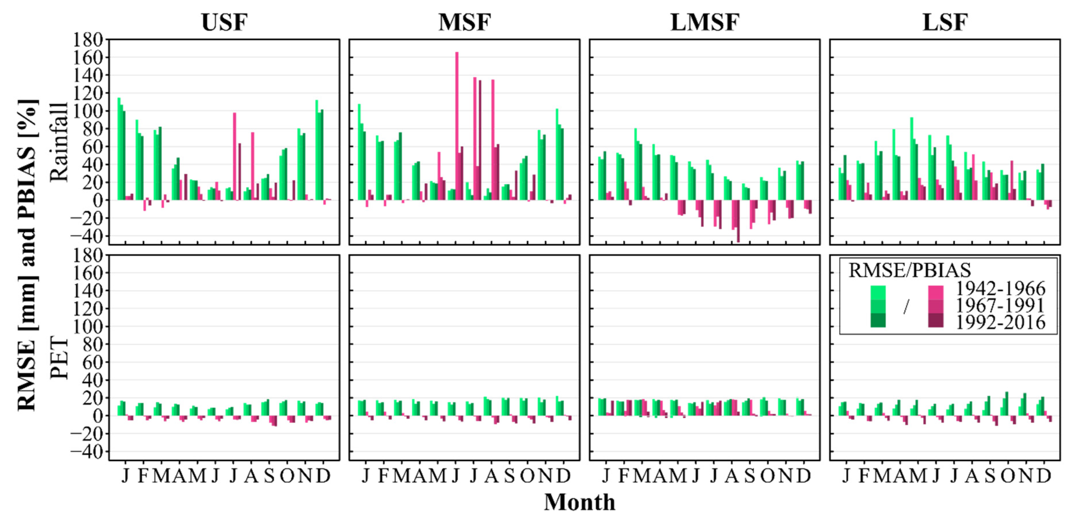
3.2. Seasonal Performance

The seasonal performance of the CRU TS datasets was assessed based on the analysis of monthly RMSE and PBIAS. Regarding rainfall estimates, Figure 7 shows that the RMSE generally improves in the most recent periods of the 75-year time series in all subregions. Since the RMSE is scale-dependent, higher values are found during the wet months if compared to dry months. In the LMSF and LSF, RMSE was lower than 68 mm in all months during the period from 1967 until 2016. During dry months, RMSE varied from 4 mm (August 1942–1966 in the MSF) to 34 mm (December 1942–1966 in the LSF).

Indeed, by analyzing the PBIAS of CRU TS rainfall data in relation to the observational dataset, one can notice high biases in the dry season. In the USF, mean rainfall is overestimated up to 97.6% (July 1942–1966), 75.9% (August 1942–1966), and 63.7% (July 1992–2016). A similar result is found in the MSF; despite a remarkable improvement in the most recent years, overestimations can reach up to 134.7% in July (1992–2016). In the semiarid region (LMSF), systematic underestimations of up to 47.5% (August 1992–2016) were found despite the low RMSE.

Regarding PET estimates, the behavior of monthly RMSE and PBIAS was more consistent and less important in all subregions and during all periods. RMSE ranged from 6.4 mm month⁻¹ in the LSF (August 1942–1966) to 26.8 mm month⁻¹ also in the LSF (October 1992–2016). PBIAS, on the other hand was higher in the LMSF, with overestimations of up to 11.4% in July (1942–1966).

Finally,

Table A1. Monthly mean (µ) ± standard deviation (σ) of CRU TS rainfall estimations and observed data in the: USF—upper; MSF—middle; LMSF—lower-middle; LSF—lower São Francisco watershed. The reliability of CRU TS estimates in each month is also shown based on whether monthly root mean square error is less than 50% of the mean observed value (where ✓ indicates reliable results and ✗ indicates nonreliable results).

Month	USF			MSF			LMSF			LSF
	CRU (µ ± σ)	Obs (µ ± σ)	Reliability	CRU (µ ± σ)	Obs (µ ± σ)	Reliability	CRU (µ ± σ)	Obs (µ ± σ)	Reliability	CRU (µ ± σ)	Obs (µ ± σ)	Reliability
1942–1966
Jan	281(±125)	276(±168)	✓	190(±116)	191(±162)	✗	63(±54)	68(±69)	✗	49(±41)	45(±48)	✗
Feb	177(±67)	211(±111)	✓	137(±73)	134(±93)	✗	75(±55)	73(±64)	✗	50(±40)	51(±56)	✗
Mar	151(±66)	160(±104)	✓	143(±92)	119(±105)	✗	114(±96)	107(±97)	✗	91(±76)	95(±81)	✗
Apr	62(±28)	47(±43)	✗	69(±49)	56(±57)	✗	76(±53)	87(±83)	✗	112(±84)	138(±109)	✗
May	30(±20)	27(±31)	✗	17(±19)	10(±15)	✗	39(±44)	48(±59)	✗	137(±122)	145(±114)	✗
Jun	12(±11)	9(±15)	✗	3(±7)	2(±6)	✗	29(±41)	36(±50)	✗	107(±84)	124(±83)	✗
Jul	13(±14)	7(±15)	✗	5(±11)	2(±7)	✗	22(±35)	30(±48)	✗	96(±76)	96(±72)	✗
Aug	9(±10)	5(±13)	✗	3(±7)	1(±4)	✗	13(±23)	16(±27)	✗	64(±56)	55(±48)	✗
Sep	36(±27)	30(±34)	✗	20(±24)	11(±19)	✗	7(±13)	12(±21)	✗	35(±42)	40(±45)	✗
Oct	116(±58)	110(±76)	✓	84(±62)	59(±62)	✗	12(±21)	17(±27)	✗	22(±23)	26(±37)	✗
Nov	208(±59)	186(±89)	✓	190(±88)	156(±102)	✗	37(±46)	42(±63)	✗	38(±37)	36(±39)	✗
Dec	298(±86)	306(±152)	✓	253(±120)	213(±141)	✓	48(±55)	58(±73)	✗	38(±44)	41(±50)	✗
1967–1991
Jan	266(±150)	250(±159)	✓	198(±151)	184(±143)	✓	79(±70)	74(±76)	✗	49(±42)	40(±47)	✗
Feb	158(±102)	151(±107)	✓	144(±110)	133(±105)	✓	90(±73)	83(±76)	✗	69(±55)	57(±61)	✗
Mar	156(±82)	146(±93)	✗	141(±92)	138(±109)	✓	136(±82)	135(±92)	✓	105(±67)	97(±70)	✗
Apr	68(±34)	66(±49)	✗	69(±46)	67(±58)	✗	92(±72)	95(±87)	✗	116(±79)	110(±88)	✓
May	30(±25)	28(±27)	✗	18(±23)	14(±19)	✗	43(±47)	48(±62)	✗	127(±117)	114(±113)	✗
Jun	14(±17)	12(±18)	✗	6(±14)	4(±9)	✗	30(±39)	30(±44)	✗	111(±88)	100(±75)	✗
Jul	14(±18)	14(±19)	✗	6(±17)	3(±8)	✗	29(±47)	29(±48)	✗	115(±102)	97(±80)	✗
Aug	14(±17)	13(±18)	✗	6(±13)	4(±10)	✗	11(±18)	14(±25)	✗	60(±51)	53(±45)	✗
Sep	47(±33)	44(±38)	✗	22(±22)	21(±25)	✗	9(±15)	11(±18)	✗	40(±43)	37(±41)	✗
Oct	119(±61)	121(±71)	✓	101(±67)	87(±65)	✗	16(±28)	16(±32)	✗	30(±39)	21(±31)	✗
Nov	218(±76)	218(±101)	✓	182(±86)	172(±98)	✓	27(±39)	34(±49)	✗	29(±32)	25(±37)	✗
Dec	279(±89)	273(±112)	✓	227(±127)	217(±132)	✓	55(±65)	58(±71)	✗	37(±44)	38(±49)	✗
1992–2016
Jan	275(±120)	260(±138)	✓	187(±115)	175(±129)	✓	88(±66)	82(±85)	✗	53(±39)	52(±74)	✗
Feb	140(±68)	151(±101)	✓	131(±72)	126(±96)	✗	75(±47)	82(±64)	✗	57(±34)	54(±57)	✗
Mar	162(±75)	172(±99)	✓	147(±83)	148(±107)	✗	106(±67)	105(±82)	✗	74(±45)	69(±71)	✗
Apr	79(±43)	59(±45)	✗	70(±48)	59(±55)	✗	70(±45)	63(±68)	✗	90(±57)	82(±75)	✗
May	29(±23)	28(±27)	✗	18(±17)	14(±20)	✗	41(±36)	38(±52)	✗	113(±88)	96(±92)	✗
Jun	11(±14)	10(±15)	✗	6(±14)	3(±8)	✗	26(±36)	27(±45)	✗	109(±83)	93(±82)	✗
Jul	9(±13)	5(±11)	✗	3(±6)	1(±5)	✗	24(±33)	22(±34)	✗	93(±64)	84(±65)	✗
Aug	11(±11)	10(±14)	✗	6(±9)	3(±9)	✗	9(±13)	12(±23)	✗	54(±43)	53(±47)	✗
Sep	51(±36)	43(±38)	✗	19(±19)	15(±21)	✗	8(±11)	6(±14)	✗	34(±33)	28(±34)	✗
Oct	115(±69)	95(±66)	✗	83(±59)	65(±60)	✗	11(±18)	15(±31)	✗	26(±26)	24(±35)	✗
Nov	213(±55)	214(±90)	✓	176(±71)	183(±98)	✓	25(±38)	33(±50)	✗	27(±25)	29(±42)	✗
Dec	295(±106)	299(±126)	✓	215(±104)	206(±114)	✓	47(±39)	54(±57)	✗	33(±23)	35(±49)	✗

(Appendix A, presented at the end of the manuscript before the references) shows the monthly observed and CRU TS rainfall mean (±standard deviation) for each 25-years period and each subregion. Furthermore, it indicates whether CRU TS estimates are reliable or not in each period based on the relative proportion of the RMSE in relation to the observed mean values. Overall, CRU TS rainfall estimates proved to be reliable in the wet season months of the USF and the MSF (approximately from October to March) in all period, except for 1942–1966 in the MSF. For the LMSF and the LSF, the RMSE analysis indicated that the monthly rainfall estimates of the CRU TS dataset are unreliable since the RMSE was higher than 50% of the observed mean values. This result, however, should be taken with care since the relative RMSE value in dry periods are expected to be high, although absolute differences may not be so remarkable. For example, in June 1942–1966, CRU TS rainfall was of 3 ± 7 mm in the MSF, while observed rainfall was of 2 ± 6 mm, which is obviously a reliable estimate despite the relative RMSE lower than 50%.

Similarly,

Table A2. Monthly mean (µ) ± standard deviation (σ) of CRU TS Thornthwaite’s potential evapotranspiration obtained through temperature estimations and observed data in the: USF—upper; MSF—middle; LMSF—lower-middle; LSF—lower São Francisco watershed. The reliability of CRU TS estimates in each month is also shown based on whether monthly root mean square error is less than 50% of the mean observed value (where ✓ indicates reliable results and ✗ indicates nonreliable results).

Month	USF			MSF			LMSF			LSF
	CRU (µ ± σ)	Obs (µ ± σ)	Reliability	CRU (µ ± σ)	Obs (µ ± σ)	Reliability	CRU (µ ± σ)	Obs (µ ± σ)	Reliability	CRU (µ ± σ)	Obs (µ ± σ)	Reliability
1942–1966
Jan	112(±9)	109(±16)	✓	121(±12)	116(±24)	✓	147(±14)	142(±30)	✓	146(±16)	140(±15)	✓
Feb	102(±9)	102(±15)	✓	111(±12)	105(±21)	✓	129(±13)	120(±28)	✓	128(±15)	127(±14)	✓
Mar	100(±9)	104(±15)	✓	116(±12)	114(±24)	✓	137(±15)	131(±32)	✓	138(±15)	134(±15)	✓
Apr	78(±9)	86(±13)	✓	100(±13)	102(±24)	✓	120(±13)	112(±29)	✓	115(±16)	115(±15)	✓
May	63(±7)	64(±11)	✓	88(±14)	88(±24)	✓	108(±12)	99(±27)	✓	105(±10)	101(±13)	✓
Jun	50(±6)	51(±9)	✓	72(±13)	71(±21)	✓	89(±10)	77(±18)	✓	87(±12)	85(±13)	✓
Jul	50(±6)	52(±8)	✓	70(±12)	71(±21)	✓	88(±13)	76(±20)	✓	81(±11)	79(±12)	✓
Aug	66(±8)	71(±16)	✓	86(±12)	89(±26)	✓	92(±12)	88(±21)	✓	85(±12)	81(±10)	✓
Sep	81(±10)	92(±20)	✓	110(±14)	112(±28)	✓	112(±16)	110(±26)	✓	95(±12)	91(±10)	✓
Oct	99(±12)	104(±23)	✓	124(±15)	128(±31)	✓	143(±18)	135(±32)	✓	120(±13)	114(±13)	✓
Nov	97(±10)	108(±22)	✓	116(±14)	121(±30)	✓	144(±14)	139(±31)	✓	132(±16)	123(±13)	✓
Dec	105(±9)	113(±18)	✓	119(±13)	120(±27)	✓	153(±16)	146(±31)	✓	143(±16)	134(±15)	✓
1967–1991
Jan	114(±11)	120(±20)	✓	124(±13)	123(±22)	✓	146(±13)	142(±27)	✓	145(±16)	138(±23)	✓
Feb	105(±9)	110(±18)	✓	114(±12)	111(±21)	✓	127(±13)	123(±25)	✓	126(±16)	123(±20)	✓
Mar	106(±10)	113(±17)	✓	120(±12)	118(±20)	✓	134(±15)	131(±28)	✓	137(±16)	131(±22)	✓
Apr	83(±10)	89(±17)	✓	104(±13)	103(±19)	✓	120(±13)	116(±25)	✓	115(±17)	116(±23)	✓
May	67(±8)	70(±13)	✓	92(±14)	92(±20)	✓	108(±13)	104(±25)	✓	106(±11)	106(±25)	✓
Jun	53(±7)	56(±10)	✓	76(±14)	76(±19)	✓	89(±10)	86(±20)	✓	88(±13)	89(±25)	✓
Jul	53(±7)	56(±10)	✓	74(±13)	76(±18)	✓	88(±14)	82(±19)	✓	82(±13)	88(±28)	✓
Aug	68(±8)	73(±13)	✓	90(±13)	96(±22)	✓	95(±12)	94(±23)	✓	88(±13)	93(±29)	✓
Sep	77(±9)	87(±17)	✓	110(±15)	114(±24)	✓	116(±17)	115(±27)	✓	97(±13)	103(±31)	✓
Oct	98(±11)	106(±19)	✓	126(±16)	129(±25)	✓	144(±17)	141(±29)	✓	123(±14)	123(±27)	✓
Nov	103(±9)	108(±18)	✓	120(±14)	120(±23)	✓	145(±14)	146(±27)	✓	134(±16)	130(±23)	✓
Dec	109(±10)	115(±18)	✓	123(±14)	121(±22)	✓	154(±16)	152(±28)	✓	144(±16)	137(±23)	✓
1992–2016
Jan	120(±11)	126(±21)	✓	131(±13)	136(±22)	✓	150(±13)	147(±27)	✓	149(±17)	150(±23)	✓
Feb	110(±11)	115(±19)	✓	119(±13)	123(±21)	✓	131(±13)	130(±23)	✓	130(±16)	134(±20)	✓
Mar	109(±11)	114(±18)	✓	125(±13)	127(±22)	✓	140(±14)	140(±26)	✓	142(±15)	145(±22)	✓
Apr	90(±10)	95(±15)	✓	112(±13)	116(±21)	✓	125(±14)	126(±27)	✓	120(±18)	131(±22)	✓
May	68(±8)	70(±12)	✓	97(±15)	101(±23)	✓	113(±13)	115(±28)	✓	110(±12)	120(±25)	✓
Jun	54(±6)	56(±11)	✓	79(±15)	82(±19)	✓	91(±10)	90(±23)	✓	90(±15)	101(±26)	✓
Jul	57(±6)	59(±12)	✓	81(±14)	83(±19)	✓	93(±14)	87(±23)	✓	85(±15)	99(±30)	✓
Aug	72(±9)	75(±16)	✓	96(±14)	102(±21)	✓	97(±12)	97(±27)	✓	90(±14)	106(±34)	✓
Sep	85(±12)	96(±21)	✓	120(±16)	130(±23)	✓	120(±18)	119(±28)	✓	101(±14)	118(±33)	✓
Oct	108(±14)	118(±24)	✓	138(±16)	149(±24)	✓	148(±17)	144(±27)	✓	128(±14)	138(±31)	✓
Nov	106(±10)	113(±22)	✓	126(±15)	133(±24)	✓	149(±14)	149(±26)	✓	138(±16)	144(±25)	✓
Dec	117(±11)	122(±20)	✓	131(±14)	136(±23)	✓	159(±15)	154(±27)	✓	149(±15)	154(±23)	✓

(Appendix A, presented at the end of the manuscript before the references) shows the monthly observed and CRU TS Thornthwaite’s PET mean (± standard deviation) for each 25-year period and each subregion. In this case, the analysis of the RMSE indicated that the CRU TS product is reliable in all months, during the entire 75-years period and in all subregions.

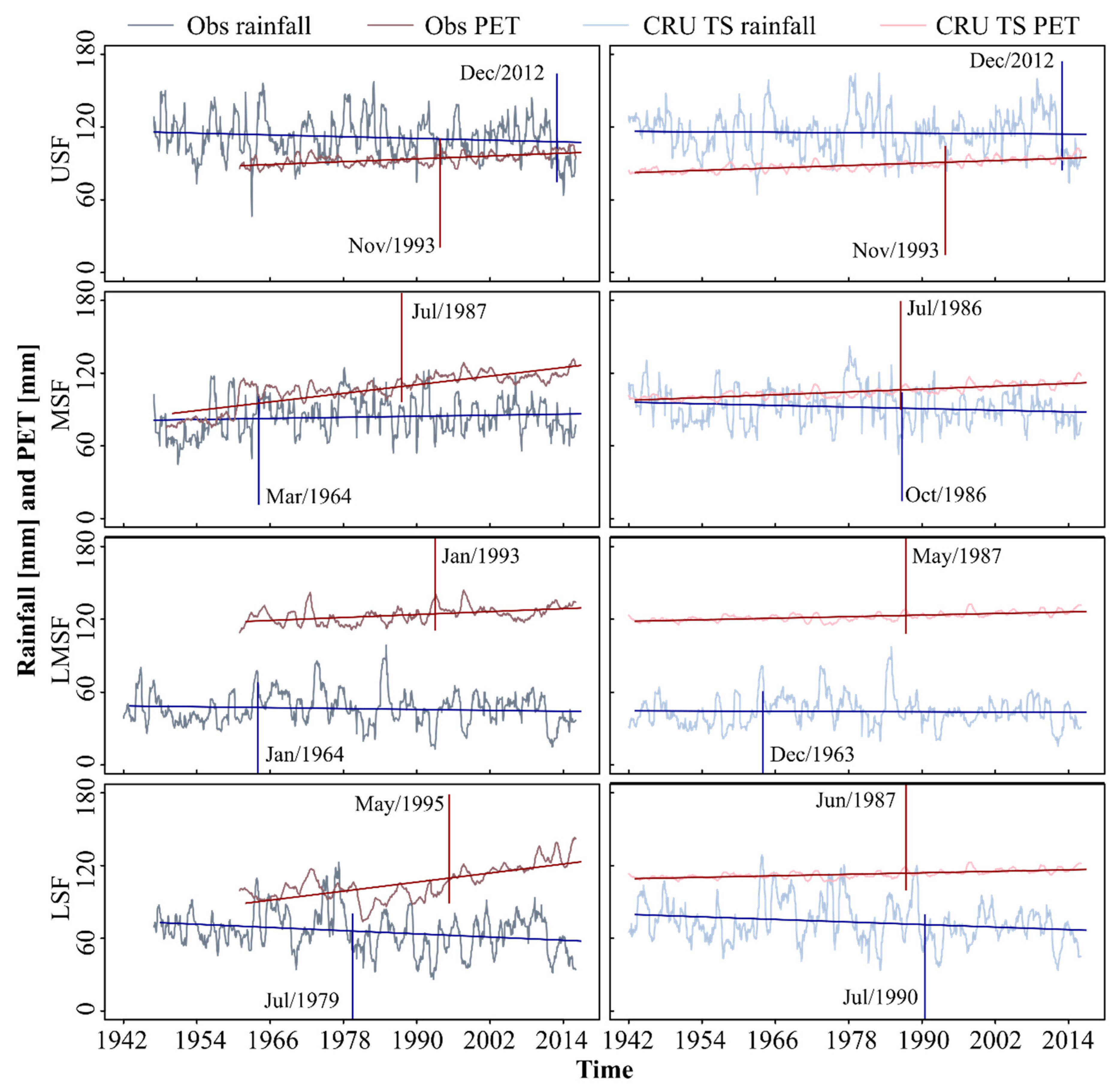
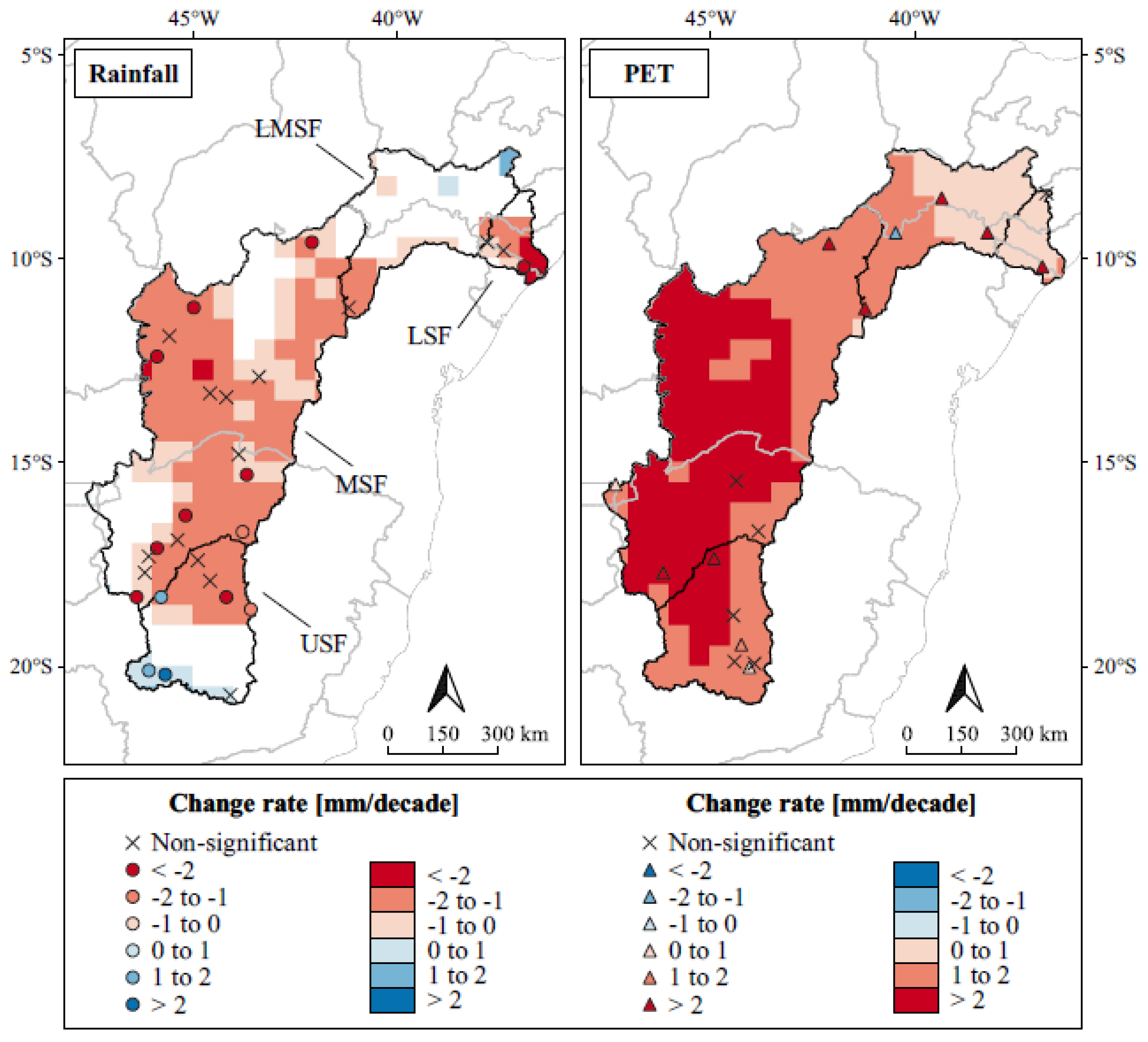
3.3. Trends and Change-Point Comparisons

Firstly, we compared the trends and change-points detected in the smoothed monthly mean time series of rainfall and PET derived from the CRU TS dataset and observational data (Figure 8). For the USF, the same change-points were identified in both datasets: December 2012 and November 1993 for rainfall and PET, respectively. Furthermore, significant decreasing trends were found (

Table 2. Summary of the trends and change-point detection analysis for observed and CRU TS rainfall and Thornthwaite’s potential evapotranspiration data in the: USF—upper; MSF—middle; LMSF—lower-middle; LSF—lower São Francisco watershed. Statistically significant trend slopes and change-points (α = 1%) are highlighted in italic.

Subregion	Change Point	Period	Annual Mean (mm)	Slope (mm/Decade)
USF
Obs rainfall	Dec/2012	Jan/1942–Dec/2016	1339	−1
		Jan/1942–Dec/2012	1355	0
		Dec/2012–Dec/2016	1056	−14
CRU TS rainfall	Dec/2012	Jan/1942–Dec/2016	1383	−1
		Jan/1942–Dec/2012	1397	0
		Dec/2012–Dec/2016	1120	−17
Obs PET	Nov/1993	Jan/1942–Dec/2016	1123	2
		Jan/1942–Nov/1993	1092	1
		Nov/1993–Dec/2016	1165	3
CRU TS PET	Nov/1993	Jan/1942–Dec/2016	1063	2
		Jan/1942–Nov/1993	1036	1
		Nov/1993–Dec/2016	1122	3
MSF
Obs rainfall	Mar/1964	Jan/1942–Dec/2016	1006	1
		Jan/1942–Mar/1964	913	11
		Mar/1964–Dec/2016	1035	−2
CRU TS rainfall	Oct/1986	Jan/1942–Dec/2016	1103	−1
		Jan/1942–Oct/1986	1138	0
		Oct/1986–Dec/2016	1059	0
Obs PET	Jul/1987	Jan/1942–Dec/2016	1275	6
		Jan/1942–Jul/1987	1171	8
		Jul/1987–Dec/2016	1406	2
CRU TS PET	Jul/1986	Jan/1942–Dec/2016	1258	2
		Jan/1942–Jul/1986	1219	1
		Jul/1986–Dec/2016	1312	3
LMSF
Obs rainfall	Jan/1964	Jan/1942–Dec/2016	557	0
		Jan/1942–Jan/1964	520	−4
		Jan/1964–Dec/2016	572	−3
CRU TS rainfall	Dec/1963	Jan/1942–Dec/2016	528	0
		Jan/1942–Dec/1963	475	−1
		Dec/1963–Dec/2016	552	−3
Obs PET	Jan/1993	Jan/1942–Dec/2016	1484	2
		Jan/1942–Jan/1993	1445	0
		Jan/1993–Dec/2016	1535	−1
CRU TS PET	May/1987	Jan/1942–Dec/2016	1467	1
		Jan/1942–May/1987	1444	0
		May/1987–Dec/2016	1500	1
LSF
Obs rainfall	Jul/1979	Jan/1942–Dec/2016	785	−2
		Jan/1942–Jul/1979	866	5
		Jul/1979–Dec/2016	720	1
CRU TS rainfall	Jul/1990	Jan/1942–Dec/2016	878	−1
		Jan/1942–Jul/1990	928	2
		Jul/1990–Dec/2016	803	1
Obs PET	May/1995	Jan/1942–Dec/2016	1269	6
		Jan/1942–May/1995	1162	−1
		May/1995–Dec/2016	1427	11
CRU TS PET	Jun/1987	Jan/1942–Dec/2016	1355	1
		Jan/1942–Jun/1987	1333	0
		Jun/1987–Dec/2016	1387	1

) for both the entire rainfall time series (−1 mm decade⁻¹) and from December 2012 to 2016 (−14 and −17 mm decade⁻¹ for observed and CRU TS data, respectively).

Regarding PET data, significant increasing trends were found in both datasets and in all portions of the time series (Figure 8 and Table 2). Indeed, the change rate in PET increased from 1 mm decade⁻¹ until 1993 to 3 mm decade⁻¹ in the last 25 years of the studied period. The mean PET in the two sections of the time series increased from 1092 mm (observational) and 1036 mm (CRU TS) to 1165 mm (observational) and 1122 mm (CRU TS).

In the MSF, an important change in behavior was identified by Pettitt’s test in the observed time series in March 1964 (Figure 8 and Table 2). Indeed, rainfall values increased after this year but subsequently presented a significant decreasing trend of −2 mm decade⁻¹. For CRU TS rainfall data, a significant change-point was detected in October 1986, while the decreasing trend was significant only when considering the entire time series (−1 mm decade⁻¹). Regarding PET in the MSF, similar change-points were detected in the two datasets: July 1987 (observations) and July 1986 (CRU TS). Furthermore, significant increasing trends were found in both datasets, although in the observational data the overall change rate was of 8 mm decade⁻¹ compared to only 2 mm decade⁻¹ for the CRU TS time series.

Still regarding Figure 8 and Table 2, also similar change-points were found in the LMSF rainfall time series: January 1964 and December 1963, for the observations and CRU TS estimates, respectively. Both portions of the time series presented significant decreasing trends: −4 and −3 mm decade⁻¹ for the observational data and −1 and −2 mm decade⁻¹ for CRU TS data. Therefore, rainfall derived from the CRU TS dataset appears to decrease slightly smoother than observed data. Regarding PET data in the LMSF, nonsignificant change-points were found, while a significant overall increasing trend was found in both datasets.

Finally, significant change-points at different periods were detected in the LSF (Figure 8 and Table 2): July 1979 and May 1995, for observed and CRU TS rainfall data, respectively. In these series, significant decreasing trends of −2 and −1 mm decade⁻¹ were found with a mean annual rainfall of 785 mm and 878 mm for observational and CRU TS data, respectively. At the same time, a remarkable significant increasing trend of 6 mm decade⁻¹ was found for observed PET data. This increase reached up to 11 mm decade⁻¹ in the period from May 1995 until the end of the series. CRU TS derived PET also presented significant increasing trends, but with a much less important change rate (1 mm decade⁻¹).

The spatial distribution of the significant trend slopes (p < 0.01) of CRU TS data is shown in Figure 9. For rainfall, negative trends are found in most part of the MSF, LSF and the northern portion of the USF. Additionally, positive trends are found in the southern portion of the USF. Overall, these results are similar to what was found with observed data, which also indicated negative trends in the same regions of the SFW, although with higher change rates. Furthermore, CRU TS data featured significant rainfall trends in large areas of the basin, while point-based significant trends are more heterogeneous and sparser.

Regarding Thonrthwaite’s PET derived from the CRU TS dataset, significant trends were found in the entire SFW, indicating an increase in the atmospheric demand for water. Indeed, observational data was also mostly significant, mainly in the LMSF and LSF while some stations in the MSF and USF presented non-significant trends. One station at the LMSF, near the Sobradinho reservoir, presented negative PET trend, which was not captured by the CRU TS dataset. The magnitude of the change rate is also stronger in observed data than in CRU TS data, particularly in the LMSF and the LSF.

4. Discussion

In the first part of the study we assessed the overall spatial and temporal performance of the CRU TS dataset in representing monthly rainfall and PET (estimated from temperature data) over the SFW.

CRU TS rainfall data presented weaker correlation with observed data in the LMSF and the LSF, which is probably associated with the high spatial and temporal variability of precipitation in these regions. The LMSF is entirely located in the semiarid region of Brazil while the LSF comprises a transition zone between a semiarid environment and the coastal zone, with a more humid climate [30]. Thus, it is expected that interpolated datasets with relatively large spatial resolutions such as the CRU TS (~57 km) will perform worse in these regions. Previous studies have already reported a poorer performance of gridded datasets in regions of high rainfall variability such as semiarid zones in Pakistan [53]. PET data, on the other hand, presented more consistent results in spatial terms. Indeed, temperature and consequently Thornthwaite’s PET spatial and temporal patterns are less variable [54,55].

The scatter plot between data showed that rainfall CRU TS data generally underestimate higher rainfall and PET values, while low PET values are usually overestimated. This is probably associated with the smoothing of data which is inherent to interpolation techniques used to produce gridded datasets [6,56].

Results showed that the best correlations between data were found in the period from 1967–1991, while the most recent period (1992–2016) presented slightly worst correlations. There are two potential explanations for this fact. Firstly, the density of the contributing stations with at least 75% of observations per decade for the development of the CRU TS product was higher in the second half of the 20th century than in the first decades of the 21st century [13]. Thus, it is expected that a higher density of stations provides better interpolated estimates when comparing with point-based observations. Another explanation is associated with the aforementioned characteristic of gridded datasets of usually performing worse over semiarid and drier regions. The period from 1992–2016 comprised the worst drought event (2012–2016) registered in the semiarid region of Brazil [57,58], which may have also contributed to the poorer performance of the algorithm in this 25-years period, especially in the LMSF and LSF.

The seasonal performance of the CRU TS datasets was assessed based on the monthly RMSE and PBIAS. Since the RMSE is scale-dependent, it was proportional to the overall magnitude of the assessed variables. Thus, higher rainfall RMSE are found during the wet season, while for PET it is rather stable throughout the year. The PBIAS, on the other hand, is much more sensitive to lower values (dry season) but indicates the direction of the monthly bias (underestimation or overestimation of observed values). Thus, high PBIAS values should be interpreted with caution for the dry season, while high RMSE values should be interpreted with caution for the wet season.

Results showed that CRU TS data generally overestimates rainfall during the dry season in the USF and MSF, while during the wet season estimations are reliable (RMSE < 50% of observed mean value). For Thornthwaite’s PET, CRU TS slightly underestimates (maximum PBIAS of −10%) observations during all months in the USF, MSF, and LSF, although the estimates are reliable. Therefore, when using CRU TS data to monitor temperature and temperature-derived PET, one should note that actual atmospheric demand for water is slightly higher in these regions. In the LMSF, however, results are the opposite, with actual PET being slightly slower than CRU TS derived PET.

Monthly mean values of rainfall and PET derived from the CRU TS were comparable to those observed in surface stations. In the USF, higher rainfall rates were observed in the austral autumn and summer (October to March), mainly due to the development of the South Atlantic Convergence Zone in the central portion of South America, encompassing the western and southern SFW [30,59,60]. In the MSF, a similar pattern was observed, but with smaller rainfall rates since the region is larger and comprises the transition zone between the humid subtropical climate and the semiarid.

In the northern portion of the SFW, the LMSF is under the influence of a semiarid climate, where rainfall is modulated mainly by the position of the Intertropical Convergence Zone (ITCZ) from February to May [30,61], producing rainfall extreme events in that region [24]. The LSF, on the other hand, presents a rainfall regime typical of coastal zones in the Northeast Brazil (Köppen’s As–tropical with dry summer), with important rain events occurring from March to July, mainly due to the ITCZ, sea breezes, and the propagation of easterly wave disturbances [30,62,63]. Regarding PET, seasonal variations are similar in all subregions of the SFW, although lower values are found in the higher latitudes of the basin (USF and MSF).

For the assessment of long-term monitoring of the two components of the climatic water balance, trends and change-points of CRU TS data were compared to observed data. Regarding regional mean time series, a general decreasing trend in rainfall and increasing trend in PET was observed in all subregions. Trends in both datasets presented the same sign, although observed data presented higher slopes, indicating that the actual balance between precipitation and PET may favor higher atmospheric demand for water in the future. In fact, the study by Marengo et al. [34] already projected an increase of up to 1.5 °C in temperature and a decrease of up to 20% in rainfall over the SFW until 2040. These results were corroborated by De Jong et al. [64]. The smaller slopes in CRU TS data trends may also be related to the smoothing of data due to the interpolation procedure, which can be clearly visualized in Figure 8.

Remarkable positive trend slopes for PET time series were found in the MSF and LSF (6 mm decade⁻¹). Curiously, these are the regions surrounding the semiarid portion of the basin (LMSF), which may indicate an expansion of arid zones towards regions under more humid climates. Indeed, Dubreuil et al. [37] recently detected an expansion of the areas under semiarid climate in Brazil.

These results are further confirmed by the spatial distribution of CRU TS and point-based trend slopes presented in Figure 9. CRU TS data shows clear significant decreasing trends in rainfall over the MSF and LSF and an increase in the atmospheric demand for water throughout the entire watershed. The significance of point-based measures is more heterogeneous, which has been previously evidenced by Bezerra et al. [30]. It is also important to note that the negative rainfall trends observed in the LSF would not necessarily impact water availability in the São Francisco river, since it is located near its mouth. These changes, however, may influence the occurrence of rainfall extreme events in the region, which has been detected in previous studies [60].

Regarding point-based PET trends, a single isolated station presented a decreasing trend. In fact, this station is located downstream of the Sobradinho reservoir and the many irrigated perimeters that developed after the construction of the dam in the early 1980s. Previous studies have already assessed PET trends in this particular region, finding similar results and suggesting that the massive extension of the dam’s lake and the irrigated perimeters might have influenced local climate [33].

5. Conclusions

This study presented a thorough assessment of rainfall and PET (calculated through temperature data) derived from the CRU TS dataset in the SFW, an extremely important basin in Brazil that lacks long-term consistent observed data with good spatial coverage for these variables. The study comprised time series of 75 years (1942–2016), and the evaluation was carried out also considering three 25-years period (1942–1966, 1967–1991, and 1992–2016) and four subregions of the basin (USF, MSF, LMSF, LSF) with different climate characteristics.

Overall, CRU TS data was strongly correlated with observational data, with maximum r equal to 0.88 in 1967–1991 for rainfall data and 0.89 in 1992–2016 for PET data. The spatial distribution of correlations indicated that the poorest performances (r ranging from 0.50 to 0.80) occurred in the LMSF and LSF regions, which are characterized by a semiarid climate and the transition to a humid coastal zone.

The evaluation of monthly estimates showed that estimations of Thornthwaite’s PET obtained through CRU TS temperature data are reliable (RMSE < 50% of observed mean) in all months and in all subregions. Regarding rainfall data, CRU TS data was reliable for estimations derived during the wet months in the USF and MSF. In either case, results derived from analysis using these products must always be interpreted with caution. In fact, the present study strongly advocates that more in-depth assessment procedures should be carried out before using any gridded product for meteorological variables. Understanding the strengths and limitations of these datasets should be a first step in every study proposing their use.

The trends detected in both datasets pointed towards the same direction: increasing PET in all subregions and decreasing rainfall mostly in the MSF and the LSF, the areas surrounding the semiarid portion of the SFW. However, the slope of the trends in observed data was steeper than in CRU TS data.

In general, CRU TS data are consistent with observed data and their use should be encouraged, given that the actual conditions of available observed data in the region (as evidenced in Supplementary Figures S1 and S2) seriously limits consistent long-term hydroclimatological studies. However, the assessment provided in the present study should always be taken into consideration when using CRU TS rainfall and temperature data over the SFW.

References

1. Nelson, G.C.; Valin, H.; Sands, R.D.; Havlík, P.; Ahammad, H.; Deryng, D.; Kyle, P. Climate change effects on agriculture: Economic responses to biophysical shocks. Proc. Natl. Acad. Sci. USA 2014, 111, 3274–3279. [Google Scholar] [CrossRef] [Green Version]
2. Rosenzweig, C.; Elliott, J.; Deryng, D.; Ruane, A.C.; Müller, C.; Arneth, A.; Neumann, K. Assessing agricultural risks of climate change in the 21st century in a global gridded crop model intercomparison. Proc. Natl. Acad. Sci. USA 2014, 111, 3268–3273. [Google Scholar] [CrossRef] [Green Version]
3. Arora, N.K. Impact of climate change on agriculture production and its sustainable solutions. Environ. Sustain. 2019, 2, 95–96. [Google Scholar] [CrossRef] [Green Version]
4. Folberth, C.; Khabarov, N.; Balkovič, J.; Skalský, R.; Visconti, P.; Ciais, P.; Obersteiner, M. The global cropland-sparing potential of high-yield farming. Nat. Sustain. 2020, 3, 281–289. [Google Scholar] [CrossRef]
5. Huang, J.; Ji, M.; Xie, Y.; Wang, S.; He, Y.; Ran, J. Global semi-arid climate change over last 60 years. Clim. Dyn. 2016, 46, 1131–1150. [Google Scholar] [CrossRef] [Green Version]
6. Henn, B.; Newman, A.J.; Livneh, B.; Daly, C.; Lundquist, J.D. An assessment of differences in gridded precipitation datasets in complex terrain. J. Hydrol. 2018, 556, 1205–1219. [Google Scholar] [CrossRef]
7. Shi, H.; Li, T.; Wei, J. Evaluation of the gridded CRU TS precipitation dataset with the point raingauge records over the Three-River Headwaters Region. J. Hydrol. 2017, 548, 322–332. [Google Scholar] [CrossRef] [Green Version]
8. Michot, V.; Vila, D.; Arvor, D.; Corpetti, T.; Ronchail, J.; Funatsu, B.M.; Dubreuil, V. Performance of TRMM TMPA 3B42 V7 in replicating daily rainfall and regional rainfall regimes in the Amazon basin (1998–2013). Remote Sens. 2018, 10, 1879. [Google Scholar] [CrossRef] [Green Version]
9. Alemayehu, T.; van Griensven, A.; Bauwens, W. Evaluating CFSR and WATCH data as input to SWAT for the estimation of the potential evapotranspiration in a data-scarce Eastern-African catchment. J. Hydrol. Eng. 2016, 21, 05015028. [Google Scholar] [CrossRef]
10. Harris, I.; Jones, P.D.; Osborn, T.J.; Lister, D.H. Updated high-resolution grids of monthly climatic observations—The CRU TS3.10 Dataset. Int. J. Clim. 2014, 34, 623–642. [Google Scholar] [CrossRef] [Green Version]
11. Wagner, P.D.; Fiener, P.; Wilken, F.; Kumar, S.; Schneider, K. Comparison and evaluation of spatial interpolation schemes for daily rainfall in data scarce regions. J. Hydrol. 2012, 464–465, 388–400. [Google Scholar] [CrossRef]
12. Chen, M.; Shi, W.; Xie, P.; Silva, V.B.S.; Kousky, V.E.; Higgins, R.W.; Janowiak, J.E. Assessing objective techniques for gauge-based analyses of global daily precipitation. J. Geophys. Res. Atmos. 2008, 113, 1–13. [Google Scholar] [CrossRef]
13. Harris, I.; Osborn, T.J.; Jones, P.; Lister, D. Version 4 of the CRU TS monthly high-resolution gridded multivariate climate dataset. Sci. Data 2020, 7, 1–18. [Google Scholar] [CrossRef] [Green Version]
14. Schamm, K.; Ziese, M.; Becker, A.; Finger, P.; Meyer-Christoffer, A.; Schneider, U.; Stender, P. Global gridded precipitation over land: A description of the new GPCC First Guess Daily product. Earth Syst. Sci. Data 2014, 6, 49–60. [Google Scholar] [CrossRef] [Green Version]
15. Funk, C.C.; Peterson, P.J.; Landsfeld, M.F.; Pedreros, D.H.; Verdin, J.P.; Rowland, J.D.; Verdin, A.P. A Quasi-Global Precipitation Time Series for Drought Monitoring. 2014. Available online: https://pubs.er.usgs.gov/publication/ds832 (accessed on 23 June 2020).
16. Huffman, G.J.; Bolvin, D.T. TRMM and Other Data Precipitation Data Set Documentation. 2015. Available online: https://pmm.nasa.gov/sites/default/files/document_files/3B42_3B43_doc_V7.pdf (accessed on 23 June 2020).
17. Ma, L.; Zhang, T.; Frauenfeld, O.W.; Ye, B.; Yang, D.; Qin, D. Evaluation of precipitation from the ERA-40, NCEP-1, and NCEP-2 reanalyses and CMAP-1, CMAP-2, and GPCP-2 with ground-based measurements in China. J. Geophys. Res. Atmos. 2009, 114, 1–20. [Google Scholar] [CrossRef]
18. Salvacion, A.R.; Magcale-Macandog, D.B.; Cruz, P.C.S.; Saludes, R.B.; Pangga, I.B.; Cumagun, C.J.R. Evaluation and spatial downscaling of CRU TS precipitation data in the Philippines. Model Earth Syst. Environ. 2018, 4, 891–898. [Google Scholar] [CrossRef]
19. Prömmel, K.; Geyer, B.; Jones, J.M.; Widmann, M. Evaluation of the skill and added value of a reanalysis-driven regional simulation for Alpine temperature. Int. J. Clim. 2010, 30, 760–773. [Google Scholar] [CrossRef] [Green Version]
20. Jones, P.D.; Harpham, C.; Harris, I.; Goodess, C.M.; Burton, A.; Centella-Artola, A.; Joslyn, O. Long-term trends in precipitation and temperature across the Caribbean. Int. J. Clim. 2016, 36, 3314–3333. [Google Scholar] [CrossRef] [Green Version]
21. Malsy, M.; aus der Beek, T.; Flörke, M. Evaluation of large-scale precipitation data sets for water resources modelling in Central Asia. Environ. Earth Sci. 2015, 73, 787–799. [Google Scholar] [CrossRef]
22. Thorne, P.W.; Donat, M.G.; Dunn, R.J.H.; Williams, C.N.; Alexander, L.V.; Caesar, J.; Menne, M.J. Reassessing changes in diurnal temperature range: Intercomparison and evaluation of existing global data set estimates. J. Geophys. Res. Atmos. 2016, 121, 5138–5158. [Google Scholar] [CrossRef] [Green Version]
23. Paredes-Trejo, F.J.; Barbosa, H.A.; Kumar, T.V.L. Validating CHIRPS-based satellite precipitation estimates in Northeast Brazil. J. Arid. Environ. 2017, 139, 26–40. [Google Scholar] [CrossRef]
24. Rodrigues, D.T.; Gonçalves, W.A.; Spyrides, M.H.C.; Santos e Silva, C.M. Spatial and temporal assessment of the extreme and daily precipitation of the Tropical Rainfall Measuring Mission satellite in Northeast Brazil. Int. J. Remote Sens. 2020, 41, 549–572. [Google Scholar] [CrossRef]
25. Xavier, A.C.; King, C.W.; Scanlon, B.R. Daily gridded meteorological variables in Brazil (1980-2013). Int. J. Clim. 2016, 2659, 2644–2659. [Google Scholar] [CrossRef] [Green Version]
26. Mutti, P.R.; de Abreu, L.P.; de MB Andrade, L.; Spyrides, M.H.C.; Lima, K.C.; de Oliveira, C.P.; Bezerra, B.G. A detailed framework for the characterization of rainfall climatology in semiarid watersheds. Theor. Appl. Climatol. 2020, 139, 109–125. [Google Scholar] [CrossRef]
27. Mudelsee, M. Trend analysis of climate time series: A review of methods. Earth-Sci. Rev. 2019, 190, 310–322. [Google Scholar] [CrossRef]
28. Mendes, L.A.; de Barros, M.T.L.; Zambon, R.C.; Yeh, W.W.G. Trade-off analysis among multiple water uses in a hydropower system: Case of São Francisco River Basin, Brazil. J. Water Resour. Plan Manag. 2015, 141, 04015014. [Google Scholar] [CrossRef]
29. Koch, H.; Selge, F.; de Azevedo, J.R.G.; da Silva, G.N.S.; Siegmund-Schultze, M.; Hattermann, F.F. Reservoir operation and environmental water demand: Scenarios for the Sub-Middle and Lower São Francisco River basin, Brazil. Ecohydrology 2018, 11, e2026. [Google Scholar] [CrossRef]
30. Bezerra, B.G.; Silva, L.L.; Santos ESilva, C.M.; de Carvalho, G.G. Changes of precipitation extremes indices in São Francisco River Basin, Brazil from 1947 to 2012. Appl. Clim. 2019, 135, 565–576. [Google Scholar] [CrossRef]
31. Marques, É.T.; Gunkel, G.; Sobral, M.C. Management of tropical river basins and reservoirs under water stress: Experiences from Northeast Brazil. Environments 2019, 6, 62. [Google Scholar] [CrossRef] [Green Version]
32. Stolf, R.; de Piedade, S.M.; Silva, J.R.D.; da Silva, L.C.; Maniero, M.Â. Water transfer from São Francisco river to semiarid northeast of Brazil: Technical data, environmental impacts, survey of opinion about the amount to be transferred. Eng. Agríc. 2012, 32, 998–1010. [Google Scholar] [CrossRef] [Green Version]
33. Cabral Júnior, J.B.; Santos e Silva, C.M.; de Almeida, H.A.; Bezerra, B.G.; Spyrides, M.H.C. Detecting linear trend of reference evapotranspiration in irrigated farming areas in Brazil’s semiarid region. Appl. Clim. 2019, 138, 215–225. [Google Scholar] [CrossRef]
34. Marengo, J.A.; Chou, S.C.; Kay, G.; Alves, L.M.; Pesquero, J.F.; Soares, W.R.; Chagas, D.J. Development of regional future climate change scenarios in South America using the Eta CPTEC/HadCM3 climate change projections: Climatology and regional analyses for the Amazon, São Francisco and the Paraná River basins. Clim. Dyn. 2012, 38, 1829–1848. [Google Scholar] [CrossRef]
35. Avila-Diaz, A.; Benezoli, V.; Justino, F.; Torres, R.; Wilson, A. Assessing current and future trends of climate extremes across Brazil based on reanalyses and earth system model projections. Clim. Dyn. 2020, 55, 1403–1426. [Google Scholar] [CrossRef]
36. Santos, C.A.G.; Brasil Neto, R.M.; da Silva, R.M.; Passos, J.S. Integrated spatiotemporal trends using TRMM 3B42 data for the Upper São Francisco River basin, Brazil. Environ. Monit. Assess. 2018, 190, 175. [Google Scholar] [CrossRef]
37. Dubreuil, V.; Fante, K.P.; Planchon, O.; Sant’Anna Neto, J.L. Climate change evidence in Brazil from Köppen’s climate annual types frequency. Int. J. Clim. 2019, 39, 1446–1456. [Google Scholar] [CrossRef] [Green Version]
38. Costa, R.L.; de Mello Baptista, G.M.; Gomes, H.B.; dos Santos Silva, F.D.; da Rocha Júnior, R.L.; de Araújo Salvador, M.; Herdies, D.L. Analysis of climate extremes indices over northeast Brazil from 1961 to 2014. Weather Clim. Extrem. 2020, 28, 100254. [Google Scholar] [CrossRef]
39. Lofgren, B.M.; Hunter, T.S.; Wilbarger, J. Effects of using air temperature as a proxy for potential evapotranspiration in climate change scenarios of Great Lakes basin hydrology. J. Great Lakes Res. 2011, 37, 744–752. [Google Scholar] [CrossRef]
40. Zhang, B.; He, C. A modified water demand estimation method for drought identification over arid and semiarid regions. Agric. Meteorol. 2016, 230–231, 58–66. [Google Scholar] [CrossRef]
41. Beguería, S.; Vicente-Serrano, S.M.; Reig, F.; Latorre, B. Standardized precipitation evapotranspiration index (SPEI) revisited: Parameter fitting, evapotranspiration models, tools, datasets and drought monitoring. Int. J. Clim. 2014, 34, 3001–3023. [Google Scholar] [CrossRef] [Green Version]
42. Thornthwaite, C.W. An approach toward a rational classification of climate. Geogr. Rev. 1948, 38, 55–94. Available online: //www.jstor.org/stable/210739?origin=crossref (accessed on 17 February 2020). [CrossRef]
43. Wilm, H.G.; Thornthwaite, C.W.; Colman, E.A.; Cummings, N.W.; Croft, A.R.; Gisborne, H.T.; Kittredge, J. Reports of the committee on transpiration and evaporation, 1943–44. Trans. Am. Geophys. Union 1944, 25, 683–693. [Google Scholar] [CrossRef]
44. Chapman, A.D. Quality Control and Validation of Point-sourced Environmental Resource Data. In Spatial Accuracy Assessment: Land Information Uncertainty in Natural Resources, 1st ed.; Lowell, K., Jaton, A., Chelsea, Eds.; Sleeping Bear Press Inc.: Michigan, MI, USA, 1999; p. 409. [Google Scholar]
45. Alexandersson, H. A homogeneity test applied to precipitation data. J. Clim. 1986, 6, 661–675. [Google Scholar] [CrossRef]
46. Khaliq, M.N.; Ouarda, T.B.M.J. On the critical values of the standard normal homogeneity tes (SNHT). Int. J. Clim. 2007, 27, 681–687. [Google Scholar] [CrossRef]
47. Domonkos, P. Measuring performances of homogenization methods. Quaterly J. Hung. Meteorol. Serv. 2013, 117, 91–112. [Google Scholar]
48. Franchito, S.H.; Rao, V.B.; Vasques, A.C.; Santo, C.M.E.; Conforte, J.C. Validation of TRMM precipitation radar monthly rainfall estimates over Brazil. J. Geophys. Res. 2009, 114, 1–9. [Google Scholar] [CrossRef] [Green Version]
49. Adeyewa, Z.D.; Nakamura, K. Validation of TRMM radar rainfall data over major climatic regions in Africa. J. Appl. Meteorol. 2003, 42, 331–347. [Google Scholar] [CrossRef]
50. Wilks, D.S. Statistical Methods in the atmospheric sciences. In International Geophysics Series, 2nd ed.; Dmowska, R., Hartmann, D., Rossby, H.T., Eds.; Elsevier: San Diego, CA, USA, 2006; Volume 14, p. 649. [Google Scholar]
51. Simmons, A.J.; Jones, P.D.; da Costa Bechtold, V.; Beljaars, A.C.M.; Kållberg, P.W.; Saarinen, S.; Wedi, N. Comparison of trends and low-frequency variability in CRU, ERA-40, and NCEP/NCAR analyses of surface air temperature. J. Geophys. Res. Atmos. 2004, 109, 1–18. [Google Scholar] [CrossRef]
52. Pettitt, A.N. A Non-Parametric Approach to the Change-Point Problem. J. R Stat. Soc. 1979, 28, 126–135. [Google Scholar] [CrossRef]
53. Ahmed, K.; Shahid, S.; Wang, X.; Nawaz, N.; Khan, N. Evaluation of gridded precipitation datasets over arid regions of Pakistan. Water 2019, 11, 210. [Google Scholar] [CrossRef] [Green Version]
54. Maneta, M.P.; Singh, P.N.; Torres, M.; Wallender, W.W.; Vosti, S.A.; Rodrigues, L.N.; Young, J.A. A parsimonious crop-water productivity index: An application to Brazil. Area 2009, 41, 94–106. [Google Scholar] [CrossRef]
55. Maneta, M.P.; Torres, M.; Wallender, W.W.; Vosti, S.; Kirby, M.; Bassoi, L.H.; Rodrigues, L.N. Water demand and flows in the São Francisco River Basin (Brazil) with increased irrigation. Agric. Water Manag. 2009, 96, 1191–1200. [Google Scholar] [CrossRef] [Green Version]
56. Persaud, B.D.; Whitfield, P.H.; Quinton, W.L.; Stone, L.E. Evaluating the suitability of three gridded-datasets and their impacts on hydrological simulation at Scotty Creek in the southern Northwest Territories, Canada. Hydrol. Process 2020, 34, 898–913. [Google Scholar] [CrossRef]
57. De Medeiros, F.J.; de Oliveira, C.P.; Torres, R.R. Climatic aspects and vertical structure circulation associated with the severe drought in Northeast Brazil (2012–2016). Clim. Dyn. 2020, 16, 1–15. [Google Scholar] [CrossRef]
58. Marengo, J.A.; Alves, L.M.; Alvala, R.C.; Cunha, A.P.; Brito, S.; Moraes, O.L. Climatic characteristics of the 2010-2016 drought in the semiarid Northeast Brazil region. Acad. Bras. Cienc. 2017, 1, 1–13. Available online: http://www.scielo.br/scielo.php?script=sci_arttext&pid=S0001-37652017005019115&lng=en&tlng=en (accessed on 27 June 2020). [CrossRef]
59. Cavalcanti, I.F.A. Large scale and synoptic features associated with extreme precipitation over South America: A review and case studies for the first decade of the 21st century. Atmos. Res. 2012, 118, 27–40. [Google Scholar] [CrossRef]
60. De Oliveira, P.T.; Santos e Silva, C.M.; Lima, K.C. Climatology and trend analysis of extreme precipitation in subregions of Northeast Brazil. Appl. Clim. 2017, 130, 77–90. [Google Scholar] [CrossRef]
61. Hastenrath, S. Exploring the climate problems of Brazil’s Nordeste: A review. Clim. Chang. 2012, 112, 243–251. [Google Scholar] [CrossRef]
62. De Oliveira, P.T.; Lima, K.C.; Santos e Silva, C.M. Synoptic environment associated with heavy rainfall events on the coastland of Northeast Brazil. Adv. Geosci. 2013, 35, 73–78. [Google Scholar] [CrossRef] [Green Version]
63. Gomes, H.B.; Ambrizzi, T.; da Silva, B.F.P.; Hodges, K.; Silva Dias, P.L.; Herdies, D.L.; Gomes, H.B. Climatology of easterly wave disturbances over the tropical South Atlantic. Clim. Dyn. 2019, 53, 1393–1411. [Google Scholar] [CrossRef] [Green Version]
64. De Jong, P.; Tanajura, C.A.S.; Sánchez, A.S.; Dargaville, R.; Kiperstok, A.; Torres, E.A. Hydroelectric production from Brazil’s São Francisco River could cease due to climate change and inter-annual variability. Sci. Total Environ. 2018, 634, 1540–1553. [Google Scholar] [CrossRef]
Figure 1. Location of the measuring stations used in the study and the CRU TS dataset grid (0.5° × 0.5°. USF: Upper São Francisco; MSF: Middle São Francisco; LMSF: Lower-middle São Francisco; LSF: Lower São Francisco.
Atmosphere 11 01207 g001
Figure 2. Example of the visual analysis of time series with the aid of the standard normal homogeneity test (SNHT) statistic (Ti) to find potential heterogeneities in data.
Atmosphere 11 01207 g002
Figure 3. Point-based correlation between observational precipitation data and CRU TS gridded data considering the 75 years period (1942–2016), and three 25 years periods (1942–1966; 1967–1991; 1992–2016). Overall correlation (r) and total number of stations (n) in each period are shown at the top of each map. USF—upper; MSF—middle; LMSF—lower-middle; LSF—lower São Francisco watershed.
Atmosphere 11 01207 g003
Figure 4. Scatter plot of CRU TS rainfall data versus observed data in the: USF—upper; MSF—middle; LMSF—lower-middle; LSF—lower São Francisco watershed. n indicates sample size and r indicates the correlation coefficient. The blue line indicates the 1:1 rapport and the red line indicates the linear relationship between data.
Atmosphere 11 01207 g004
Figure 5. Point-based correlation between observational Thornthwaite’s potential evapotranspiration data and CRU TS gridded data considering the 75 years period (1942–2016), and three 25 years periods (1942–1966; 1967–1991; 1992–2016). Overall correlation (r) and total number of stations (n) in each period are shown at the top of each map. USF—upper; MSF—middle; LMSF—lower-middle; LSF—lower São Francisco watershed.
Atmosphere 11 01207 g005
Figure 6. Scatter plot of CRU TS Thornthwaite’s potential evapotranspiration calculated using temperature data versus observed data in the: USF—upper; MSF—middle; LMSF—lower-middle; LSF—lower São Francisco watershed. n indicates sample size and r indicates the correlation coefficient. The blue line indicates the 1:1 rapport and the red line indicates the linear relationship between data.
Atmosphere 11 01207 g006
Figure 7. Monthly root mean square error (RMSE) and mean percent bias (PBIAS) of CRU TS rainfall and Thornthwaite’s potential evapotranspiration data in relation to observed data in the: USF—upper; MSF—middle; LMSF—lower-middle; LSF—lower São Francisco watershed.
Atmosphere 11 01207 g007
Figure 8. Smoothed mean rainfall and potential evapotranspiration derived from point-based observations and the CRU TS dataset in the: USF—upper; MSF—middle; LMSF—lower-middle; LSF—lower São Francisco watershed. The linear trendline and the detected change-points are also indicated.
Atmosphere 11 01207 g008
Figure 9. Spatial distribution of the slope of the smoothed monthly rainfall and Thornthwaite’s potential evapotranspiration (PET) time series derived from the CRU TS dataset (only the grids with significant trends are plotted) and from selected stations. USF—upper; MSF—middle; LMSF—lower-middle; LSF—lower São Francisco watershed.
Atmosphere 11 01207 g009