Review on Laser Interaction in Confined Regime: Discussion about the Plasma Source Term for Laser Shock Applications and Simulations

Abstract

This review proposes to summarize the development of laser shock applications in a confined regime, mainly laser shock peening, over the past 50 years since its discovery. We especially focus on the relative importance of the source term, which is directly linked to plasma pressure. Discussions are conducted regarding the experimental setups, experimental results, models and numerical simulations. Confined plasmas are described and their specific properties are compared with those of well-known plasmas. Some comprehensive keys are provided to help understand the behavior of these confined plasmas during their interaction with laser light to reach very high pressures that are fundamental for laser shock applications. Breakdown phenomena, which limit pressure generation, are also presented and discussed. A historical review was conducted on experimental data, such as pressure, temperature, and density. Available experimental setups used to characterize the plasma pressure are also discussed, and improvements in metrology developed in recent years are presented. Furthermore, analytical and numerical models based on these experiments and their improvements, are also reviewed, and the case of aluminum alloys is studied through multiple works. Finally, this review outlines necessary future improvements that expected by the laser shock community to improve the estimation of the source term.

1. Introduction

High-power pulsed laser interaction with matter provides the basis for various applications such as laser-induced breakdown spectroscopy (LIBS, [1]), surface modifications and material machining [2], space propulsion [3], and last but not least, laser shock applications (LSAs)

LSAs, ranging from laser shock peening (LSP) to laser stripping (LS, showing promising results [4] in comparison with direct paint ablation [5]), also known as laser shock adhesion tests (LASATs, [6,7]) have undergone significant development during the past 20 years, especially in order to be deployed in industrial environments. As of now, LSP is quite operational for aeronautical applications [8,9] as for nuclear applications thanks to the development of LSP without coating (LSPwC) by Sano et al. in 1997 [10,11,12]. Furthermore, recent works have tried to extend the use of LSP to automotive and medical applications [13,14,15].

Since high laser power densities (also called laser intensity I) are involved in LSAs (1–10 J, 1–20 ns, 1–3 mm: $I>$ GW/cm²), the fast absorption and ionization of matter are obtained. A high-pressure plasma ($P>$ GPa) is then created, and a strong shock wave thus propagates inside the material. This mechanism is used in LSP to induce compressive residual stresses (CRS) that improve the fatigue life of the treated part [16,17,18]. Moreover, LSP also helps treated materials fight corrosion, and may be used for underwater applications [12,19,20].

LSP was developed after the discovery of a specific mechanism of laser interaction in 1970 by Anderholm, the so-called confined regime [21]. By using such a configuration, one can extend both the duration (at least two-fold) and the magnitude (at least three-fold) of the applied pressure compared to the direct ablation regime. It consists of covering the target surface (the one which interacts with the laser pulse to form a plasma) by a medium transparent to the laser wavelength such as water or quartz so that the plasma is said to be confined and thus loses its pressure energy more slowly than if it was allowed to freely expand in the air. However, the pressure cannot be increased at will, for when the confining medium reaches a threshold intensity (it is said to be a breakdown threshold), a breakdown plasma appears at the surface of the confining medium. As this breakdown plasma is no longer transparent to the laser wavelength, it absorbs the remaining laser intensity and thus the pressure saturates. Berthe et al. experimentally studied these breakdown plasmas [22,23,24] and estimated the occurrence threshold regarding the used laser parameters (mainly the wavelength and the pulse duration) [25,26,27].

Models have been applied [28,29,30,31,32] to help understand these confined plasmas, especially the pressure loading term. However, these models remain incomplete as they only apply to one-dimensional cases. Simulations have also been conducted, both regarding laser-matter interaction [33] or shock-wave propagation inside materials [34,35]. Despite this great increase in the interest regarding simulations of laser-shock processes and especially the improvement in the mechanical behavior of materials for shock propagation, some limits seem to have been reached. Indeed, the pressure loading term used was still obtained from the 1D analytic model or 1D numerical code, even though small spot sizes are used (from 0.6 to 3 mm): in these cases, a 1D model hypothesis is no more valid and some corrections must be performed as shown in [36,37]. Therefore, as many parameters may be tuned in mechanical models, this is probably why many research papers, however, are able to find a way of fitting simulations with experiments, even if a wrong loading pressure profile is used as input. Thus, having a precise knowledge of both the pressure and thermal loading profile as a function of the process parameters (mainly energy, pulse duration, wavelength, and spot diameter) is of a great importance to ensure that the whole shock process is correctly simulated.

Nevertheless, laser-induced plasmas for LSAs are quite particular plasmas that may be difficult to experimentally measure and understand since they are both low-temperature and high-density plasmas, as shown in Figure 1. It is especially difficult to measure their temperature and density, for example. Obtaining their equation of state (EOS) is then a great challenge which may explain why laser-matter interaction codes fail to perfectly reproduce the experimental results for all cases.

The purpose of this review was to provide a set of important data regarding laser/matter interaction and plasma behavior in a confined regime. An historical summary is given to show the progress achieved and the remaining difficulties yet to be addressed. Both experimental results and numerical models are discussed, and important data are extracted to help those who intend to use the best source term for LSP applications (pressure and temperature), available to date.

2. Fifty Years of Laser/Matter Interaction in Confined Regime: Plasma Generation, Significant Experimental Data, and Summary of Pressure Measurements

In this first section, the main mechanisms involved during the interaction between light and matter, which generate a high-pressure plasma, are summarized and important equations are provided. The main experiments conducted in the last 50 years and which brought important information and data regarding either the plasma or the interaction are presented. Finally, a historical review regarding pressure measurement, which is one of the most important parameters to measure, is given to show the important progress achieved in that field in recent years.

2.1. General Considerations about Confined Plasmas

A first general view about plasmas is that they should be classified in function of their temperatures ($T_e$ in K) and their electronic densities ($n_e$ in cm ${}^{-3}$). This classification is of a great importance as it will underline whether the plasma can be treated with simple considerations (ideal gases with a Maxwell–Boltzmann statistic of velocities) or with more complex ones.

We plotted in Figure 1 the electronic density versus temperature. Two main areas can be identified: the first (above in purple) corresponds to degenerate plasmas where the quantum behavior of electrons must be taken into account, while the second one (under, in green) corresponds to more classical plasmas with no need for quantum mechanics. These two areas are separated by a dark curve, which corresponds to $\mathsf{\Lambda }=1$, with:

$$\mathsf{\Lambda }={\lambda }_{DB}{n}_e^{\frac{1}{3}}$$

(1)

where ${\lambda }_{DB}$ is De Broglie length, given by

$${\lambda }_{DB}=\sqrt{\frac{h^2}{2m_e{k}_B{T}_e}}$$

(2)

where h is the Planck constant, $m_e$ is the electron mass, and $k_B$ is the Boltzmann constant.

Then, $\mathsf{\Lambda }=1$ is a situation where the De Broglie length is equal to the average distance between two electrons ($r_e=n_e^{-\frac{1}{3}}$), which means that electrons are close enough to be influenced by the quantum behavior (wave function) of others electrons.

This definition is also close as when using the red dot curve representing Fermi Temperature, as when the electronic temperature ($T_e$) is in the range of the Fermi temperature, then the quantum behavior cannot be neglected anymore.

Another important parameter is the coupling coefficient $\mathsf{\Gamma }$ defined by the ratio between the electrostatic potential energy $E_p$ and the kinetic energy $E_k$. For electrons, we have:

$$\mathsf{\Gamma }=\frac{E_p}{E_k}=\frac{e^2{n}_e^{1/3}}{6\pi {ϵ}_0{k}_B{T}_e}$$

(3)

where e is the electron charge and ${ϵ}_0$ is the vacuum permittivity.

When $\mathsf{\Gamma }=1$, it means that electrostatic interactions are as important as kinetic (collision) interactions: the plasma is said to be coupled. However, when $\mathsf{\Gamma }<<1$, this means that only the kinetic behavior must be taken into account and hence, the plasma is behaving closely to an ideal gas.

Using the same considerations, a coupling coefficient must also be given for degenerate plasmas:

$${\mathsf{\Gamma }}_q=\frac{5e^2{n}_e^{1/3}}{12\pi {ϵ}_0{E}_F}$$

(4)

where $E_F$ is the energy of fermi given by

$$E_F=\frac{h^2{\left(3{\pi }^2{n}_e\right)}^{2/3}}{8{\pi }^2{m}_e}$$

(5)

when this coefficient ${\mathsf{\Gamma }}_q$ is above 1, this means that the electrostatic energy dominates over the quantum one, and the plasma is also said to be coupled.

As confined plasmas have temperatures ranging around 10,000 K [38] and electron densities of approximately ${10}^{18}$ cm ${}^{-3}$ [39], which makes them cold and dense plasmas, the interesting information from this classification is that confined plasmas belonging to multiple categories: they range from coupled degenerate plasmas to uncoupled non-degenerate plasmas (ideal gas behavior). As a consequence, multiple parts of the physics is involved and no simple models can be used. Moreover, as they are quite dense, the properties of these plasmas are difficult to experimentally characterize: as a result, developing and validating equations of state is a tough challenge.

2.2. Laser/Matter Interaction: Plasma Generation and Breakdown in Dielectric Medium

In this part, we will describe two different plasmas: the first one of interest is generated at the interface between the confinement medium and the metal (high absorption of the laser by the metal). The second one, said to be a breakdown plasma, is initiated later at the surface of the confinement medium and saturates the effective pressure generated on the metal.

In Figure 2, the case of an incident Gaussian laser pulse (FWHM: 7.4 ns; maximum reached intensity: 1 GW/cm²) is shown. The pressure generated on the target by the plasma (estimated with simulations as presented in Section 4.2) for this intensity is also plotted. The maximum reached pressure is 2.2 GPa, in agreement with the fact that this maximum pressure is a function of the square root of the laser intensity ($P\approx 2.2\sqrt{I}$) [28]. The plasma pressure FWHM (16.3 ns) is approximately 2.2 times the laser pulse duration. In this example, there are no breakdowns and all the laser is interacting with the main plasma on the target surface. However, at higher intensities, this pressure tends to saturate and no longer increases with the intensity: a breakdown plasma appears in the confinement and absorbs the remaining laser energy (which should have been absorbed by the main plasma).

2.2.1. Main Plasma Generation

The generation of this high-pressure plasma may be described in three steps:

• At the beginning, when the laser pulse starts irradiating the metal target, only a small fraction of the energy is absorbed by the metal, the other part being reflected. The electrical current generated at the metal surface by the electromagnetic wave tends to heat it by joule heating, on a very small layer called the skin depth and given by

  $$\delta =\sqrt{\frac{2}{\omega \sigma \mu }}$$

  (6)

  where $\omega$ is the laser angular frequency, $\sigma$ is the electrical conductivity of the metal, and $\mu$ is its permeability.
  Typical values of $\delta$ for aluminum at 1064 nm give a depth skin of 5 nm. This will be the initial size of the plasma, after the metal is vaporized and ionized by joule heating.
  This first step depends on the initial metal reflectivity, hence it depends on both the used metal and its surface state. However, at the high laser intensities used in the laser shock (>1 GW/cm², far from the ablation threshold of metals typically of approximately 0.2 GW/cm²), losses associated with this mechanism have been shown to be negligible [40,41] and independent of the used metal. Furthermore, this step is considered to be almost instantaneous in the whole process.
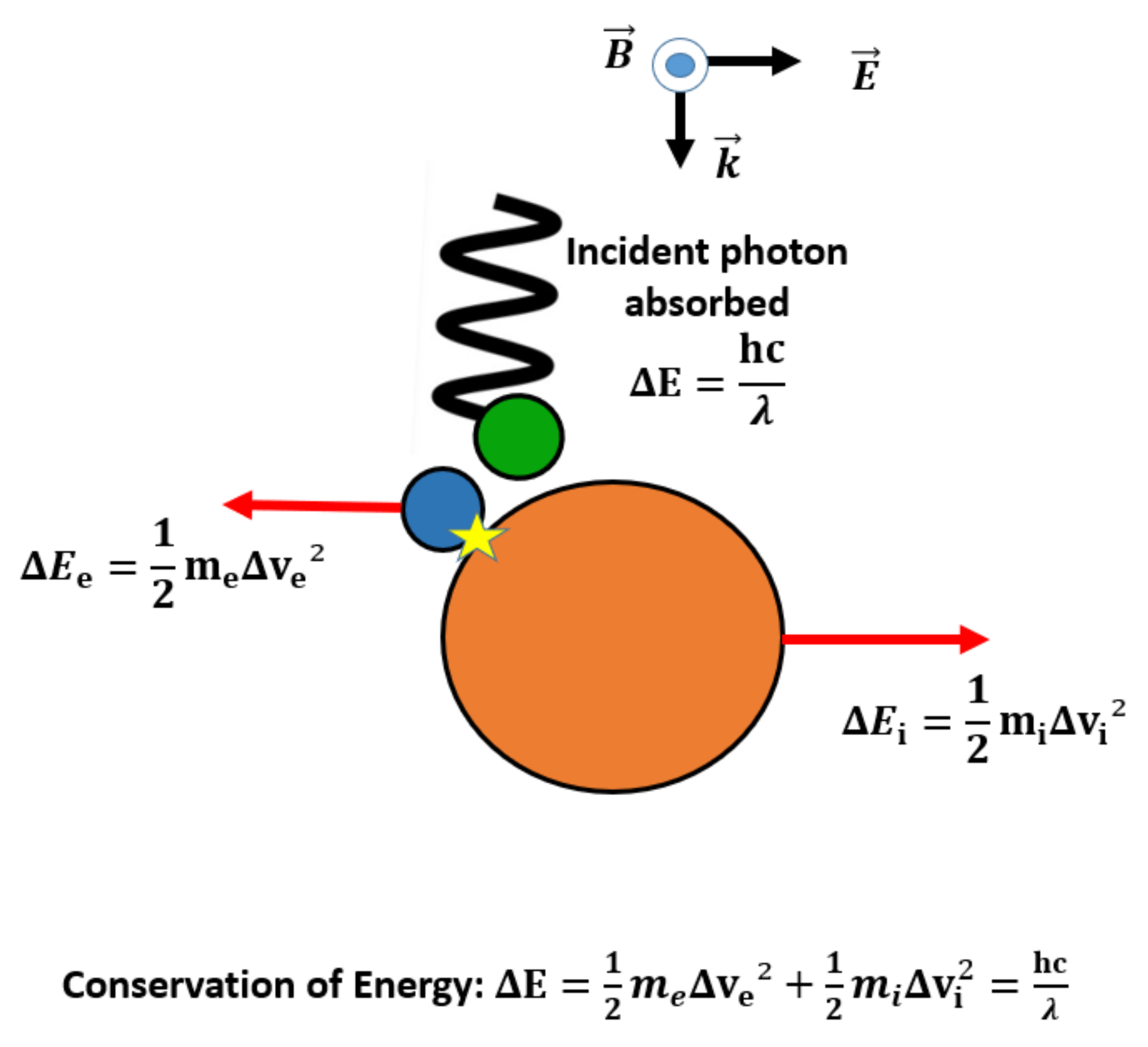
• In a second step, the absorption of the laser energy by the plasma is assumed to be close to 100%. The main mechanism of absorption involved here is the inverse Bremsstrahlung (IB [42], as can be seen in Figure 3). IB is a collisional process involving three particles: a photon, an electron, and an ion. By conservation of the momentum, the photon’s energy is absorbed and the kinetic energy of both the ion and the electron are increased. Furthermore, electrons are accelerated in the electrical field of the laser and they transfer their energy to heavy particles by collision, leading to a global increase in plasma temperature.
  Thus, this mechanism is highly dependent on the frequency ${\nu }_{ei}$ at which the electron and ion collide.
  This frequency may be obtained using Lorenz’s model [43,44]:

  $${\nu }_{ei}\propto \frac{n_e{Z}_i}{T^{\frac{3}{2}}}$$

  (7)

  where $n_e$ is the plasma electronic density, $Z_i$ is the ionization state, and T is the temperature.
  Altogether, the optical index of the plasma is given by

  $$n=\sqrt{{ϵ}_p}$$

  (8)

  where ${ϵ}_p$ is the permittivity of the plasma:

  $${ϵ}_p\approx 1-\frac{n_e}{n_c}-i\frac{n_e{\nu }_{ei}}{n_c\omega }$$

  (9)

  where $n_c$ (in cm ${}^{-3}$, with $\lambda$ in nm: $n_c\approx {10}^{27}{\lambda }^{-2}$) is the critical density of the plasma:

  $$n_c=\frac{m_e{ϵ}_0{\omega }^2}{e^2}$$

  (10)
  As the absorption coefficient ${\alpha }_{IB}$ is related to the imaginary part $n_2$ of the refractive index:

  $${\alpha }_{IB}=\frac{2n_2\omega }{c}$$

  (11)
  Thus, the absorption by IB is given by

  $${\alpha }_{IB}\propto \frac{n_e^2{Z}_i{\lambda }^2}{T^{\frac{3}{2}}}$$

  (12)

  where $\lambda$ is the laser wavelength.
  Finally, if we consider a linear variation of the electronic density from 0 (at the plasma outside surface) to $n_c$ (in the depth of the plasma) on a total length L, then we have:

  $$A_{IB}\propto 1-{\mathrm{e}}^{-\frac{Z_{i}L}{{\lambda }^2{T}^{\frac{3}{2}}}}$$

  (13)
  Hence, the absorption $A_{IB}$ by IB on this length L of the plasma appears to be more effective at a shorter wavelength. This observation is confirmed by experimental results that show that the pressure was higher at shorter wavelengths, whilst all other parameters remain the same [26,45].
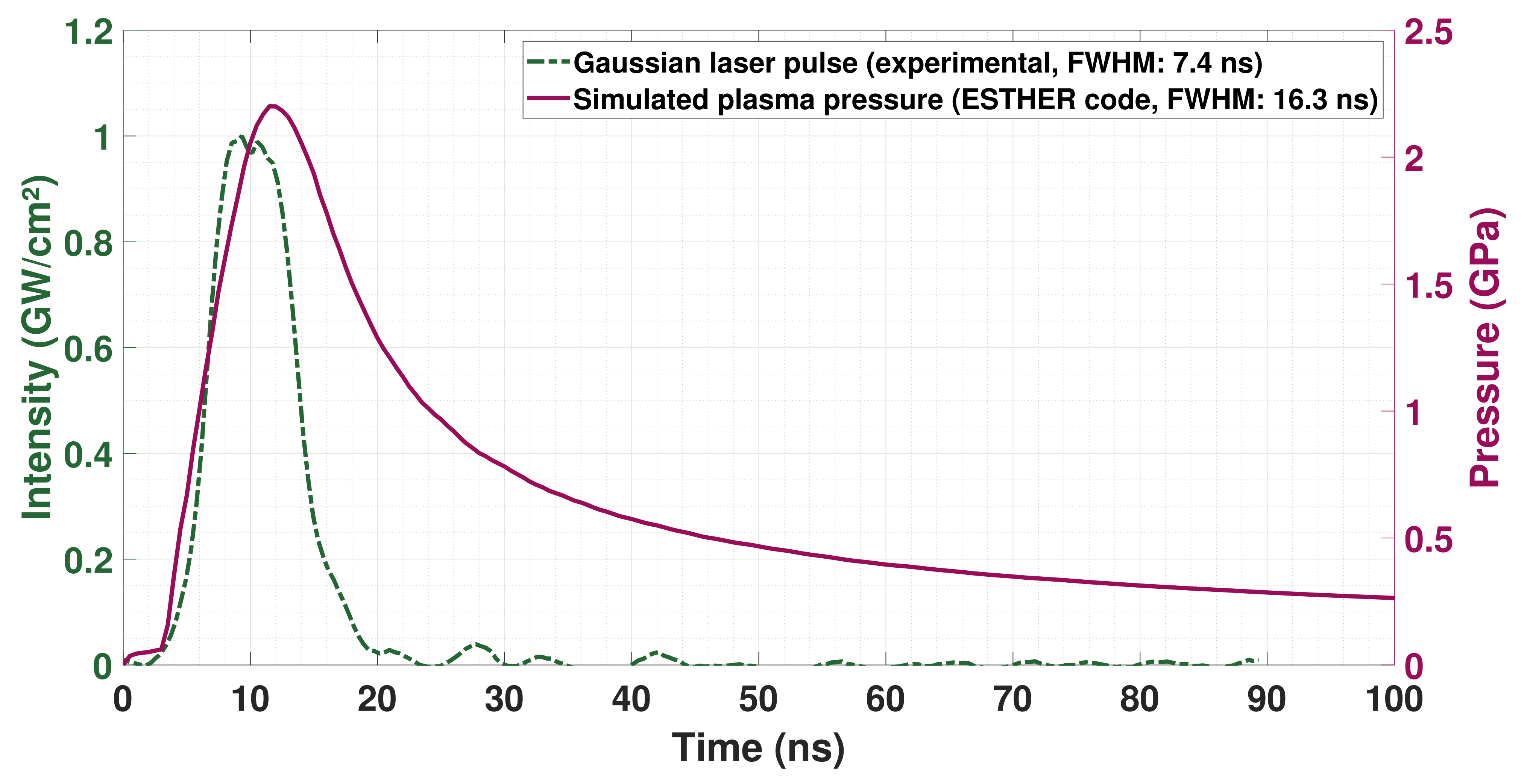
• The last step begins at the end of the laser pulse ($t_e\approx 2\tau$, $\tau$ the laser pulse duration (FWHM)). The pressure of the plasma starts to decrease following an adiabatic law of Laplace:

  $$P\left(t\right)V{\left(t\right)}^{\gamma }=P\left(t_e\right)V{\left(t_e\right)}^{\gamma }$$

  (14)
  The pressure maintained in this last part is no longer useful for the shock process. However, the temperature is greatly important as the duration of this slow adiabatic release will mainly drive the thermally affected depth and thus whether the thermal protective coating shall be used.
  Indeed, a 1D thermal model (temperature $T_{1D}$ applied during a duration ${\tau }_{1D}$) gives the following depth that will be affected by the heating:

  $$z_{1D}=\sqrt{{\kappa }_m{\tau }_{1D}}$$

  (15)

  where ${\kappa }_m$ is the thermal diffusivity; typical values for $z_{1D}$ range within a few micrometers in laser shock processes.
  To reduce the thermally affected depth $z_{1D}$, one should ensure that the duration ${\tau }_{1D}$ of the plasma’s thermal loading is as short as possible.
  Furthermore, depending on the used laser spot size, a rarefaction wave propagates from the edges of the plasma towards its center. When it arrives at the center ($t={\tau }_R$), a fast release of the pressure occurs which has been previously described by Pirri [46,47]:

  $$P\left(t\right)\propto {\left(\frac{t}{{\tau }_R}\right)}^{-\frac{6}{5}}$$

  (16)

2.2.2. Breakdown Plasma Generation

When very high intensities are reached, the dielectric confining medium (water, quartz, ...) stops being transparent to the incident laser pulse. Indeed, a breakdown plasma is created and thus the laser pulse is absorbed in that plasma instead of being absorbed by the plasma on the metal target. As a consequence, the laser intensity that may reach the target starts saturating at a value $I_b$ which is the breakdown intensity threshold of the confinement.

Previous works have studied these breakdown plasmas, and tried to numerically simulate them [48,49].

There are two mechanisms involved in the breakdown generation in dielectric medium:

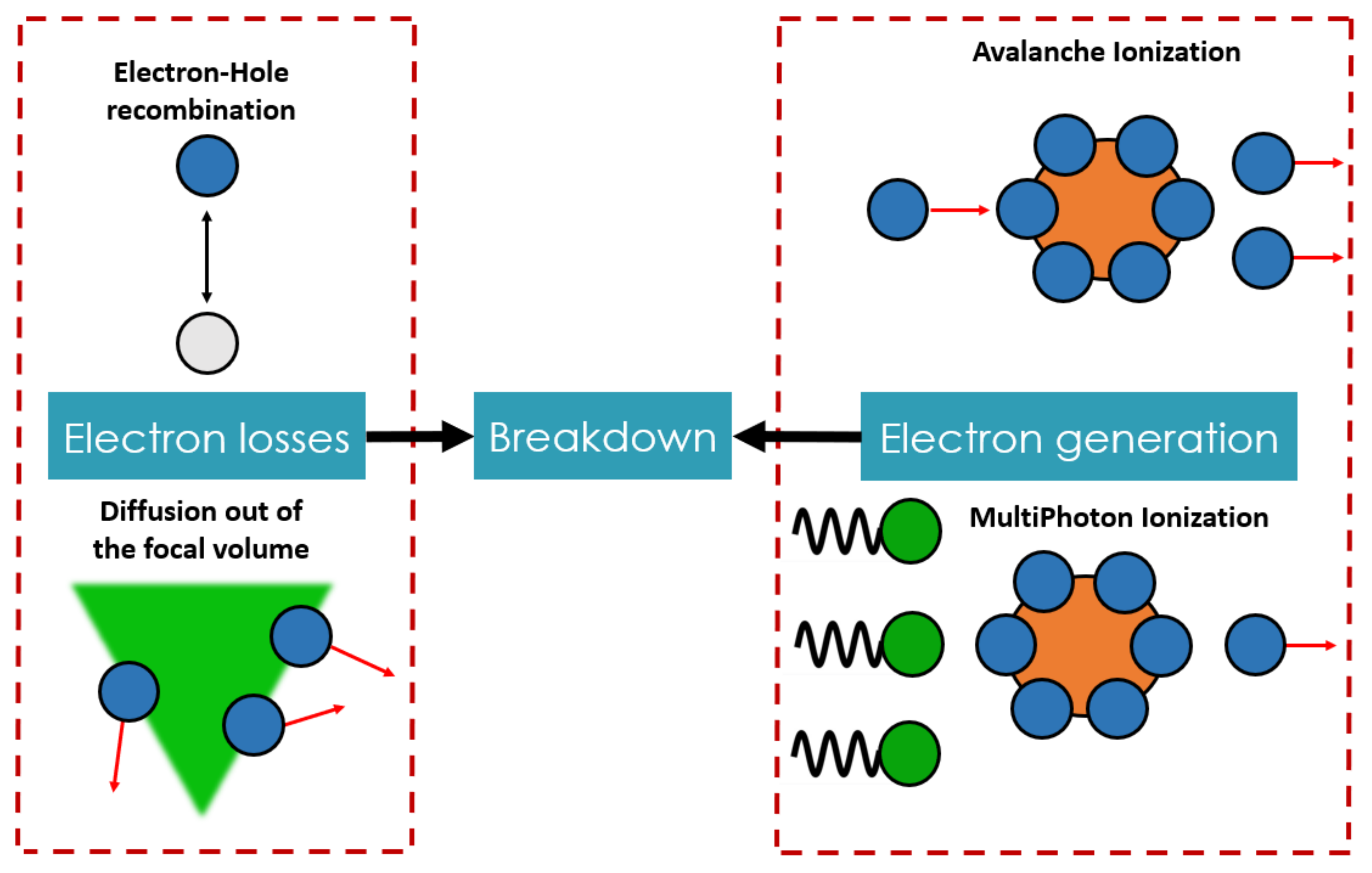
• Avalanche ionization (AI)—here, electrons are accelerated by the electrical field of the laser pulse: their kinetic energy ($E_{k,e}$) increases and becomes sufficient to ionize an atom ($E_{k,e}>\Delta E_e$, with $\Delta E_e$ being the ionization potential). This mechanism evolves exponentially: for one initial electron, and after n avalanche processes, there will be $2^n$ electrons created.
  If ${\eta }_{AI}$ is the rate of AI per electron, then the density evolution is given by

  $${\left[\frac{\mathrm{d}{n}_e}{\mathrm{d}t}\right]}_{AI}={\eta }_{AI}{n}_e$$

  (17)
  The rate of AI, ${\eta }_{AI}$, was calculated by Kennedy [50]. To be effective, this mechanism requires either a minimal number of electrons (seeds) to generate the breakdown or longer laser pulse duration. In the case of water confinement, the initial density has been estimated to be approximately ${10}^9$ cm ${}^{-3}$ [48].
• MultiPhotonIonization (MPI)—k (k an integer) photons are simultaneously absorbed by the atom (ionization) if the following condition is obtained:

  $$\frac{khc}{\lambda }\ge \Delta E_e$$

  (18)

  where h is the Planck constant, c is the speed of light, $\lambda$ is the wavelength and $\Delta E_e$ is the ionization potential of the atom.
  As this is a quantum process, it can be shown that this mechanism is less effective with a higher value of k (thus a higher value of wavelength $\lambda$).
  Keldish and Morgan have given values and models to calculate the electron generation by MPI [51,52].

From these two mechanisms of electron generation, one should add the following losses:

• The electrons leaving out the focal volume by diffusion. If we use a rate ${\eta }_d$ of diffusion per electrons, the variation on the density is given by

  $${\left[\frac{\mathrm{d}{n}_e}{\mathrm{d}t}\right]}_d=-{\eta }_d{n}_e$$

  (19)
• Losses by recombination: an electron–hole pair is recombined at a rate of ${\eta }_r$ per electron and hole. Then, the density variation is given by

  $${\left[\frac{\mathrm{d}{n}_e}{\mathrm{d}t}\right]}_r=-{\eta }_r{n}_e^2$$

  (20)

Hence, an equation of rate combining all of these mechanisms (summarized in Figure 4) may be used:

$$\frac{\mathrm{d}{n}_e}{\mathrm{d}t}={\left[\frac{\mathrm{d}{n}_e}{\mathrm{d}t}\right]}_{AI}+{\left[\frac{\mathrm{d}{n}_e}{\mathrm{d}t}\right]}_{MPI}-{\left[\frac{\mathrm{d}{n}_e}{\mathrm{d}t}\right]}_d-{\left[\frac{\mathrm{d}{n}_e}{\mathrm{d}t}\right]}_r$$

(21)

Finally, by solving Equation (21), one can obtain the evolution of the electron density in the confinement medium. The breakdown is assumed to be effective when the electron density $n_e$ reaches the critical density ($n_c$, Equation (10)): from this value, the laser can no longer pass through this breakdown plasma.

The breakdown can be experimentally measured by three main ways:

• A direct observation through an intensified camera—this experiment was conducted by Berthe et al. and it shows that the breakdown plasma appears at the surface of the confinement layer [22,25].
• By measuring either the pulse duration or the transmission (in energy) of the laser pulse through the confinement—as soon as the breakdown starts, the transmitted pulse duration (or the transmission in energy) starts to decrease with the increase in laser intensity [22,23,24].
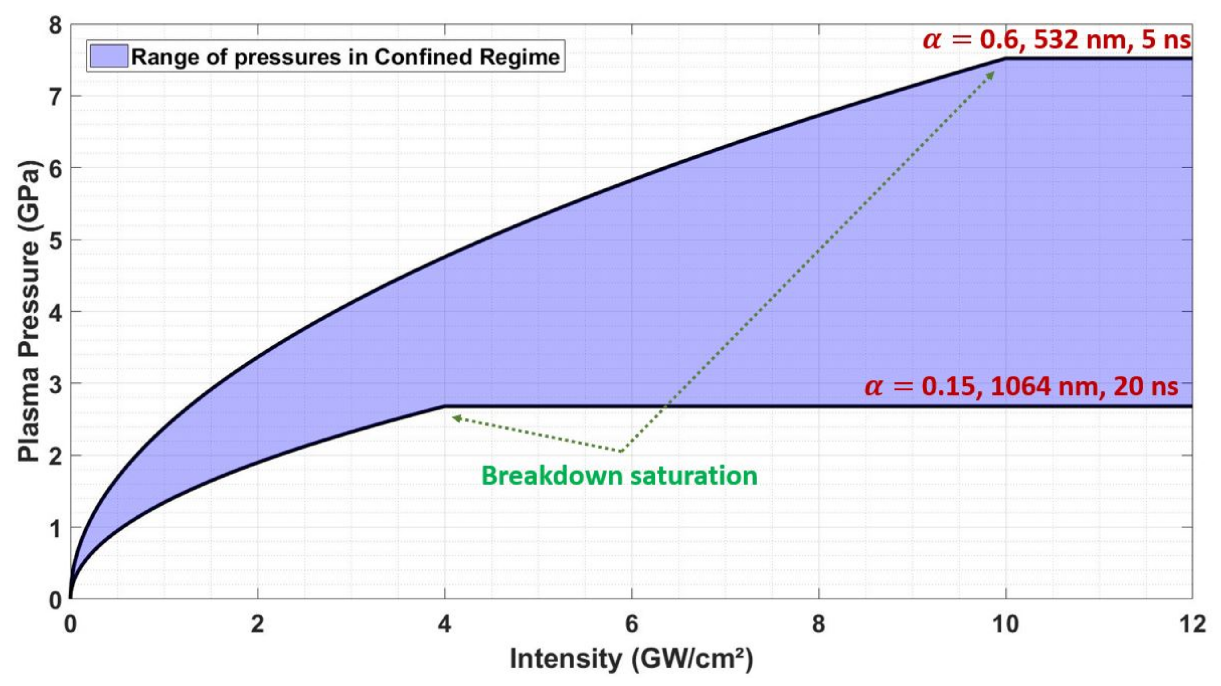
• By measuring the pressure of the plasma (see the following part concerning the rear-free surface indirect determination of the plasma pressure)—when the breakdown threshold is reached, the pressure stops increasing with the laser intensity and fluctuates around a maximum value associated with the pressure value at the breakdown intensity threshold $I_b$ [23,25,26,27].

Values for the breakdown threshold in water were experimentally measured at three different wavelengths for a pulse duration (FWHM) $\tau$ = 25 ns. Thresholds were found to be $I_{b,\omega }$ = 10 GW/cm²; $I_{b,2\omega }$ = 6 GW/cm²; $I_{b,3\omega }$ = 4 GW/cm² at 1064 nm, 532 nm and 355 nm, respectively, [26]. More recent experiments performed at 1064 nm and 532 nm, for a pulse duration of 7 ns, gave different results: $I_{b,\omega }$ = 8 GW/cm² and $I_{b,2\omega }$ = 10 GW/cm² [53].

The obtained tendency regarding the wavelength dependency and the threshold values are quite different between previous measurements (approximately 25 ns) and current ones (approximately 7 ns). This may first be explained by the fact that AI and MPI do not have the same importance as functions of pulse duration in the ionization mechanism. Furthermore, a lot of improvements have been made in recent years regarding optical metrology.

The maximum pressure $P_m$ reached at the breakdown was also obtained: $P_{m,\omega }$ = 6 GPa; $P_{m,2\omega }$ = 6 GPa; and $P_{m,3\omega }$ = 4 GPa.

Berthe et al. concluded that at a shorter wavelength, even if the absorption by the plasma by IB is better, the breakdown phenomenon starts sooner as the MPI phenomenon is more effective [26].

More recently, breakdown phenomena were investigated in a water tank configuration (WTC) [54]. Based on unprecedented experimental results (direct measurements of the transmitted energy and of the laser pulse duration through the water confinement; indirect measurements of plasma pressure and sample surface sinking after LSP treatments), it has been demonstrated that the breakdown threshold (for a 7 ns FWHM laser pulse at 532 nm) is increased from 10 GW/cm² (when it occurs at the confinement surface as it classically does) to more than 20 GW/cm² when it occurs at a depth (volume) of water confinement. Hence, the purpose of the WTC is to use a high thickness of confinement to ensure that the laser intensity at the confinement surface is weaker than the known breakdown threshold; thus, the breakdown will only occur in a volume of the confinement, at a higher threshold (at least two times higher). Finally, the maximum pressure of saturation will be increased to 10–12 GPa instead of 6–8 GPa (when a small layer configuration is used).

These results may help address new applications as higher pressures are reached. Furthermore, they may also impose the use of a green visible wavelength (532 nm) for LSAs.

Even though the mechanisms involved here to explain this different behavior regarding whether the breakdown is created in depth or at the surface of the confinement are not yet understood, it should change the habits of the LSP community concerning the use of LSP under water. Further research works should focus on the physics behind breakdown plasmas in dielectric medium to improve our general understanding.

2.3. Experimental Data and Characterization of Confined Plasmas

Until recently, most experimental studies concerning laser interaction in a confined regime have been focused on investigating the dynamics of induced shock waves and exploring the conditions which optimize the shock pressure imparted to the sample. Indeed, the amplitude and duration of these shock waves are the main processing parameters for most laser shock processing applications [12,55,56,57,58], which to date have been the primary users of confined laser-matter interaction.

However, in recent decades, new fields of research using confined laser-matter interaction have emerged such as the laser synthesis of colloidal nanoparticles (LSC) [59,60] and laser-induced breakdown spectroscopy (LIBS) for surface elemental analysis [61]. For these applications, a good knowledge of the confined plasma parameters is critical, because they strongly impact their effectiveness. Therefore, in recent years, various experiments were performed in order to characterize the properties of the plasmas generated by the pulsed laser irradiation of solid–liquid interfaces.

Kanitz et al. recently published a very complete review summarizing most of these studies [39]. Several experiments have shown that the ablation rate in water confinement is higher than in air, and this increased ablation efficiency is attributed to the higher plasma pressure as a consequence of the confinement [62]. Indeed, the observations performed with intensified charge-coupled devices (ICCD) show that the plasmas generated in liquids are confined closer to the test piece than the ablation plasma in gaseous media, which further expands into the gaseous environment immediately after the laser pulse [10,62,63,64,65,66]. The light emission region has an elliptical shape above the surface and its size is roughly one-tenth of the maximum size obtained in air [63].

Nguyen et al. [62] have shown that for the same laser pulse intensity, the plasma expansion during and after the laser pulse follow different mechanisms: the plasma plume that grows in the air follows a radiation-wave model (LSR) [67] while a detonation-wave model (LSD) [68] can explain the expansion of the plasma plume induced in water. This is consistent with the observations of Sano et al. [10] which show that the plasma expansion velocity in water is equal to sonic velocity. Furthermore, the 1D hypothesis on the plasma expansion is shown to be not valid for the used spot size (0.75 mm). As a consequence of the high confinement effect and the higher ablation rate, the atomic densities in the confined plasma are very high.

By measuring the size of the plasma-emitting region and the ablation rate, Saito et al. [63] roughly estimated an atomic density of 6.7 × 10${}^{21}$ cm ${}^{-3}$, whereas Takada et al. [65] found values ranging from 1 ×${10}^{20}$ to 1 ×${10}^{21}$ cm ${}^{-3}$. From the Saha equation, Dell’Aglio et al. [66] calculated atomic densities from 3 × 10${}^{19}$ to 1 ×${10}^{20}$ cm ${}^{-3}$.

In order to determine the plasma parameters such as plasma temperature and electron density, emission spectroscopy (either atomic or molecular) measurements were carried out by various investigators.

Sakka and their coworkers were the pioneers of such studies in the early 2000s [38,63,64,69,70,71,72,73,74,75,76,77]. In particular, they have shown that emission intensity and emission profile strongly depend on the laser pulse duration [64,73,75,76,77]. However, the investigated intensities were quite low (0.5 GW/cm²) compared to those used in LSP. The images of the plasma-emitting region generated by 20 ns laser pulses display several spots with bright centers and the resulting spectra are broad and continuous. Indeed, as a consequence of the white light emission from these high-density bright spots, the emission spectra obtained with short laser pulses suffer from broadening and self-absorption. With laser pulses longer than 40 ns (typically 150 ns in their studies), the size of the light emitting region increases and the bright spots disappear. Emission is more homogeneously distributed with the brightest region at the center of the hemispherical ablation plume. In this case, one obtains spectra with clear narrow emission lines at longer delays, because excitation by the later part of a longer pulse expands the plume and reduces its density, therefore reducing the broadening of the emission lines and the self-absorption inside the plasma.

Different groups have tried to extract the density from emission spectra, either using the Stark broadening of the neutral emission line or fitting the continuum emission decay induced by electron–ion recombination [66,69,78,79,80,81,82]. For laser pulse durations of 5 to 10 ns, the measured electron densities range from 5 × 10${}^{17}$ to 1 × 10${}^{20}$ cm ${}^{-3}$, with a general decay in time after the laser pulse (see Figure 8a of reference [39]). These values are up to one order of magnitude higher than those recorded in air [80,82]. Similarly to the electron densities, the temperatures of different species were extracted from optical emission spectra using different methods:

• Fitting of a Planck-like distribution to the continuous background (this usually requires a plasma in thermodynamic equilibrium emitting a type of black body radiation);
• Excitation temperature obtained by comparing the relative intensities of the emission lines of an atomic system;
• Rotational and vibrational temperatures obtained by fitting the rovibrational spectrum of a well-defined electronic transition.

The temperatures measured by the different groups, which are summarized in Figure 8b of reference [39], range from 2000 to 8000 K. Among all these measurements, the excitation temperatures are the highest with values of approximately 8000 K at the beginning of the plasma, and then decaying within hundreds of nanoseconds up to approximately 4000 K [81,82]. The Planck temperatures are a little bit lower, ranging from 7000 K down to 4000 K, equally with the measurements of the vibrational temperatures [70,71,78,83,84]. The measured rotational temperatures seem to be lower than the measured vibrational temperatures [70,71,78,85], which indicates that the temperatures of different species within the plasma are not in equilibrium at long delays. All these measurements display fast cooling during the first 200 ns which is a direct consequence of the strong interaction of the plasma with the cold liquid environment [85,86,87,88]. This last point highlights the necessity to take into account the contribution of the confining medium when one wants to simulate the behavior of the confined plasma.

As most of these measurements were conducted at low intensities (<1 GW/cm²), there is still a strong need to investigate higher intensities (up to 10 GW/cm²).

2.4. Development of Diagnostic Systems for Pressure Measurements

As it is the most experimentally accessible datum and the one directly linked with the process, the plasma pressure is probably the most important source term on which to focus on. Indeed, this pressure source term is of a great importance for simulations of LSP, as this will be used as an input to simulate the propagation of shock waves inside the treated sample. Furthermore, from the shock waves propagation, the induced residual stress field at a depth of the treated material can also be calculated, and hence the fatigue behavior of the component may be obtained. This is also an information which is not burdensome to obtain nor difficult to experimentally implement, as many diagnostics exist, based on the measurement of a shock wave. However, one should keep in mind that this pressure measurement is always an indirect measurement: some considerations about used devices, material parameters, and shock waves propagation must be used to get back to the plasma pressure, always deduced from the induced shock-wave velocity at the rear-free surface of the irradiated samples.

In each situation, the rear pressure is either measured from the rear surface material velocity (use of a BK7 glass plate for example, to prevent the back-and-forth of the shock wave) or either from the rear-free surface velocity (being twice of the material velocity), as illustrated in Figure 5. Mainly three parts may be identified: the elastic precursor; the shock wave, that stiffens up as the pressure increases; and the release wave, which spreads out as the pressure decreases. The peak velocity is associated with the peak pressure. Indeed, knowing the thickness of the sample and its attenuation, the plasma peak pressure at the top of the sample is determined.

Using the equation of the conservation of momentum, the pressure is given by

$$P_{\mathrm{plasma}}=\rho (C_0+Su)u+\frac{2{\sigma }_{y_0}}{3}+\delta P$$

(22)

where u is the (experimentally measured) material velocity, $\rho$ is the density of the metal target, $C_0$ is the bulk sound velocity, and S is the Hugoniot constant (material depending; S = 1.38 for aluminum alloys). $\delta P$ is the attenuation of the shock wave during its propagation from the top to the rear surface, and $\frac{2{\sigma }_{y_0}}{3}$ is the elastic contribution (${\sigma }_{y_0}$ being the elastic limit).

However, Equation (22) only provides the plasma peak pressure, and numerical simulations are required (with software such as Abaqus) to obtain the full plasma pressure temporal profile, which is the one that reproduces experimental signals (Figure 5).

In this part, various systems to measure the plasma pressure will be presented with their associated advantages and drawbacks. In the end, a methodology will be given to explain how to properly and easily measure the used plasma pressure.

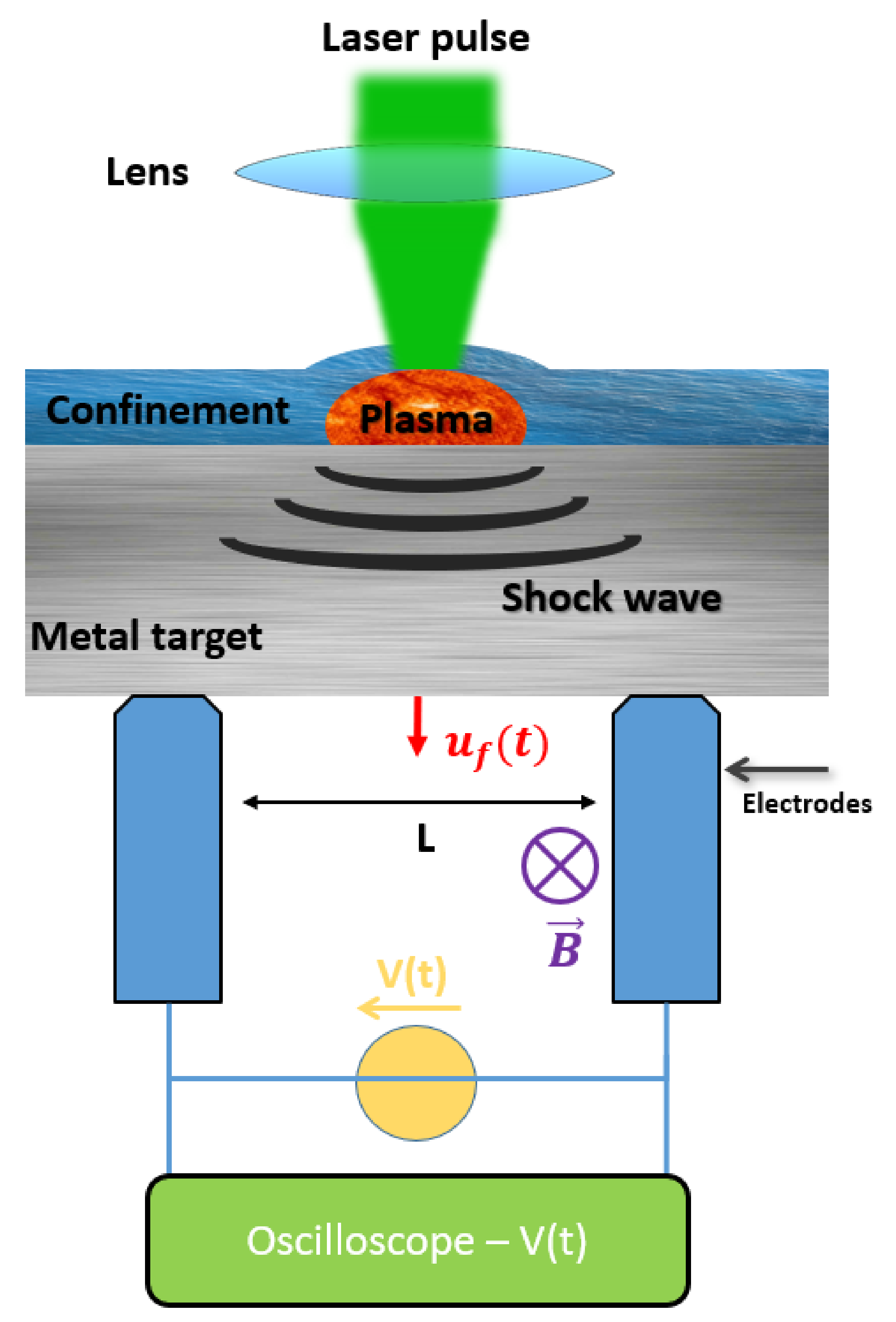
• Electromagnetic Gauge
  This method uses the displacement of the metal induced by the shock wave when it arrives at the rear surface of the target [89,90,91].
  As shown in Figure 6, the target is placed in a constant magnetic field B (created by two magnets for example), and two metallic pins are connected to the target and separated by a distance L. Following Faraday’s law of induction, when the shock wave arrives at the rear surface and makes it accelerate, the created displacement $u_f$ in the magnetic field will induce a voltage $V_U=u_{f}BL$, which corresponds to the variation in magnetic flux ($\frac{d{\Phi }_B}{dt}=-V_U$) through the wire loop.
  As, in this case, the rear surface is free, the measured rear free velocity $u_f$ is twice the material velocity u (reflection of the shock wave at the metal/air interface). Equation (22) then gives:

  $$P_{\mathrm{plasma}}=\frac{\rho (C_0+S\frac{V_U}{2BL})V_U}{2BL}+\frac{2{\sigma }_{y_0}}{3}+\delta P$$

  (23)
  This method has some advantages: it is an easy experimental setup to implement, and signals are directly related to the velocity without complicated treatments to be applied. Furthermore, a good temporal resolution is obtained, which is given by the speed of used oscilloscopes (typical resolution will be 0.3 ns with a 10 GS/s oscilloscope with a bandwidth of 2 GHz).
  However, there are a lot of possible uncertainties:

  −

  The magnetic field may vary during the process, mainly because of the perturbations induced by the plasma;

  −

  The distance between the two electrodes, which is constrained by the size of the laser spot size (a few mm) may also vary and be inaccurately measured. It may also be difficult to ensure that both electrodes are in contact with the target;

  −

  Typical values used for B (0.2 T) and L (1 mm) will give low voltage (40 mV for a maximum rear velocity of 200 m/s) and the signals may thus be noisy.

• PVDF Piezoelectric System
  A piezoelectric material, for which PVDF (polyvinylidene fluoride) is often chose, in laser shock experiments [91,92,93], is bonded on the rear-surface of the metal target. When the shock wave arrives at the interface between the metal and the PVDF, a part of the shock wave is transmitted and starts to propagate in the PVDF. As a result, it will undergo elastic deformation, and by a piezoelectric mechanism, a current will be generated. By measuring the electrical current generated between the front and back face of the PVDF, one can deduce the pressure of the shock wave. Thus, by taking into account the mismatch impedance between the metal and the piezoelectric material, the shock wave pressure at the rear surface of the metal can be deduced. Altogether, similarly to the previous measurement of the rear-surface by electromagnetic gauge, the pressure of the plasma is indirectly calculated.
  When the shock arrives at the interface, moving at a material velocity u, the intensity $I_c$ is given by: $I_c{e}_0=P_{0}u$ where $e_0$ is the thickness of the piezoelectric system and $P_0$ is the ferroelectric polarization.
  Though this system is quite easy to use and implement, there are a lot of drawbacks:

  −

  The material parameters of the piezoelectric medium must be precisely known, which is not often the case (calibration of $P_0$);

  −

  At high pressure (>5 GPa), the material starts to respond non-linearly, making the pressure measurement inaccurate;

  −

  Some calculations have to be made to estimate the mismatch impedance in order to obtain the pressure at the rear surface of the metal target;

  −

  As with gauges, the electrical signal may be disturbed by the electromagnetic field of the plasma, especially at high laser intensity;

• PDV
  Photonic doppler velocimetry (PDV) is based on the concept of heterodyning, but it has only recently been developed as a useful shock-physics diagnostic, thanks to the recent technological advances of the telecommunications industry [94,95]. In its simplest configuration (a light and compact system, with full optical beam transportation through fiber), PDV is a fiber-based Michelson interferometer in which laser light is divided among two paths: the first one containing the target and the other one a stationary reference mirror. The laser Doppler-shifted light coming back from the moving target is combined with the reference light and sent to an optical receiver. The optical interferences which are generated result in a beat frequency $f=\frac{2}{{\lambda }_0}|vs.|$, where ${\lambda }_0$ is the wavelength of the laser probe. At 1550 nm, which is the typical wavelength of most PDV systems, every km/s of velocity v requires 1.29 GHz of receiver/digitizer bandwidth. The velocity is finally extracted from the recorded signal through a time–frequency analysis, typically performed with short-time Fourier transforms (STFTs) [96]. The main advantages of PDV are its ease of use, its robustness, and its relatively low cost compared to other diagnostics such as VISAR. Moreover, because PDV tracks motion in a frequency-encoded temporal electro-optical signal, it is thus able to record multiple velocities simultaneously. However, like all other diagnostics, PDV also has some drawbacks:

  −

  The primary weakness of conventional PDV is its inability to resolve low-velocity transients;

  −

  Conventional PDV measurements are also directionally blind: motion toward and away from the probe lead to the same beat frequency;

  −

  Due to the use of time–frequency analysis to retrieve the velocity, the velocity resolution is inversely proportional to the time resolution. Thus, considering the fact that plasma-induced shock waves involve a short duration (in the nanosecond range), with a required resolution of approximately 1 ns, the resolution on velocities is then limited to approximately 50 m/s.

  Because of its novelty, PDV has only been scarcely used for laser shock characterization [97,98,99], and to the authors’ knowledge, only one recent work has been performed in the frame of LSP using PDV [100].
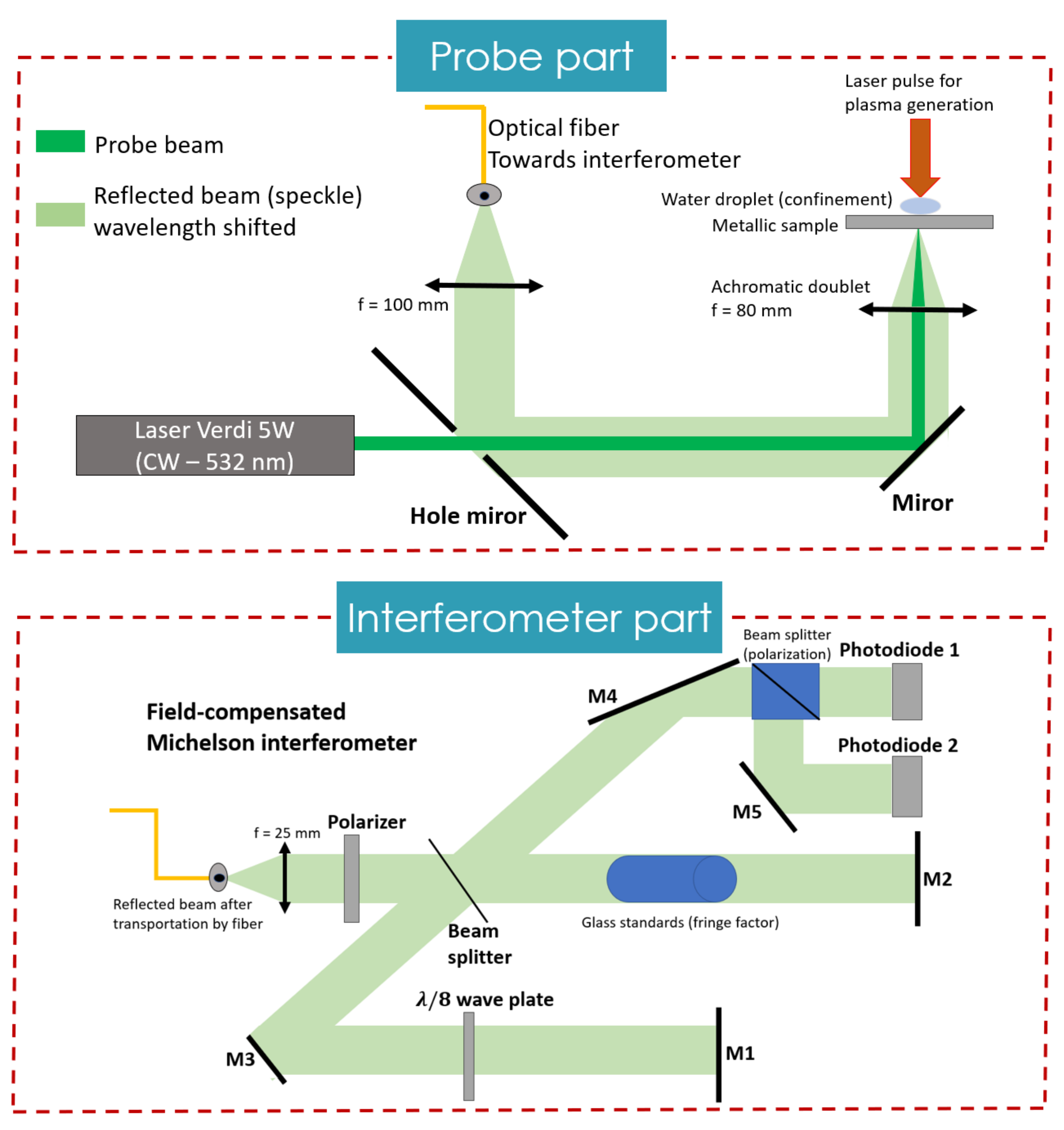
• VISAR Optical System
  The Velocity Interferometer System for Any Reflector (VISAR), developed by Barker in 1972 [101]), is currently the most used system to measure plasma pressure: it also aims to measure the rear-free surface velocity of the target. An accurate optical measurement was performed.
  As shown in Figure 7, the VISAR is made of two parts (the probe part and the interferometer part):

  −

  The probe part—a single longitudinal mode (${\lambda }_0$ with a narrow spectral width) collimated laser beam is focused on the rear surface of the metal target. The scattered reflection of the beam is then collected (using a short focal length) and directed towards the second part to be analyzed. This reflection is wavelength-shifted according to the Doppler–Fizeau effect as the surface is moving under a free velocity $u_f$ ($\lambda \left(t\right)={\lambda }_0(1-\frac{2u_f\left(t\right)}{c})$).

  It may be preferable to use an unpolished sample to generate more scattered light compared to the specular reflection that could be deflected out of the interferometer if the sample is becoming excessively deformed (which often occurs for thin samples of ≈100 µm).

  −

  The interferometer part—this second part is a field-compensated Michelson-like interferometer. Calibrated glass enables to delay one arm of the interferometer from the other. This changes the initial path difference (${\delta }_i$) in the interferometer, and hence the required velocity to move from one fringe to the next one is also changed: this is the velocity per fringe (VPF) factor. Then, the interference between the signal at a time t (wavelength $\lambda \left(t\right)$) and one at a time $t+\Delta t$ (wavelength $\lambda (t+\Delta t)$) is produced, and the interferogram’s intensity is acquired with a fast PhotoMultiplier (PM). Therefore, there is a translation of the interference fringes as soon as a wavelength-shift occurs. The time resolved measurement of the interference intensity enables one to obtain the corresponding velocity.

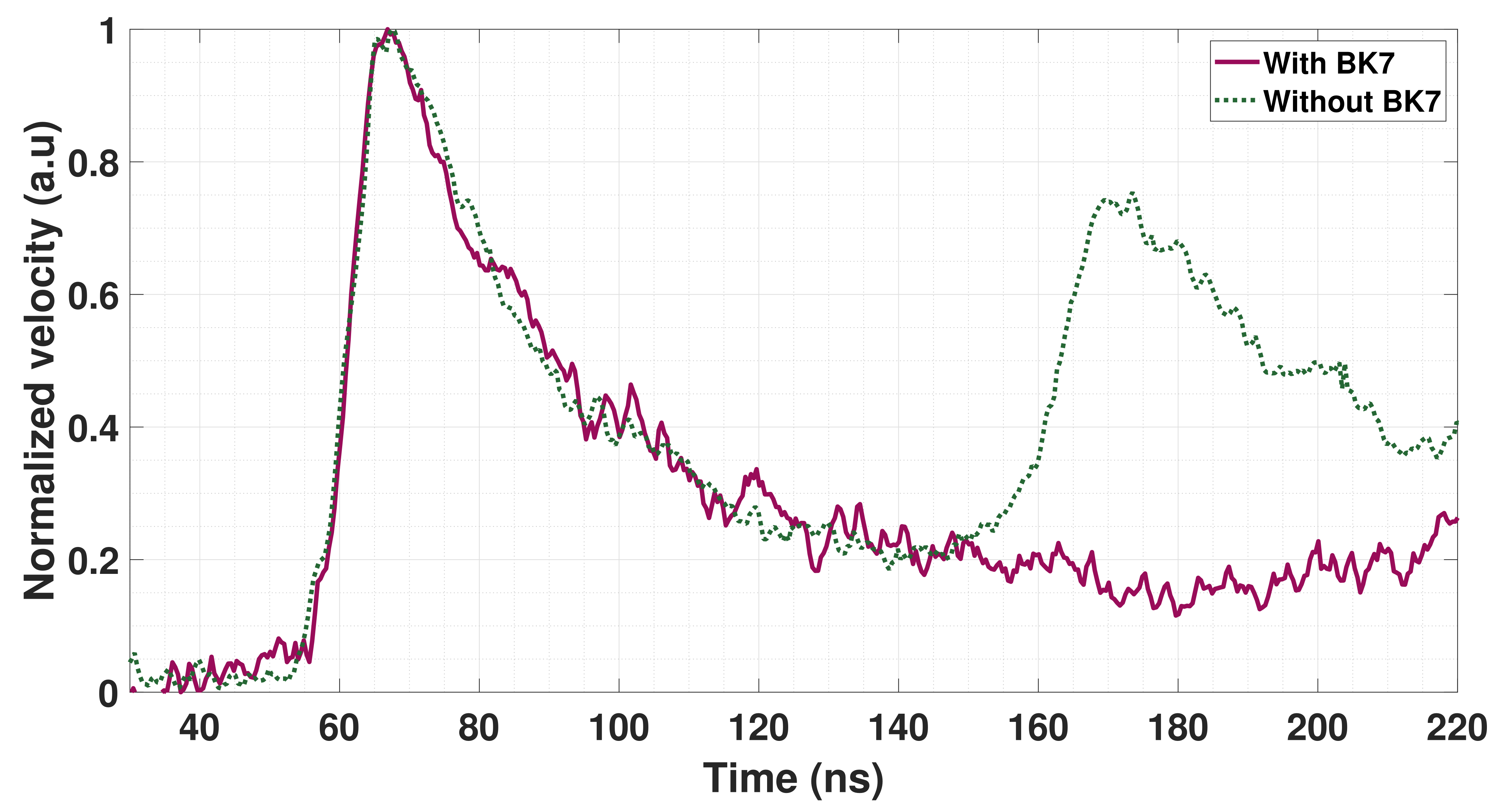
  The intensity of the interferogram follows the following law: $I_v\left(t\right)\propto 1+cos(\frac{2\pi {\delta }_{i}c}{{\lambda }_0(1-2u_f\left(t\right))})$. Consequently, a simple code has to be used to analyze the intensity signals obtained on the PM in order to obtain the rear-free surface velocity $u_f$. Thus, as for EM gauge, the plasma pressure is given by

  $$P_{plasma}=\frac{\rho (C_0+S\frac{u_f}{2})u_f}{2}+\frac{2{\sigma }_{y_0}}{3}+\delta P$$

  (24)
  The VISAR system is the most resilient and reliable means of plasma pressure measurement: it is without contact (and therefore not influenced by the process) and it can even be used at very high pressure. However, it is not the easiest system to implement as it must be carefully aligned. Indeed, both the probe laser beam (to be brought under the target) as well as the interferometer system (to analyse the wavelength shift) must be properly adjusted. Furthermore, a wise choice of calibrated glass length has to be made before the measurement beings, and some calculations must be performed to obtain the rear-free surface velocity.
  Finally, a great temporal resolution of less than 1 ns is achieved, only limited by the PM response-time. For all these reasons, we recommend using this system for pressure measurements as it offers the best compromise between assets and drawbacks.
• Method to Measure the Plasma Pressure with VISAR
  It is important to measure the plasma pressure as accurately as possible as a function of the used laser parameters. Indeed, this will help perform simulations but also to use specific though not very well known material such as FSW materials which possess specific properties [102]. If one knows precisely, for a given laser configuration, the loading pressure term of the plasma, then it helps to more effectively extract the material parameters from a typical shock-wave measurement, as previously shown.
  First of all, we recommend using a well-known material, such as pure aluminum with a small thickness, to perform laser-induced shock-wave measurements. This will help prevent the dependency of the results with the material parameters or models.
  Secondly, we suggest using large laser spot sizes to prevent the interferences of complex phenomena such as edge effects (also called 2D effects) [103,104]. Keeping the shock wave as monodimensional as possible should be ensured whenever possible.
  Moreover, regarding VISAR optical measurements, one should use an unpolished target in order to avoid a loss of the optical signal.
  On the other hand, in the case of very thin samples which may become deformed under the shock (thus making the pressure measurement difficult to conduct), we recommend sticking a transparent glass window to the rear surface of the sample, such as a BK7 glass plate for aluminum (as performed in [37]). This window must have a mechanical impedance as close as possible to the target on which it will be stuck. Under these conditions, the shock wave is transmitted between the sample and the window without reflection and the full profile of the shock wave can be measured (as shown in Figure 5). One should note that in this case, the material velocity is measured and is half the value of the free surface velocity.

3. Improvements in Experimental Accuracy—Range of Plasma Pressure Data Obtained

3.1. Improvements in Optical Metrology and Better Understanding of Materials Behavior

Nowadays, the energies and pulse durations of laser are quite precisely obtained: the uncertainty in the pulse duration is approximately 0.1 ns in the 10 ns range ($\Delta \tau$/$\tau$ being equal to 1%) while the uncertainty in the energy is approximately 10 mJ in the J range (with $\Delta E$/E being equal to 1%). Furthermore, significant improvements were made in laser design, leading to more stable and reproducible systems. Common values of stability are often given as less than $0.5\%$ for the energy and less than $5\%$ for the pulse duration (RMS).

On the other hand, the laser spot size was also more precisely measured. In the past, optical papers (laser burn papers) were used to indirectly obtain the laser spot size from the burnt area size on the optical paper. The precision of this method is quite low, with a relative uncertainty regarding the laser spot size $\Delta S_l$/$S_l$ around 10%. Nowadays, using a CCD camera, the laser spot size can be measured with an accuracy of less than $3\%$. Moreover, using cameras also gives access to the spatial distribution of energy within the laser spot size, while this was not possible when using optical papers.

Altogether, whether or not the laser parameters (energy, pulse duration, and spatial distribution) are simultaneously measured with each laser shot, the average uncertainty estimated on the laser intensity, defined by

$$I=\frac{E}{\tau S_l}$$

(25)

will be known with a precision of approximately between 5% (optimistic case) and 15%. Most importantly, the distribution of intensity within the laser spot size can also be calculated so that the optical loading applied to the target will be very well known.

Nevertheless, one should proceed with caution when using Equation (25) to calculate laser intensity: this is only valid for a square or a triangle temporal pulse shape. In the case of a Gaussian laser pulse, a correction of approximately 6% must be adopted. However, this correction is rarely adopted when experimental results are presented with a dependency on the laser intensity, as Equation (25) is convenient to use. This approximation is not a problem until only Gaussian laser pulses are compared between them. When comparing a Gaussian laser pulse with a square one, the correction on the intensity must be performed. In the same way, one who aims to simulate laser shock experiments should calculate the corrected intensity value when either calculating or simulating the pressure loading on the target.

Furthermore, with a better availability of optical elements, the spatial distribution of intensity may be made smoother by using diffractive optical elements (DOEs), as shown in Figure 8. This improvement in the beam shaping helps to make faster simulations (the laser spot size is homogeneous and with an axis of symmetry) with more accuracy.

Finally, regarding the improvements made in the field of materials behavior in the past 20 years ( mainly material parameters and model parameters), simulations based on the finite element method (FEM) code such as Abaqus are more accurate. Indeed, the material properties and their model parameters (for a Johnson–Cook model for example [105]) have been refined, and as described above, the precision on the optical loading has also been improved. Moreover, the computing power has greatly increased in recent years, thus enabling more accurate calculations (with smaller mesh sizes, for example). As a consequence, simulations tend to be more effective in extracting the plasma pressure profile from a given experimental shock wave velocity profile.

3.2. Plasma Pressure in Confined Regime—Range of Pressures Obtained through Experiments and Simulations

Since 1970, many works have sought to measure or simulate the maximum plasma pressure, mainly as a function of the maximum laser intensity [21,28,33,53,54,56,89,106]. Previous works have also demonstrated that the maximum reached pressure does not depend on the pulse duration [27,55] or on the laser spot size [37]. However, both the pulse duration and the laser wavelength are parameters that will modify the breakdown threshold and thus the saturating pressure [26].

In Figure 9, we plotted the range of values for the plasma pressure (GPa) as a function of the used laser intensity (GW/cm²). Using the efficiency coefficient $\alpha$ from Fabbro’s model, this corresponds to values ranging from $\alpha$ = 0.15 to $\alpha$ = 0.6.

This $\alpha$ coefficient has been reported to be higher at 532 nm than at 1064 nm (better efficiency of the inverse Bremsstrahlung absorption, as shown by Equation (13)), thus giving higher pressure. Then, limiting pressures on Figure 9 were taken with the following cases: the lower one being taken with $\alpha$ = 0.15, a wavelength of 1064 nm and a pulse duration of 20 ns (breakdown threshold at 4 GW/cm²); and the upper one with $\alpha$ = 0.6, 532 nm, and 5 ns (breakdown threshold: 10 GW/cm²).

4. A Review on Improvements in Analytical Models and Simulations

In this part, we will first present the theoretical models that were progressively and historically developed, mainly in order to help with the pressure loading. We will give short keys and formula. Subsequently, the same approach will be used for numerical models.

4.1. Analytical Models

• The first analytical expression developed to provide the maximum plasma pressure was given by Anderholm within their discovery of the confined regime [21]. The pressure was then given by

$$P_{max}={10}^{-3}\sqrt{\frac{ZI}{0,3}}$$

(26)

where Z (with $Z=\rho D$, $\rho$ the density and D the shock wave velocity) is the mechanical impedance (in g/cm²/s) of the confinement and I is the laser intensity (in GW/cm²).

However, in Equation (26), the maximum pressure reached by the plasma does not depend on the used metal.

• This dependency was conceived in 1990 by Fabbro with a more detailed model, described in [28]. The main ideas of this model are as follows:

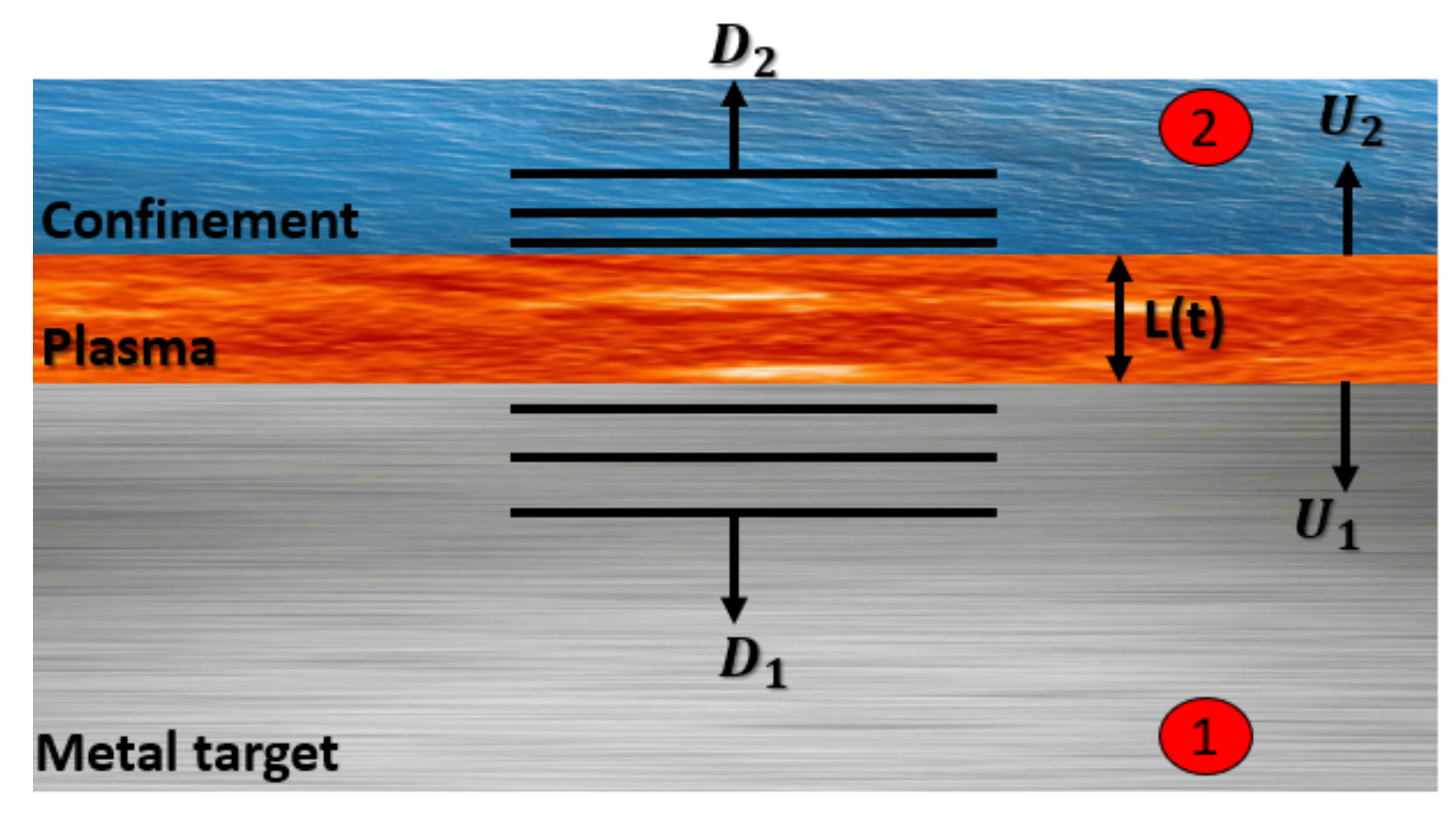
• The laser pulse is absorbed at the boundary between the confinement and the metal where the plasma is created. This plasma then extends in a 1D geometry (the model is said to be mono-dimensional) with two shock waves generated in both the metal and the confinement (see Figure 10).
• The melting and vaporization of the metal is instantaneous. Then, a plasma absorbs all the laser intensity. This plasma is assumed to behave as an ideal gas and a coefficient $\alpha$ is introduced to determine how much of the internal energy $E_i$ of the ideal gas is converted into thermal energy ($\alpha E_i$) or devoted to ionization ($(1-\alpha )E_i$). As no consideration of the plasma is made in this model, the $\alpha$ coefficient must be experimentally determined (from Equation (30)).
• The absorbed laser energy by the ideal gas is assumed to be converted into two parts: the work of the pressure force ($W_P\propto P\mathrm{d}L$, L the thickness of the plasma), and the increase in the internal energy per volume V. ($\mathrm{d}\left[E_{i}V\right]$)
  The work of the pressure force is used to increase the plasma length by pushing both the confinement and the metal target (see Figure 10). Thus, the pressure will depend on the reduced acoustic impedance Z, given by

  $$\frac{2}{Z}=\frac{1}{Z_1}+\frac{1}{Z_2}$$

  (27)

  where $Z_1$ and $Z_2$ are the acoustic impedance of the confinement and the metal, respectively.
• At the end of the laser pulse, the plasma/ideal gas will start to cool down, and the pressure will decrease. This was modeled as a slow adiabatic release which obeys the law of Laplace:

  $$P{V}^{\gamma }=C$$

  (28)

  where P is the plasma pressure, V is its volume and C is a given constant; $\gamma =1+2/3\alpha$ is the adiabatic constant.

One important equation to solve in Fabbro’s model is that of energy conservation, given by

$$I\left(t\right)=\frac{3}{2\alpha }\frac{\mathrm{d}\left[P\right(t\left)L\right(t\left)\right]}{\mathrm{d}t}+P\left(t\right)\frac{\mathrm{dL}\left(\mathrm{t}\right)}{\mathrm{d}t}$$

(29)

A numerical solving of this equation gives access to both the plasma pressure and the plasma thickness.

In the special case of a square laser pulse (constant intensity $I_0$ over a duration $\tau$), one can analytically obtain the maximum reached pressure:

$$P_{max}=\sqrt{\frac{\alpha Z{I}_0}{2\alpha +3}}$$

(30)

Equation (30) clearly shows a dependency of the maximum pressure with both the confinement and the metal properties through the Z parameter. Furthermore, the $\alpha$ coefficient can be obtained by fitting an experimental curve plotting the pressure as a function of the laser intensity.

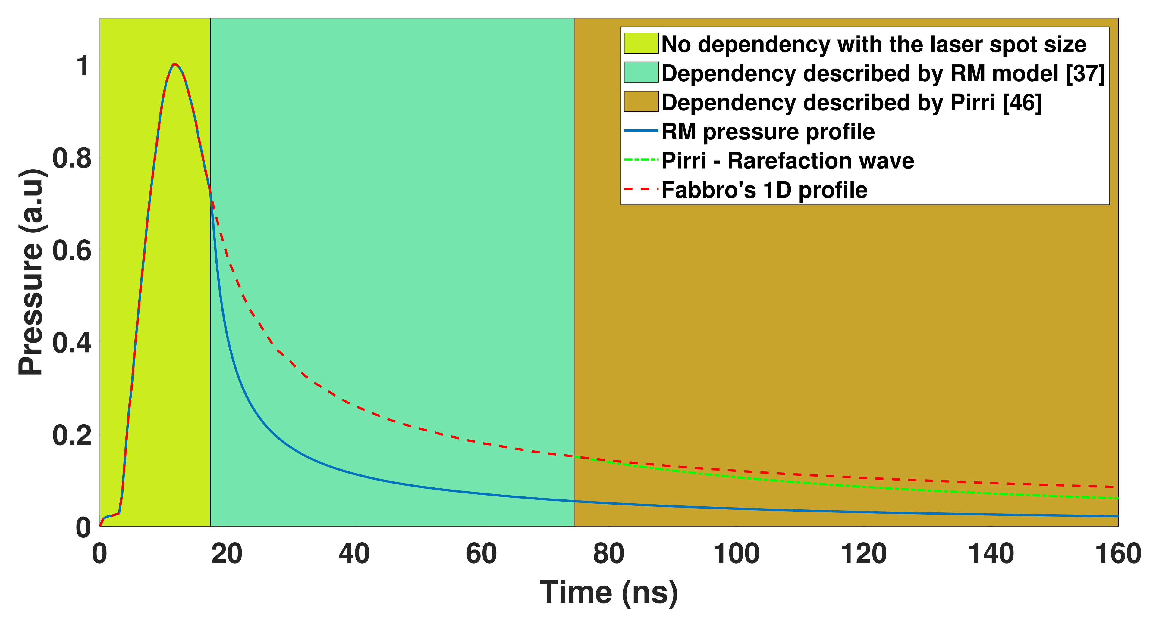
• In 2001, Zhang and Yao proposed a similar approach to Fabbro, with 5-layer geometry: the shocked confinement, the unaffected confinement, the plasma, the unaffected metal and the shocked metal [29,30]. A mass equation conservation was added to obtain the density of the plasma, and the mass flow from the metal and the confinement towards the plasma. Moreover, the rarefaction wave phenomenon described by Pirri [46] was also included in this model to take into account the drop in pressure due to the spherical blast wave generated during the laser pulse. Usually, this phenomenon should be considered over longer time (after the laser pulse), but Zhang was developing a model for micro-scale laser processes, thus resulting in an early apparition of this blast wave.
• In 2003, Sollier et al. proposed an extension of Fabbro’s model named ACCIC [31,36]. Similarly to Zhang and Yao [29,30], a mass conservation equation was included so that the whole involved system of equations can become self-closed. The evaporation of the protective coating layer is considered and calculated based on the Hertz–Knudsen theory. The Thomas–Fermi theory for electrons and Cowan’s theory for ions are applied as the equations of state for the confined plasma, and thermal losses to the work piece target and transparent overlay (water) are taken into account. The confined plasma is considered as a gas of neutrals from the target only, without any contribution from the confining overlay, and the laser absorption coefficient comes from experimental measurements. The rarefaction wave phenomena described by Pirri [46] were also included in this model to take into account the drop in pressure and temperature due to the spherical blast wave generated during the laser pulse. The ACCIC model has been used to compute the thermo-mechanical loading used as input conditions in FEM simulations of the LSP treatment [107].
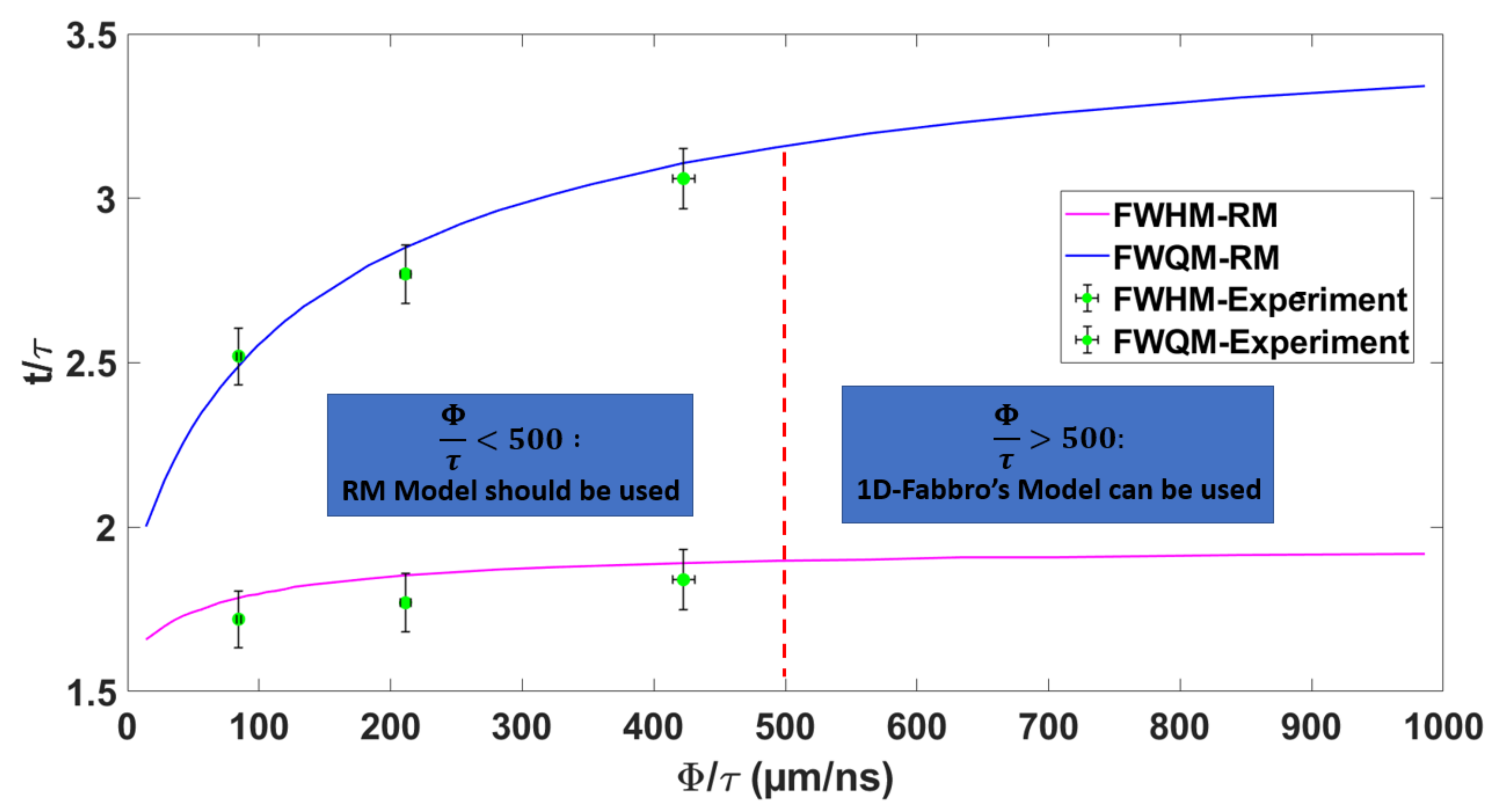
• More recently, it has been experimentally demonstrated that the plasma pressure release was shortened when using small laser spot sizes [37]. Hence, a new model, based on Fabbro’s model, has been proposed, as the previous one was under a mono-dimensional hypothesis which was only valid for large spot sizes. This radius-dependent model (RM) incorporates a plasma-leaking mechanism from the edges, leading to a shortening of the plasma pressure with smaller laser spot sizes. Indeed, this leaking will be proportionally more effective in increasing the plasma volume with small spot sizes, thus resulting in a faster drop of the pressure.

As shown in Figure 11, the full width at half maximum (FWHM) and full width at quarter maximum (FWQM) of the plasma pressure profile (in the case of a square laser pulse) will be reduced regardless of whether the laser spot size decreases or whether the laser pulse duration increases. A criterion was also defined to check whether Fabbro’s model could be used (vertical dashed line).

Finally, in this model, the rarefaction wave of Pirri as a function of the laser spot size and of the plasma temperature was also included.

To summarize the dependency of the plasma pressure profile with the laser spot size, we plotted in Figure 12 a typical laser-induced plasma pressure profile in the confined regime. Three main areas can be identified: the first one (in yellow) for which the pressure profile does not depend on the laser spot size; then, when there is no more laser energy, the pressure profile will decrease more or less quickly depending on the laser spot size (green area): this is the dependency described by the RM model [37]; finally, the last area (in brown) is the arrival of Pirri’s rarefaction wave that creates a drop in the pressure [46].

4.2. Numerical Models

• A first numerical code was developed in the late 1970s by Clauer and their team [108,109,110,111], and was named LILA. This code is based on a finite difference method (FDM) resolution of the differential equations governing hydrodynamic phenomena in the plasma. The absorption of the laser light was calculated for both the cold dense metal and the plasma (through IB absorption). For simplification purposes, a unique equation of state (EOS) was used to describe both the metal and the plasma (taking into account thermal motion and thermal ionization).

Then, the plasma is modeled as an ideal gas of particles (electrons), and the ionization state is determined from Saha’s equation. Finally, equations of conservation of energy, momentum, and mass are added, and the thermal behavior of the plasma (losses by radiative emission and by conduction in the metal) is calculated.

Results obtained by this code, especially the plasma pressure, are in excellent agreement with the experimental results.

• In 2003, Colvin et al. developed a model for low-intensity laser drives which was subsequently incorporated in the 2D radiation-hydrodynamics code LASNEX, in order to simulate the confined laser-matter interaction [112]. The elastic–plastic equations of stress wave propagation were treated in a Lagrangian formulation. The equation of state of all the materials was taken as the analytical quotidian equation of state (QEOS), which is reduces to a Gruneisen EOS at low temperatures. Radiation transport was calculated by multigroup diffusion, with opacities calculated from an average atom model. A ray tracing algorithm simulated laser light propagation through the matter, with inverse Bremsstrahlung absorption on free electrons. The authors also added several prescriptions for calculating:

  •

  The correct ionization state and electron densities for metals and insulators as a function of temperature;

  •

  The low-intensity absorption of the laser beam on a solid or liquid metal;

  •

  The photoionization absorption of the low-intensity laser beam in neutral vapor;

  •

  Collisional ionization, three-body recombination, and dielectric breakdown.

• From 2004 to 2009, Ocaña, Morales and their coworkers developed a simulation model named SHOCKLAS consisting of three principal modules, namely HELIOS, LSPSIM, and HARDSHOCK, which dealt with the main aspects of LSP modeling in a coupled way [113,114,115]. HELIOS is a 1-D radiation-magnetohydrodynamics code which is used to simulate the dynamic evolution of laser-created plasmas. HELIOS solves Lagrangian hydrodynamics equations for a single fluid in which electrons and ions are assumed to be co-moving. Energy transport in the plasma can be treated using either a one-temperature ($T_i=T_e$) model (for both electrons and ions) or a two-temperature ($T_i\ne T_e$) model. Both the electrons and ions are assumed to have Maxwellian distributions defined by their respective temperatures. Material EOS properties are based on either SESAME or PROPACEOS tables, whereas the opacities’ properties are based on tabulated multi-group PROPACEOS data, radiation emission, and absorption terms being coupled to the electron temperature equation. Laser energy deposition is computed using an inverse Bremsstrahlung model, with the restriction that no energy in the beam passes beyond the critical surface.

LSPSIM is a one-dimensional model intended for the estimation of the pressure wave applied to the target material in LSP experiments, similar to those developed by Griffin [116] and Fabbro [28]. It provides a direct input interface for the detailed plasma results obtained by HELIOS for the very beginning of the laser interaction, and for the later times, it provides a time-dependent estimate of the pressure buildup and mechanical target compression when the generated plasma has been exhausted and the shocking dynamics are dominated by gas expansion.

On the basis of the time-dependent pressure profile calculated by HELIOS or LSPSIM, the module HARDSHOCK solves the shock propagation problem into the solid material, with specific consideration of the material response to thermal and mechanical alterations induced by the propagating wave itself. For problems admitting a one-dimensional treatment, the 1D version of HARDSHOCK, which is based on the SWAP-9 code developed at Sandia Laboratories, can be used. For more complicated problems, a 3D version based on the commercial FEM code ABAQUS® is used.

However, there is still a need to compare experimental results to validate these models.

• In 2005, Wu and Shin from Purdue University brought significant improvement in 1D hydrodynamic numerical codes for confined laser-matter interaction [32,117]. Their code adopts a layer geometry (metal/plasma/confinement) to gain a better understanding of how the laser light is transmitted and reflected during the whole interaction. Altogether, the simulated absorption is more accurate. Furthermore, a model for the breakdown is also provided in order to take into account the saturation of intensity reaching the target when a breakdown plasma occurs.

As for the LILA code, a 1D hydrodynamic equation is obtained from the equations of conservation of momentum, mass, and energy. The metal behavior is obtained from a quotidian equation of state (QEOS) which was adapted to high-pressure phenomena.

Finally, the refractive index of the metal (used to calculate the absorption) is obtained from the Drude model and calibrated with experiments.

Similarly to Fabbro’s model, the plasma length is calculated from the material velocity at the interface between the plasma and the metal and between the plasma and the confinement. However, a second mechanism is added to calculate the plasma length: the vaporization and ionization of both the metal and the confinement, which are then incorporated into the plasma.

Later on, they developed a 2D version of their hydrodynamic code [118].

• In 2004, Colombier and Combis [119] from the CEA started developing a 1D Lagrangian hydrodynamic code. This code, currently known as ESTHER, has been recently improved by Videau and Bardy from the CEA [33].

This code provided, for the first time, a complete view of the whole laser shock process: laser interaction with matter, and the propagation of the shock wave in depth of the target.

The geometry considered here is a high number of cells/layers, from the metal to the confinement. The properties of each cell are calculated (mainly the refractive index and the conductivity), and hydrodynamic equations (conservation of momentum, mass, and energy) are calculated as well.

Furthermore, in each cell, the Helmoltz equation is solved and given by

$$△\overrightarrow{E}+\frac{{\omega }^2{n}^2}{c^2}\overrightarrow{E}=0$$

(31)

where $△$ is the Laplacian differential operator, $\overrightarrow{E}$ is the electromagnetic field entering the cell, $\omega$ is the angular frequency, and $n^2$ is the complex refractive index of the cell.

Optical indexes were obtained from tabulated data (Palik tables) for the solid domain, and from a Lorentz-like model in the dense plasma domain [120].

Thermal losses (conductivity, diffusion and radiation) were also calculated, and the thermal constant was obtained from tabulated data.

Today, ESTHER is probably the most effective available code to simulate the whole laser shock process. A lot of parameters may be extracted from the simulation: temperature, pressure, density, and length for every position ranging from the metal to the confinement. Altogether, ESTHER is an accurate code for laser-matter interaction, and it has been optimized based on the most recent and precise experiments conducted.

Indeed, Scius-Bertrand et al. recently compared a set of various experimental parameters (based on different laser sources) [53]. Their results show very good agreement between experimental results and ESTHER’s simulations.

Globally, it provides some normalized temporal profiles and general scaling laws for peak pressures which may then be used as limit conditions for mechanical codes.

However, as ESTHER remains a 1D code, it is hard to reproduce experiments with small laser spot sizes. Furthermore, breakdown phenomena are not included in the laser/matter interaction part, thus making this code only valid for laser intensities under the breakdown threshold intensity.

As previously illustrated in Figure 2, by using the experimental laser intensity (Gaussian pulse) measured as a function of time, the associated plasma pressure simulated using ESTHER code can be plotted.

Finally, in Figure 13 and Figure 14, the estimated temperature and density of the plasma were plotted (both for the aluminum part and the water part), at 20 ns after the laser pulse and with a laser intensity of 1 GW/cm² (Gaussian laser pulse of 7 ns duration at FWHM).

These data may help estimate the plasma length, its temperature, its density, but also the total ablated mass; this is of great importance in understanding the plasma impact on materials. However, experimental data are still required to confirm these last numerical results.

• Most recently, Heya et al. also proposed a 1D code to simulate laser shock interaction [121]. This code, named the integrated simulation code for laser ablation peening (ISLAP), concentrates on the interaction of laser light with the metal target rather than simulating the whole laser shock process. There are three models used in this code: an atomic model, based on a screened hydrogenic model (SHM) and used to obtain the energy levels, population distributions, and ionization states of the metal target; an equation of state (EOS) model to calculate some parameters such as the pressure or the specific heat; and the Cowan model; a laser ablation peening code (LAPCO) to calculate the absorption of the laser light (inverse Bremsstrahlung and resonance absorption) during the process, and also to estimate energy transfers (heating and radiation).

After the first heating and absorption of the laser pulse, the metal target is considered to be under 6 layers/states : solid, solid and liquid, liquid, liquid and neutral gas, neutral gas and partially ionized plasma, and liquid. The water is either neglected for the laser absorption or for being included in the plasma/gas (called a plume by the authors).

However, as for many simulation codes, breakdown phenomena inside the water confinement are not taken into consideration.

5. Applications: Understanding of Laser Shock Generation and Propagation for Aluminum Alloys

The general method we described in the previous part to predict the behavior of materials (especially aluminum alloys) when submitted to strong shock waves in order to become more predictive on the LSP process and residual stresses (and ultimately, fatigue life), have already been explored in previous articles.

In 1996, Peyre et al. conducted a study on various aluminum alloys (A356, Al12Si and Al-7075) [16]. Fabbro’s model was used to estimate the pressure loading applied by each shot on the considered metal sample, and an elastic–plastic model, developed by Ballard [122], was used to estimate the plasticized depth. Residual stresses were evaluated by using the sin²($\Psi$) method (X-ray diffraction) in order to estimate the optimal loading pressure to use. Moreover, fatigue tests were conducted to confirm the previous results and show the effectiveness of LSP treatments on Al alloys. Indeed, a comparison was made to illustrate the enhancement obtained on the fatigue life by the LSP process compared to the one obtained from shot peening.

In a more recent work, Seddik et al. used velocity profiles obtained by VISAR on two aluminum alloys highly used in the aeronautical industry (Al-2024 and Al-7175) to improve numerical simulations [123]. Different constitutive models were used and compared between each other, including the well-known Johnson–Cook model.

Both the temporal distribution of laser energy (Gaussian pulse) and the spatial distribution (smoothed with a DOE), each measured precisely, were implemented on simulations. Hence, the material parameters obtained for Al alloys by fitting experimental velocity profiles and simulated ones are expected to be highly accurate.

It has been shown that better results were obtained with the Johnson–Cook model with a strain hardening law, especially when the shock wave bounces back-and-forth in the metal. However, it was not necessary to use strain hardening for the Al-7175 alloy.

The used material parameters (Hugoniot elastic limit (HEL), deduced from the experimental value of the elastic precursor) and model parameters (the strain hardening modulus K (MPa), the strain hardening parameter $n_h$, the strain rate sensitivity C, and the reference plastic strain rate ${\epsilon }_{p0}$) are summarized in

Table 1. Properties and parameters (Johnson–Cook model) for Al-2024 and Al-7175 alloys [123].

Alloy	${\mathit{P}}_{\mathbf{HEL}}$ (MPa)	K (MPa)	${\mathit{n}}_{\mathit{h}}$	C	${\mathit{\epsilon }}_{\mathit{p}0}$
Al-2024	1028	329	0.35	0.025	0.01
Al-7175	920	0	0	0.01	0.01

.

In a similar work (to be published), Ayad et al. also investigated a Johnson–Cook model for various aluminum alloys: Al-2024, Al-2017, Al-7075, and a FSW (friction stir welding) alloy produced from Al-2017 and Al-7075 [124,125]. A high consistency between experimental velocities (measured by VISAR) and simulated velocities was obtained.

The originality of this research work lies with the fact that shock waves propagation was measured and simulated from two different directions: cross-section (CS) and in-plane (IP), depending on the used cutting plane compared to the rolling direction of the FSW process. These directions were also analyzed from electron back scatter diffraction (EBSD), showing a great difference in the grain size and shapes between CS and IP directions.

Regarding the pressure source term, Fabbro’s model was coupled to Pirri’s rarefaction wave model to estimate the temporal profile, while the spatial profile was reproduced according to image acquisitions from a CCD camera after being smoothened by a DOE. Two spot sizes (3 and 4 mm, to stay close to the 1D case) were used to improve the accuracy of simulation fits, and for the same reason, multiple laser intensities (from 1 to 4 GW/cm²) were set. Finally, edge effects ([103]) were also investigated depending on the spatial shape, at the edges, of the laser beam.

The parameters extracted from fitting experimental signals are summarized in

Table 2. Properties and parameters (Johnson–Cook model) for Al-2024, Al-2017, Al-7075, and FSW (Al2017+Al-7075) alloys [124,125].

Alloy	${\mathit{\sigma }}_{{\mathit{Y}}_0}$ (MPa)	K (MPa)	${\mathit{n}}_{\mathit{h}}$	C
Al-2024	369	329	0.35	0.025
Al-2017 (CS/IP)	260/270	700/350	0.6/0.3	0.035/0.03
Al-7075 (CS/IP)	400/473	800/210	0.45/0.38	0.05/0.033
FSW (2017 + 7075) (CS/IP)	285/340	500/200	0.35/0.2	0.033/0.017

. ${\sigma }_{Y_0}$ is the elastic limit, K is the strain hardening modulus, n is the strain hardening parameter, and C is the strain rate sensitivity.

As simulations become increasingly accurate and show a great ability to reproduce experimental velocities, this indicates that pressure loading terms are well estimated. Further works on aluminum alloys should now concentrate on simulating both residual stresses and fatigue life after LSP treatments, and make a comparison with experimental data.

6. Future Expectations and Improvements

As we demonstrated in this review, a great number of improvements have been made since the discovery of laser shock applications, especially in the last 20 years. However, there are still some challenges and issues to overcome, especially when going towards small laser spot sizes (for specific applications and industrial needs). Indeed, both analytical models and numerical ones are not adapted and must be improved to take into account 2D effects, such as the radial expansion of the plasma. In a previous reference [37], a first model was proposed in agreement with experimental data. However, there are still a lot of phenomena to understand and to experimentally measure, such as the radial leak.

Furthermore, too many experimental data are still required and difficult to obtain, such as plasma temperatures, densities, and optical constants. Even if these data are difficult to obtain, because we showed that confined plasmas are not the easiest to analyze, they shall bring important information to make current models and simulations more accurate.

On the other hand, even if the main mechanisms involved in the breakdown plasma generation are well understood, it remains a challenge to correctly reproduce the experimental values of the breakdown intensity threshold. This shall also help to understand the difference in the behaviors of the surface or the volume.

Finally, concerning the LSP process itself, in order to be more predictive for the thermally affected depth that drives the fatigue performance of treated samples without coating, it remains very important to estimate the thermal source term of the plasma as precisely as possible. Some numerical models such as ESTHER are currently able to provide an estimation of the plasma temperature, but this can also be deduced from the pressure loading term by assuming an ideal gas behavior (thus, the temperature is synchronously varying with the pressure). However, experimental diagnosis (both with a spatial and temporal resolution) should be deployed or improved in order to sharpen our understanding of this matter.

Altogether, the objective will be to couple a well-known pressure loading with the associated thermal loading to fully simulate the LSP process. Thus, this will provide estimations of the thermal and mechanical residual stresses, and hence the fatigue life of treated samples may be anticipated.

7. Conclusions

In this review, the source term of plasmas induced by laser/matter interaction in a confined regime was discussed. The pressure source term was shown to be especially really important for laser shock applications. The main mechanisms which drive the pressure generation were summarized (absorption, breakdown, release), and currently obtained experimental data were reviewed. The wide range of experimental setups available to measure the plasma pressure were presented and their benefits and drawbacks were discussed.

Hence, an historical summary regarding analytical and numerical models was conducted to show the improvements made in the past 50 years; the same review was also conducted regarding the used metrology for experiments. Based on experimental results, analytical and numerical models are becoming more and more predictive and help the laser shock peening process be more effectively applied. This also helps LSP address new applications through new configurations such as LSP without coating.

Future works shall concentrate on measuring the difficult-to-obtain but essential parameters of these plasmas (such as the density and the temperature) in order to obtain improvements either in modeling or in simulations.

References

- Kearton, B.; Mattley, Y. Sparking New Applications. Nat. Photonics 2008, 2, 537–540. [Google Scholar] [CrossRef]
- Meijer, J. Laser beam machining (LBM), state ofthe art and new opportunities. J. Mater. Process. Technol. 2004, 149, 2–17. [Google Scholar] [CrossRef]
- Phipps, C.; Luke, J.; Helgeson, W. Laser space propulsion overview. Proc. SPIE 2007, 6606, 660602. [Google Scholar] [CrossRef]
- Jasim, H.; Demir, A.; Previtali, B.; Taha, Z. Process development and monitoring in stripping of a highly transparent polymeric paint with ns-pulsed fiber laser. Opt. Laser Technol. 2017, 93, 60–66. [Google Scholar] [CrossRef]
- Barletta, M.; Gisario, A.; Tagliaferri, V. Advance in paint stripping from aluminium subtrates. J. Mater. Process. Technol. 2006, 173, 232–239. [Google Scholar] [CrossRef]
- Berthe, L.; Arrigoni, M.; Boustie, M.; Cuq-Lelandais, J.; Broussillou, C.; Fabre, G.; Jeandin, M.; Guipond, V.; Nivard, M. State-of-the-art laser adhesion test (LASAT). Nondestruct. Test. Eval. 2011, 26, 303–317. [Google Scholar] [CrossRef]
- Sagnard, M.; Ecault, R.; Touchard, F.; Boustie, M.; Berthe, L. Development of the symmetrical laser shock test for weak bond inspection. Opt. Laser Technol. 2018, 111, 644–652. [Google Scholar] [CrossRef] [Green Version]
- Furfari, D. Laser Shock Peening to Repair, Design and Manufacture Current and Future Aircraft Structures by Residual Stress Engineering. Adv. Mater. Res. 2014, 891–892, 992–1000. [Google Scholar] [CrossRef]
- Pavan, M. Laser Shock Peening for Fatigue Life Enhancement of Aerospace Components. Ph.D. Thesis, Coventry University, Coventry, UK, 2017. [Google Scholar]
- Sano, Y.; Mukai, N.; Okazaki, K.; Obata, M. Residual stress improvement in metal surface by underwater laser irradiation. Nucl. Instrum. Methods Phys. Res. 1997, B121, 432–436. [Google Scholar] [CrossRef]
- Sano, Y.; Mukai, N.; Yoda, M.; Uehara, T.; Chida, I.; Obata, M. Development and Applications of Laser Peening without Coating as a Surface Enhancement Technology. Proc. SPIE 2006, 6343, 1–12. [Google Scholar] [CrossRef]
- Sano, Y. Quarter Century Development of Laser Peening without Coating. Metals 2020, 10, 152. [Google Scholar] [CrossRef] [Green Version]
- Tenaglia, R.; Lahrman, D. Shock tactics. Nat. Photonics 2009, 3, 267–270. [Google Scholar] [CrossRef]
- Ganesh, P.; Sundar, R.; Kumar, H.; Kaul, R.; Ranganathan, K.; Hedaoo, P.; Tiwari, P.; Kukreja, L.; Oak, S.; Dasari, S.; et al. Studies on laser peening of spring steel for automotive applications. Opt. Laser Eng. 2012, 50, 678–686. [Google Scholar] [CrossRef]
- Sonntag, R.; Reinders, J.; Gibmeier, J.; Kretzer, J. Fatigue Performance of Medical Ti6Al4V Alloy after Mechanical Surface Treatments. Mech. Surf. Treat. FüR Med 2015, 10, 1–15. [Google Scholar] [CrossRef] [Green Version]
- Peyre, P.; Fabbro, R.; Merrien, P.; Lieurade, H.P. Laser shock processing of aluminium alloys. Application to high cycle fatigue behaviour. Mater. Sci. Eng. 1996, A210, 102–113. [Google Scholar] [CrossRef]
- Sano, Y.; Masaki, K.; Gushi, T.; Sano, T. Improvement in fatigue performance of friction stir welded A6061-T6aluminum alloy by laser peening without coating. Mater. Des. 2012, 36, 809–814. [Google Scholar] [CrossRef]
- Kashaev, N.; Ventzke, V.; Horstmann, M.; Chupakhin, S.; Riekehr, S.; Falck, R.; Maawad, E.; Staron, P.; Schell, N.; Huber, N. Effects of laser shock peening on the microstructure and fatigue crack propagation behaviour of thin AA2024 specimens. Int. J. Fatigue 2017, 98, 223–233. [Google Scholar] [CrossRef] [Green Version]
- Peyre, P.; Carboni, C.; Forget, P.; Beranger, G.; Lemaitre, C.; Stuart, D. Influence of thermal and mechanical surface modifications induced by laser shock processing on the initiation of corrosion pits in 316L stainless steel. J. Mater. Sci. 2007, 42, 6866–6877. [Google Scholar] [CrossRef]
- Wang, J.; Zhang, Y.; Chen, J.; Zhou, J.; Ge, M.; Lu, Y.; Li, X. Effects of laser shock peening on stress corrosion behavior of 7075 aluminum alloy laser welded joints. Mater. Sci. Eng. A 2015, 647, 7–14. [Google Scholar] [CrossRef]
- Anderholm, N.C. Laser-generated stress waves. Appl. Phys. Lett. 1970, 16, 113–115. [Google Scholar] [CrossRef]
- Berthe, L.; Fabbro, R.; Peyre, P.; Tollier, L.; Bartnicki, E. Laser shock processing of materials: Study of laser-induced breakdown in water confinement regime. Proc. SPIE 1996, 2789, 246–253. [Google Scholar] [CrossRef]
- Berthe, L.; Fabbro, R.; Peyre, P.; Bartnicki, E. Laser shock processing of materials: Experimental study of breakdown plasma effects at the surface of confining water. Proc. SPIE 1997, 3097, 570–575. [Google Scholar] [CrossRef]
- Berthe, L.; Fabbro, R.; Peyre, P.; Bartnicki, E. Experimental study of the transmission of breakdown plasma generated during laser shock processing. Eur. Phys. J. Appl. Phys. 1998, 3, 215–218. [Google Scholar] [CrossRef]
- Berthe, L.; Fabbro, R.; Peyre, P.; Tollier, L.; Bartnicki, E. Shock waves from a water-confined laser-generated plasma. J. Appl. Phys. 1997, 82, 2826–2832. [Google Scholar] [CrossRef]
- Berthe, L.; Fabbro, R.; Peyre, P.; Bartnicki, E. Wavelength dependent of laser shock-wave generation in the water-confinement regime. J. Appl. Phys. 1999, 85, 7552–7555. [Google Scholar] [CrossRef]
- Berthe, L.; Sollier, A.; Peyre, P.; Fabbro, R.; Bartnicki, E. The generation of laser shock waves in a water-confinement regime with 50 ns and 150 ns XeCl excimer laser pulses. J. Phys. D Appl. Phys. 2000, 33, 2142–2145. [Google Scholar] [CrossRef]
- Fabbro, R.; Fournier, J.; Ballard, P.; Devaux, D.; Virmont, J. Physical study of laser-produced plasma in confined geometry. J. Appl. Phys. 1990, 68, 775–784. [Google Scholar] [CrossRef]
- Zhang, W.; Yao, Y. Microscale Laser Shock Processing—Modeling, Testing, and Microstructure Characterization. J. Manuf. Process. 2001, 3, 128–143. [Google Scholar] [CrossRef]
- Zhang, W.; Yao, Y. Modeling and simulation improvement in laser shock processing. ICALEO 2001, 2001, 59–68. [Google Scholar] [CrossRef] [Green Version]
- Sollier, A.; Berthe, L.; Peyre, P.; Bartnicki, E.; Fabbro, R. Laser-matter interaction in laser shock processing. Proc. SPIE 2003, 4831, 463–467. [Google Scholar] [CrossRef]
- Wu, B.; Shin, Y. A self-closed thermal model for laser shock peening under the water confinement regime configuration and comparisons to experiments. J. Appl. Phys. 2005, 97, 113517. [Google Scholar] [CrossRef]
- Bardy, S.; Aubert, B.; Bergara, T.; Berthe, L.; Combis, P.; Hébert, D.; Lescoute, E.; Rouchausse, Y.; Videau, L. Development of a numerical code for laser-induced shock waves applications. Opt. Laser Technol. 2020, 124, 1–12. [Google Scholar] [CrossRef]
- Peyre, P.; Sollier, A.; Chaieb, I.; Berthe, L.; Bartnicki, E.; Braham, C.; Fabbro, R. FEM simulation of residual stresses induced by laser Peening. Eur. Phys. J. Appl. Phys. 2003, 23, 83–88. [Google Scholar] [CrossRef]
- Hfaiedh, N.; Peyre, P.; Song, H.; Popa, I.; Ji, V.; Vignal, V. Finite element analysis of laser shock peening of 2050-T8 aluminum alloy. Int. J. Fatigue 2015, 70, 480–489. [Google Scholar] [CrossRef] [Green Version]
- Berthe, L.; Sollier, A.; Peyre, P.; Fabbro, R. Study of plasma induced by laser in water confinement regime: Application to laser shock processing with and without thermal protective coating. ICALEO 2003, 2003, 1502. [Google Scholar] [CrossRef]
- Rondepierre, A.; Unaldi, S.; Rouchausse, Y.; Videau, L.; Fabbro, R.; Casagrande, O.; Simon-Boisson, C.; Besaucèle, H.; Castelnau, O.; Berthe, L. Beam size dependency of a laser-induced plasma in confined regime: Shortening of the plasma release. Influence on pressure and thermal loading. Opt. Laser Technol. 2021, 135, 106689. [Google Scholar] [CrossRef]
- Sakka, T.; Takatani, K.; Ogata, Y.; Mabuchi, M. Laser ablation at the solid–liquid interface: Transient absorption of continuous spectral emission by ablated aluminium atoms. J. Phys. D Appl. Phys. 2001, 35, 65–73. [Google Scholar] [CrossRef]
- Kanitz, A.; Kalus, M.R.; Gurevich, E.; Ostendorf, A.; Barcikowski, S.; Amans, D. Review on experimental and theoretical investigations of the early stage, femtoseconds to microseconds processes during laser ablation in liquid-phase for the synthesis of colloidal nanoparticles. Plasma Sources Sci. Technol. 2019, 28, 103001. [Google Scholar] [CrossRef]
- Berthe, L.; Sollier, A.; Peyre, P.; Carboni, C.; Bartnicki, E.; Fabbro, R. Physics of shock-wave generation by laser plasma in water confinement regime. Proc. SPIE 2000, 4065, 511–520. [Google Scholar] [CrossRef]
- Berthe, L.; Sollier, A.; Courapied, D.; Bartnicki, E. Laser interaction in water confinement regime for laser shock processing (LSP): Absorption measurements. ICALEO 2014, 2014, 552–555. [Google Scholar] [CrossRef]
- Max, C. Theory of the coronal plasma in laser-fusion targets. Phys. Laser Fusion 1981, I, 1–78. [Google Scholar] [CrossRef] [Green Version]
- Mora, P. Theoretical model of absorption of laser light by a plasma. Phys. Fluids 1982, 25, 1051–1056. [Google Scholar] [CrossRef]
- Spitzer, L.; Härm, R. Transport Phenomena in a Completely Ionized Gas. Phys. Rev. 1953, 89, 977–981. [Google Scholar] [CrossRef]
- Garban-Labaune, C.; Fabre, E.; Max, C.; Amiranoff, F.; Fabbro, R.; Virmont, J.; Mead, W. Experimental results and theoretical analysis of the effect of wavelength absorption and hot-electron generation in laser-plasma interaction. Phys. Fluids 1985, 28, 2580–2590. [Google Scholar] [CrossRef]
- Pirri, A. Theory for momentum transfer to a surface with a high-power laser. Phys. Fluids 1973, 16, 1435–1440. [Google Scholar] [CrossRef]
- Pirri, A.; Root, R.; Wu, P. Plasma Energy Transfer to Metal Surfaces Irradiated by Pulsed Lasers. AIAA J. 1978, 16, 1296–1304. [Google Scholar] [CrossRef]
- Sollier, A.; Berthe, L.; Fabbro, R. Numerical modeling of the transmission of breakdown plasma generated in water during laser shock processing. Eur. Phys. J. Appl. Phys. 2001, 16, 131–139. [Google Scholar] [CrossRef]
- Wu, B.; Shin, Y. Laser pulse transmission through the water breakdown plasma in laser shock peening. Appl. Phys. Lett. 2006, 88, 041116. [Google Scholar] [CrossRef]
- Kennedy, P. A fist-order model for computation of laser-induced breakdown thresholds in ocular and aqueous media: Part I—Theory. IEEE J. Quantum Electron. 1995, 31, 2241–2250. [Google Scholar] [CrossRef]
- Keldish, L. Ionization in the field of a strong electromagnetic wave. Sov. Phys. JETP 1965, 20, 1307–1314. [Google Scholar]
- Grey Morgan, C. Laser-induced breakdown of gases. Rep. Prog. Phys. 1975, 38, 621–665. [Google Scholar] [CrossRef]
- Scius-Bertrand, M.; Videau, L.; Rondepierre, A.; Lescoute, E.; Rouchausse, Y.; Kaufman, J.; Rostohar, D.; Brajer, J.; Berthe, L. Laser induced plasma characterization in direct and water confined regimes: New advances in experimental studies and numerical modelling. J. Phys. D Appl. Phys. 2020, 54, 055204. [Google Scholar] [CrossRef]
- Rondepierre, A.; Rouchausse, Y.; Videau, L.; Casagrande, O.; Castelnau, O.; Berthe, L. Laser interaction in a water tank configuration: Higher confinement breakdown threshold and greater generated pressures for laser shock peening. J. Laser Appl. 2021, 33. [Google Scholar] [CrossRef]
- Fabbro, R.; Peyre, P.; Berthe, L.; Scherpereel, X. Physics and applications of laser-shock processing. J. Laser Appl. 1998, 10, 265–279. [Google Scholar] [CrossRef]
- Peyre, P.; Carboni, C.; Sollier, A.; Berthe, B.; Richard, C.; de Los Rios, E.; Fabbro, R. New trends in laser shock wave physics and applications. Proc. SPIE 2002, 4760, 654–666. [Google Scholar] [CrossRef]
- Peyre, P. Laser Shock Processing on Metal. Metals 2017, 7, 409. [Google Scholar] [CrossRef] [Green Version]
- Clauer, A. Laser Shock Peening, the Path to Production. Metals 2019, 9, 626. [Google Scholar] [CrossRef] [Green Version]
- Zhang, D.; Gökce, B.; Barcikowski, S. Laser Synthesis and Processing of Colloids: Fundamentals and Applications. Chem. Rev. 2017, 117, 3990–4103. [Google Scholar] [CrossRef]
- Amans, D.; Cai, W.; Barcikowski, S. Status and demand of research to bring laser generation of nanoparticles in liquids to maturity. Appl. Surf. Sci. 2019, 488, 445–454. [Google Scholar] [CrossRef]
- Matsumoto, A.; Sakka, T. A review of underwater laser-induced breakdown spectroscopy of submerged solids. Anal. Sci. 2020, in press. [Google Scholar] [CrossRef]
- Nguyen, T.; Tanabe, R.; Ito, Y. Comparative study of the expansion dynamics of laser-driven plasma and shock wave in in-air and underwater ablation regimes. Opt. Laser Technol. 2018, 100, 21–26. [Google Scholar] [CrossRef]
- Saito, K.; Takatani, K.; Sakka, T.; Ogata, Y. Observation of the light emitting region produced by pulsed laser irradiation to a solid–liquid interface. Appl. Surf. Sci. 2002, 197–198, 56–60. [Google Scholar] [CrossRef]
- Oguchi, H.; Sakka, T.; Ogata, Y. Effects of pulse duration upon the plume formation by the laser ablation of Cu in water. J. Appl. Phys. 2007, 102, 023306. [Google Scholar] [CrossRef] [Green Version]
- Takada, N.; Nakano, T.; Sasaki, K. Influence of additional external pressure on optical emission intensity in liquid-phase laser ablation. Appl. Surf. Sci. 2009, 255, 9572–9575. [Google Scholar] [CrossRef]
- Dell’Aglio, M.; Santagata, A.; Valenza, G.; DeStradis, A.; DeGiacomo, A. Study of the effect of water pressure on plasma and cavitation bubble induced by pulsed laser ablation in liquid of silver and missed variations of observable nanoparticle features. ChemPhysChem 2017, 18, 1165–1174. [Google Scholar] [CrossRef]
- Ilyin, A.; Bukin, O.; Bulanov, A. Regimes of laser plasma expansion at optical breakdown in the normal atmosphere. Tech. Phys. 2008, 53, 693–696. [Google Scholar] [CrossRef]
- Raǐzer, Y.P. Heating of a Gas by a Powerful Light Pulse. Sov. Phys. JETP 1965, 21, 1009–1017. [Google Scholar]
- Sakka, T.; Iwanaga, S.; Ogata, Y.; Matsunawa, A.; Takemoto, T. Laser ablation at solid–liquid interfaces: An approach from optical emission spectra. J. Chem. Phys. 2000, 112, 8645–8653. [Google Scholar] [CrossRef] [Green Version]
- Sakka, T.; Saito, K.; Ogata, Y. Emission spectra of the species ablated from a solid target submerged in liquid: Vibrational temperature of C2 molecules in water-confined geometry. Appl. Surf. Sci. 2002, 197–198, 246–250. [Google Scholar] [CrossRef]
- Saito, K.; Sakka, T.; Ogata, Y. Rotational spectra and temperature evaluation of C2 molecules produced by pulsed laser irradiation to a graphite–water interface. J. Appl. Phys. 2003, 94, 5530–5536. [Google Scholar] [CrossRef] [Green Version]
- Sakka, T.; Saito, K.; Ogata, Y. Confinement effect of laser ablation plume in liquids probed by self-absorption of C2 Swan band emission. J. Appl. Phys. 2005, 97, 014902. [Google Scholar] [CrossRef] [Green Version]
- Sakka, T.; Oguchi, H.; Masai, S.; Hirata, K.; Ogata, Y.; Saeki, M.; Ohba, H. Use of a long-duration ns pulse for efficient emission of spectral lines from the laser ablation plume in water. Appl. Phys. Lett. 2006, 88, 061120. [Google Scholar] [CrossRef] [Green Version]
- Sakka, T.; Yamagata, H.; Oguchi, H.; Fukami, K.; Ogata, Y. Emission spectroscopy of laser ablation plume: Composition analysis of a target in water. Appl. Surf. Sci. 2009, 255, 9576–9580. [Google Scholar] [CrossRef] [Green Version]
- Sakka, T.; Masai, S.; Fukami, K.; Ogata, Y. Spectral profile of atomic emission lines and effects of pulse duration on laser ablation in liquid. Spectrochim. Acta Part B At. Spectrosc. 2009, 64, 981–985. [Google Scholar] [CrossRef] [Green Version]
- Tamura, A.; Matsumoto, A.; Fukami, K.; Nishi, N.; Sakka, T. Simultaneous observation of nascent plasma and bubble induced by laser ablation in water with various pulse durations. J. Appl. Phys. 2015, 117, 173304. [Google Scholar] [CrossRef] [Green Version]
- Matsumoto, A.; Tamura, A.; Honda, T.; Hirota, T.; Kobayashi, K.; Katakura, S.; Nishi, N.; Amano, K.; Fukami, K.; Sakka, T. Transfer of the Species Dissolved in a Liquid into Laser Ablation Plasma: An Approach Using Emission Spectroscopy. J. Phys. Chem. C 2015, 119, 26506–26511. [Google Scholar] [CrossRef]
- Lam, J.; Amans, D.; Chaput, F.; Diouf, M.; Ledoux, G.; Mary, N.; Masenelli-Varlot, K.; Motto-Ros, V.; Dujardin, C. γ-Al2O3 nanoparticles synthesised by pulsed laser ablation in liquids: A plasma analysis. Phys. Chem. Chem. Phys. 2014, 16, 963–973. [Google Scholar] [CrossRef]
- Amans, D.; Chenus, A.C.; Ledoux, G.; Dujardin, C.; Reynaud, C.; Sublemontier, O.; Masenelli-Varlot, K.; Guillois, O. Nanodiamond synthesis by pulsed laser ablation in liquids. Diam. Relat. Mater. 2009, 18, 177–180. [Google Scholar] [CrossRef]
- Kumar, B.; Thareja, R. Synthesis of nanoparticles in laser ablation of aluminum in liquid. J. Appl. Phys. 2010, 108, 064906. [Google Scholar] [CrossRef]
- Kumar, B.; Yadav, D.; Thareja, R. Growth dynamics of nanoparticles in laser produced plasma in liquid ambient. J. Appl. Phys. 2011, 110, 074903. [Google Scholar] [CrossRef]
- Kumar, B.; Thareja, R. Laser ablated copper plasmas in liquid and gas ambient. Phys. Plasmas 2013, 20, 053503. [Google Scholar] [CrossRef]
- De Giacomo, A.; Dell’Aglio, M.; Santagata, A.; Gaudiuso, R.; De Pascale, O.; Wagener, P.; Messina, G.C.; Compagnini, G.; Barcikowski, S. Cavitation dynamics of laser ablation of bulk and wire-shaped metals in water during nanoparticles production. Phys. Chem. Chem. Phys. 2013, 15, 3083–3092. [Google Scholar] [CrossRef] [PubMed]
- Dell’Aglio, M.; Gaudiuso, R.; DePascale, O.; DeGiacomo, A. Mechanisms and processes of pulsed laser ablation in liquids during nanoparticle production. Appl. Surf. Sci. 2015, 348, 4–9. [Google Scholar] [CrossRef]
- Amans, D.; Diouf, M.; Lam, J.; Ledoux, G.; Dujardin, C. Origin of the nano-carbon allotropes in pulsed laser ablation in liquids synthesis. J. Colloid Interface Sci. 2017, 489, 114–125. [Google Scholar] [CrossRef] [PubMed]
- Shih, C.Y.; Shugaev, M.; Wu, C.; Zhigilei, L. Generation of Subsurface Voids, Incubation Effect, and Formation of Nanoparticles in Short Pulse Laser Interactions with Bulk Metal Targets in Liquid: Molecular Dynamics Study. J. Phys. Chem. C 2017, 121, 16549–16567. [Google Scholar] [CrossRef] [PubMed] [Green Version]
- Shih, C.Y.; Wu, C.; Shugaev, M.; Zhigilei, L. Atomistic modeling of nanoparticle generation in short pulse laser ablation of thin metal films in water. J. Colloid Interface Sci. 2017, 489, 3–17. [Google Scholar] [CrossRef] [PubMed] [Green Version]
- Shugaev, M.; Shih, C.Y.; Karim, E.; Wu, C.; Zhigilei, L. Generation of nanocrystalline surface layer in short pulse laser processing of metal targets under conditions of spatial confinement by solid or liquid overlayer. Appl. Surf. Sci. 2017, 417, 54–63. [Google Scholar] [CrossRef]
- Romain, J.P.; Zagouri, D. Laser-shock studies using an electromagnetic gauge for particle velocity measurements. In Shock Compression of Condensed Matter–1991; Schmidt, S., Dick, R., Forbes, J., Tasker, D., Eds.; Elsevier: Amsterdam, The Netherlands, 1992; pp. 801–804. [Google Scholar] [CrossRef]
- Peyre, P.; Fabbro, R. Electromagnetic Gauge Study of Laser-Induced Shock Waves in Aluminium Alloys. J. Phys. III France 1995, 5, 1953–1964. [Google Scholar] [CrossRef]
- Peyre, P.; Berthe, L.; Fabbro, R.; Sollier, A. Experimental determination by PVDF and EMV techniques of shock amplitudes induced by 0.6–3 ns laser pulses in a confined regime with water. J. Phys. D Appl. Phys. 2000, 33, 498–503. [Google Scholar] [CrossRef]
- Romain, J.; Bauer, F.; Zagouri, D.; Boustie, M. Measurement of laser induced shock pressures using PVDF gauges. AIP Conf. Proc. 1994, 309, 1915–1918. [Google Scholar] [CrossRef]
- Boustie, M.; Couturier, S.; Zagouri, D.; Simonnet, H. Shock pressure and free surface velocity measurements in confined interaction—Response of new VF2/VF3 piezoelectric gauges. Laser Part. Beams 1996, 14, 171–179. [Google Scholar] [CrossRef]
- Strand, O.; Goosman, D.; Martinez, C.; Whitworth, T.; Kuhlow, W. Compact system for high-speed velocimetry using heterodyne techniques. Rev. Sci. Instruments 2006, 77, 083108. [Google Scholar] [CrossRef]
- Dolan, D. Extreme measurements with Photonic Doppler Velocimetry (PDV). Rev. Sci. Instruments 2020, 91, 051501. [Google Scholar] [CrossRef] [PubMed]
- Dolan, D. Accuracy and precision in photonic Doppler velocimetry. Rev. Sci. Instruments 2010, 81, 053905. [Google Scholar] [CrossRef] [Green Version]
- Valenzuela, A.; Rodriguez, G.; Clarke, S.; Thomas, K. Photonic Doppler Velocimetry of laser-ablated ultrathin metals. Rev. Sci. Instruments 2007, 78, 013101. [Google Scholar] [CrossRef]
- Mercier, P.; Bénier, J.; Frugier, P.; Sollier, A.; Le Gloahec, M.R.; Lescoute, E.; Cuq-Lelandais, J.P.; Boustie, M.; de Rességuier, T.; Claverie, A.; et al. PDV measurements of ns and fs laser driven shock experiments on solid targets. AIP Conf. Proc. 2009, 1195, 581–584. [Google Scholar] [CrossRef]
- Nissim, N.; Greenberg, E.; Werdiger, M.; Horowitz, Y.; Bakshi, L.; Ferber, Y.; Glam, B.; Fedotov-Gefen, A.; Perelmutter, L.; Eliezer, S. Free-surface velocity measurements of opaque materials in laser-driven shock-wave experiments using photonic Doppler velocimetry. Matter Radiat. Extrem. 2021, 6, 046902. [Google Scholar] [CrossRef]
- Bovid, S.; Clauer, A.; Kattoura, M.; Vivek, A.; Daehn, G.; Niezgoda, S. Measurement and characterization of nanosecond laser driven shockwaves utilizing photon Doppler velocimetry. J. Appl. Phys. 2021, 129, 205101. [Google Scholar] [CrossRef]
- Barker, L.; Hollenbach, R. Laser interferometer for measuring high velocities of any reflecting surface. J. Appl. Phys. 1972, 43, 4669–4675. [Google Scholar] [CrossRef]
- Thomas, W.; Threadgill, P.; Nicholas, E. Feasibility of friction stir welding steel. Sci. Technol. Weld. Join. 1999, 4, 365–372. [Google Scholar] [CrossRef]
- Boustie, M.; Cuq-Lelandais, J.; Berthe, L.; Bolis, C.; Barradas, S.; Arrigoni, M.; De Resseguier, T.; Jeandin, M. Damaging of material by bi-dimensional dynamic effects. AIP Conf. Proc. 2007, 955, 1323–1326. [Google Scholar] [CrossRef]
- Boustie, M.; Cuq-Lelandais, J.; Bolis, C.; Berthe, L.; Barradas, S.; Arrigoni, M.; de Resseguier, T.; Jeandin, M. Study of damage phenomena induced by edge effects into materials under laser driven shocks. J. Phys. D Appl. Phys. 2007, 40, 7103–7108. [Google Scholar] [CrossRef]
- Johnson, G.; Cook, W. A constitutive model and data for materials subjected to large strains, high-strain rates and high temperatures. In Proceedings of the 7th International Symposium on Ballistics, The Hague, The Netherlands, 19–21 April 1983; pp. 541–547. [Google Scholar]
- Radziejewska, J.; Strzelec, M.; Ostromski, R.; Sarzynski, A. Experimental investigation of shock wave pressure induced by a ns laser pulse under varying confined regimes. Opt. Laser Eng. 2019, 126. [Google Scholar] [CrossRef]
- Peyre, P.; Chaieb, I.; Braham, C. FEM calculation of residual stresses induced by laser shock processing in stainless steels. Model. Simul. Mater. Sci. Eng. 2007, 15, 205–221. [Google Scholar] [CrossRef]
- Fairand, B.; Clauer, A.; Jung, R.; Wilcox, B. Quantitative assessment of laser-induced stress waves generated at confined surfaces. Appl. Phys. Lett. 1974, 25, 431–433. [Google Scholar] [CrossRef]
- Fairand, B.; Clauer, A. Laser generation of high-amplitude stress waves in materials. J. Appl. Phys. 1979, 50, 1497–1502. [Google Scholar] [CrossRef] [Green Version]
- Fairand, B.; Clauer, A. Laser generated stress waves: Their characteristics and their effects to materials. AIP Conf. Proc. 1979, 50, 27–42. [Google Scholar] [CrossRef] [Green Version]
- Clauer, A.; Holbrook, J.; Fairand, B. Effects of Laser Induced Shock Waves on Metals. In Shock Waves and High-Strain-Rate Phenomena in Metals: Concepts and Applications; Springer: Boston, MA, USA, 1981; pp. 675–702. [Google Scholar] [CrossRef]
- Colvin, J.; Ault, E.; King, W.; Zimmerman, I. Computational model for a low-temperature laser-plasma driver for shock-processing of metals and comparison to experimental data. Phys. Plasmas 2003, 10, 2940–2947. [Google Scholar] [CrossRef]
- Ocaña, J.; Morales, M.; Molpeceres, C.; Torres, J. Numerical simulation of surface deformation and residual stresses fields in laser shock processing experiments. Appl. Surf. Sci. 2004, 238, 242–248. [Google Scholar] [CrossRef]
- Morales, M.; Ocaña, J.; Molpeceres, C.; Porro, J.; García-Beltrán, A. Model based optimization criteria for the generation of deep compressive residual stress fields in high elastic limit metallic alloys by ns-laser shock processing. Surf. Coatings Technol. 2008, 202, 2257–2262. [Google Scholar] [CrossRef] [Green Version]
- Morales, M.; Porro, J.; Blasco, M.; Molpeceres, C.; Ocaña, J. Numerical simulation of plasma dynamics in laser shock processing experiments. Appl. Surf. Sci. 2009, 255, 5181–5185. [Google Scholar] [CrossRef]
- Griffin, R.; Justus, B.; Campillo, A.; Goldberg, L. Interferometric studies of the pressure of a confined laser-heated plasma. J. Appl. Phys. 1986, 59, 1968–1971. [Google Scholar] [CrossRef]
- Wu, B.; Shin, Y. A one-dimensional hydrodynamic model for pressures induced near the coating-water interface during laser shock peening. J. Appl. Phys. 2007, 101, 023510. [Google Scholar] [CrossRef]
- Wu, B.; Shin, Y. Two dimensional hydrodynamic simulation of high pressures induced by high power nanosecond laser-matter interactions under water. J. Appl. Phys. 2007, 101, 103514. [Google Scholar] [CrossRef]
- Colombier, J.; Combis, P.; Bonneau, F.; Le Harzic, R.; Audouard, E. Hydrodynamic simulations of metal ablation by femtosecond laser irradiation. Phys. Rev. B 2005, 71, 165406. [Google Scholar] [CrossRef] [Green Version]
- Faussurier, G.; Blancard, C.; Combis, P.; Decoster, A.; Videau, L. Electronic transport coefficients in plasmas using an effective energy-dependent electron-ion collision-frequency. Phys. Plasmas 2017, 24. [Google Scholar] [CrossRef]
- Heya, M.; Furukawa, H.; Tsuyama, M.; Nakano, H. Simulations of the effects of laser wavelength, pulse duration, and power density on plume pressure generation using a one-dimensional simulation code for laser shock processing. J. Appl. Phys. 2021, 129, 1–21. [Google Scholar] [CrossRef]
- Ballard, P. Contraintes réSiduelles Induites par Impact Rapide. Application au Choc-Laser. Ph.D. Thesis, Ecole Polytechnique, Palaiseau, France, 1991. Available online: https://pastel.archives-ouvertes.fr/pastel-00001897 (accessed on 7 November 2021).
- Seddik, R.; Rondepierre, A.; Prabhakaran, S.; Morin, L.; Favier, V.; Palin-Luc, T.; Berthe, L. Identification of constitutive equations at very high strain rates using shock wave produced by laser. Eur. J. Mech. A Solids 2021, 92, 104432. [Google Scholar] [CrossRef]
- Ayad, M.; Rondepierre, A.; Lapostolle, L.; Le Bras, C.; Unaldi, S.; Trdan, U.; Rouchausse, Y.; Grassy, J.; Maillot, T.; Berthe, L. High Strain Rate Laser Shock Propagation through Aluminum Alloys. 2021; in press. [Google Scholar]
- Ayad, M.; Berthe, L.; Rondepierre, A.; Donik, C.; Klobcar, D.; Trdan, U. Material Model Characterization of Dissimilar 7075-2017 Friction stir Welded Aluminum Alloy Joint under High-Strain Rate Shock Loading. 2021; in press. [Google Scholar]