On the Performance of One-Stage and Two-Stage Object Detectors in Autonomous Vehicles Using Camera Data

Abstract

Object detection using remote sensing data is a key task of the perception systems of self-driving vehicles. While many generic deep learning architectures have been proposed for this problem, there is little guidance on their suitability when using them in a particular scenario such as autonomous driving. In this work, we aim to assess the performance of existing 2D detection systems on a multi-class problem (vehicles, pedestrians, and cyclists) with images obtained from the on-board camera sensors of a car. We evaluate several one-stage (RetinaNet, FCOS, and YOLOv3) and two-stage (Faster R-CNN) deep learning meta-architectures under different image resolutions and feature extractors (ResNet, ResNeXt, Res2Net, DarkNet, and MobileNet). These models are trained using transfer learning and compared in terms of both precision and efficiency, with special attention to the real-time requirements of this context. For the experimental study, we use the Waymo Open Dataset, which is the largest existing benchmark. Despite the rising popularity of one-stage detectors, our findings show that two-stage detectors still provide the most robust performance. Faster R-CNN models outperform one-stage detectors in accuracy, being also more reliable in the detection of minority classes. Faster R-CNN Res2Net-101 achieves the best speed/accuracy tradeoff but needs lower resolution images to reach real-time speed. Furthermore, the anchor-free FCOS detector is a slightly faster alternative to RetinaNet, with similar precision and lower memory usage.

1. Introduction

The increase in availability and quality of remote sensing data provided by modern multi-modal sensors has allowed pushing the state-of-the-art in many computer vision tasks. The data provided by high-resolution cameras and proximity sensors have helped to develop more powerful machine learning models that have achieved unprecedented results in visual recognition problems [1]. These developments have significantly improved the perception systems used in many applications such as autonomous driving [2,3], security surveillance [4], or land monitoring [5]. In recent years, autonomous vehicles are attracting increasing attention given their potential to improve road safety and traffic congestions, while also reducing harmful emissions [6]. However, the accurate perception of the multiple traffic participants (cars, bikes, pedestrians, traffic signs, etc.) that interact with a vehicle still remains a challenging task.

Current efforts in the autonomous driving community focus on building a reliable Advanced Driver-Assistance System (ADAS) that captures information about the environment through many on-board sensors (RGB cameras, LiDAR, GPS, etc.). One of the essential tasks that an ADAS needs to address is object detection. These remote sensing systems need to detect traffic targets in real time in order to make informed driving decisions. Furthermore, they have to be robust enough to operate effectively in complex scenarios such as adverse weather, poor lighting, or occluded objects. These requirements present difficulties that still prevent self-driving vehicles from operating safely in real-world environments. Research in this field is mainly based on the use of RGB images and LiDAR data, which are often fused to improve the reliability of the system. However, due to the high cost of the LiDAR hardware, camera-based systems are increasing their popularity [7]. Camera data is inexpensive, needs less memory usage, and is faster to process than LiDAR 3D point clouds [8].

In this study, we aim to explore the performance of existing 2D object detection models on a multi-class problem (vehicles, pedestrians, and cyclists), using images obtained from the on-board cameras of an autonomous vehicle. In recent years, significant advances in object detection problems were achieved due to the development of deep learning (DL) architectures based on convolutional neural networks (CNNs). Many DL detection frameworks were proposed, such as Faster R-CNN [9], Single Shot Detector (SSD) [10] which is also known as RetinaNet, You Only Look Once (YOLO) [11], or the Fully Convolutional One-Stage Detector (FCOS) [12]. If we only consider accuracy results, these models were applied successfully to general-purpose benchmark datasets such as COCO [13]. However, they present limitations when applied to real-time applications such as autonomous driving. Apart from detection accuracy, other aspects are essential in this scenario, such as the required computational resources and the inference speed. With the many different existing architectures, it is difficult for practitioners to find out which is the most suitable for this particular problem. At a high level, existing deep learning architectures to detect objects with remote sensing camera data present a common methodology: a convolutional backbone as a feature extractor and a sliding window style prediction with a mixed regression and classification objective. This allows performing a unified comparison between a large number of detection systems with different configurations [14].

The experimental study carried out in this work evaluates and compares the performance of four detection meta-architectures using different feature extractors and image resolutions. Given that state-of-the-art detectors are commonly divided into two families (one-stage and two-stage), we have selected the most representative members of each family in order to analyze their different characteristics. We study the combination of one-stage (RetinaNet, FCOS, YOLOv3) and two-stage (Faster R-CNN) meta-architectures with different feature extractors (ResNet-50, ResNet-101, ResNet-152, ResNeXt-101, Res2Net-101, DarkNet-53, MobileNet V1, MobileNet V2). Furthermore, we perform experiments with the camera images at the original high resolution and with reduced resolution. These combinations comprise a total of 30 different models, which were trained using transfer learning. The models are fine-tuned from publicly available models that were pre-trained with the COCO dataset. Transfer learning allows adapting models from other domains to our problem, avoiding the excessive time and resources required to train very deep CNNs from scratch [15]. For the experiments, we use the Waymo Open Dataset [16], which is the most extensive and diverse benchmark up to date. An online competition was recently hosted with this dataset, but only considering the detection accuracy and ignoring the computational efficiency of the proposed methodologies. For this reason, we aim to provide a full picture of the speed/accuracy trade-off by exploring several models with different settings.

To the best of our knowledge, no other studies analyze multi-class object detection in autonomous vehicles with camera data by evaluating different factors such as accuracy, speed, and memory usage of several deep learning models. In summary, the main contributions of this work are as follows:

• A review of the main deep learning meta-architectures and feature extractors for 2D object detection.
• An evaluation of Faster R-CNN, RetinaNet, YOLO and FCOS architectures over several performance metrics in the context of autonomous vehicles.
• An exhaustive analysis of the influence of different backbone networks and image resolutions in the speed/accuracy trade-off of the models.

The rest of the paper is organized as follows: Section 2 reviews relevant related work; Section 3 presents the materials and the methods proposed in the study; Section 4 presents the results obtained from the experimental study and discusses the main findings; Section 5 presents the conclusions and potential future work.

2. Related Work

Over the last decade, significant advances have been achieved in computer vision thanks to the development of deep learning-based techniques. The increase in computing capacity of modern GPUs has allowed researchers to design very deep convolutional neural networks, which have proven to be the most effective method for extracting useful information from images [17]. For the object detection problem, CNNs have also become the reference method in the literature. The object detection task is a dual problem that consists of the recognition and localization of objects. For this task, the state-of-the-art models can be divided into two categories: two-stage and one-stage detectors. In general terms, two-stage detectors tend to obtain higher accuracy, but with a higher computational cost than one-stage detectors. However, this fact highly depends on the selected convolutional backbone network and the hyperparameter configuration, which is a complex procedure.

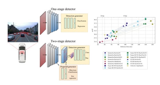
2.1. Two-Stage Detectors

Two-stage frameworks divide the detection process into the region proposal and the classification stage. These models first propose several object candidates, known as regions of interest (RoI), using reference boxes (anchors). In the second step, the proposals are classified and their localization is refined. In R-CNN [18], the pioneering deep learning-based work, an external selective search was used to generate proposals that are fed to a CNN to perform classification and bounding box regression. Later, Faster-RCNN proposed a scheme in which features are shared between both stages, achieving a significant efficiency improvement [9]. Faster R-CNN uses a convolutional backbone network, such as VGG [19] or ResNet [20], which outputs global feature maps. These convolutional maps are shared between the Region Proposal Network (RPN) and the detection network, which reduces the cost of generating proposals externally. Faster R-CNN has inspired many follow-up works that have tried to improve detection accuracy with different approaches, such as designing better backbones that can obtain richer representations. For instance, feature pyramid networks (FPN) were proposed in order to crop RoI features from different levels depending on the scale [21]. Later works have tried to enhance the internal connections of residual networks to better exploit the multi-scale properties of convolutional maps, such as the ResNeXt with grouped convolutions [22] or the Res2Net [23]. Other studies have enhanced the quality of detection by proposing modifications to the existing Faster R-CNN framework. Cascade R-CNN proposes to concatenate several detectors that are trained with increasing intersection-over-union (IoU) thresholds [24]. This architecture can achieve more reliable detections, but increases the required computation, hence being less convenient for real-time applications.

2.2. One-Stage Detectors

On the other hand, one-stage detectors contain a single feed-forward fully convolutional network that directly provides the bounding boxes and the object classification. The Single Shot MultiBox Detector (SSD) [10] and YOLO (You Only Look Once) [11] were among the first to propose a single unified architecture, without requiring a per-proposal computation. However, the extreme foreground-background imbalance in the images prevented these one-stage models from achieving high accuracy. RetinaNet tried to solve this problem by modifying the loss function used in the SSD architecture [25]. RetinaNet also uses FPN and proposes a novel focal loss function that down-weights the importance of easy samples in order to focus on difficult objects. Furthermore, specific lightweight backbone networks that focus on maximizing speed were developed for this architecture, such as MobileNets [26].

YOLO detectors are another anchor-based alternative that divides the image into regions and predict bounding boxes and probabilities for each region. YOLO networks have proved to achieve faster inference rates than RetinaNet, although not being as accurate. However, YOLOv3 was able to enhance detection accuracy by including multi-scale predictions and a better backbone network, DarkNet-53, which uses residual blocks and skip connections [27]. DarkNet-53 is much more powerful than the previous DarkNet-19 and still more efficient than ResNet backbones.

More recently, another popular approach has been to design anchor-free one-stage detectors that do not rely on pre-defined anchor boxes. For instance, FCOS [12] aims to simplify the object detection problem by using the center point of objects to define positives and then predicts the four distances that build the bounding box. FCOS can outperform RetinaNet while being more simple and flexible, eliminating the need for carefully designing anchor boxes for each problem. Other methods such as CornerNet [28] or ExtremeNet [29] first locate several keypoints (e.g., top-left corner and bottom-right corner) and then generate bounding boxes to detect objects. However, these keypoint-based methods require much more complicated post-processing and are considerably slower.

2.3. Object Detection in Autonomous Vehicles

In recent years, the interest in autonomous vehicles has risen. Many datasets have been publicly released, which provides a unique opportunity for researchers to improve the state-of-the-art. In [30], the authors provide a comprehensive overview of the existing autonomous driving datasets and review the most relevant methodologies proposed for detection and segmentation problems. For many years, KITTI was the reference benchmark in the field [31]. More recently, datasets with higher quality and diversity were released, such as PandaSet [32], NuScenes [33], or Waymo [16]. These companies organize online challenges with these datasets for detection problems. However, the main focus is on maximizing accuracy, ignoring the computational efficiency of the proposals, which is extremely important in this context. Besides these challenges, there are several works that addressed detection tasks in the context of autonomous vehicles. In [34], several state-of-the-art models for traffic sign detection were evaluated. An anchor generation optimization procedure to improve vehicle detection was presented in [8]. Other studies provided insights on how to adapt convolutional networks to achieve better performance on pedestrian detection [35]. All these works present different models that are highly tuned for a specific task. However, there is the need to find out general guidelines on which models are best suited for 2D on-board object detection, in which real-time speed is crucial.

3. Materials and Methods

In this section, we present the Waymo dataset and the methodology proposed for the experimental study. Firstly, we review the characteristics of the selected meta-architectures and feature extractors. Finally, we describe the experimental setup and training procedure.

3.1. Waymo Open Dataset

For this study, we selected the recently released Waymo Open Dataset [16], which contains more than a thousand driving scenes recorded across different urban areas. It is the most diverse dataset of this field up to date, in terms of both different locations and weather conditions. Furthermore, Waymo has recently hosted an online challenge on detection over the dataset. The website is still open for submissions, hence novel proposals can be validated. However, the competition only evaluates the accuracy, without considering the efficiency of the models. The dataset contains independently generated labels for three-dimensional LiDAR and two-dimensional camera data. In this study, we focus on the 2D object detection task with the images obtained from the five on-board cameras of the vehicle. Waymo’s vehicle has three frontal cameras with a resolution of $1920\times 1280$, and two lateral cameras with a resolution of $1920\times 886$. Figure 1 displays two example images from the dataset.

The 2D object detection task in this dataset is a multi-class problem with three different types of objects: vehicles, pedestrians, and cyclists.

Table 1. Distribution of object instances in the training and validation sets.

		Training		Validation		Total
Images		74,420	(75%)	24,770	(25%)	99,190
Objects	Vehicle	589,583	(87.9%)	256,076	(91.7%)	845,659	(89.0%)
	Pedestrian	77,569	(11.5%)	21,678	(7.8%)	99,247	(10.5%)
	Cyclist	3842	(0.6%)	1332	(0.5%)	5174	(0.5%)
	Total Objects	670,994	(71%)	279,086	(29%)	950,080

presents the number of images in each set and the label distribution across the three classes. The training and testing division is directly provided by Waymo when downloading the dataset. The dataset contains around 100,000 images in total with almost one million manually annotated objects. As can be seen, the distribution of objects is highly imbalanced. The number of pedestrians and cyclists is significantly lower than the number of vehicles. In this dataset, the 2D bounding box labels are tight-fitting, covering only the visible parts of the objects.

3.2. Deep Learning Meta-Architectures

In this section, we describe the four state-of-the-art meta-architectures with different approaches that are used in this study: Faster R-CNN, RetinaNet, YOLOv3 and FCOS. Faster R-CNN is the most representative model from the two-stage family, while RetinaNet and YOLOv3 are the most widely used anchor-based one-stage architectures [30]. Furthermore, we also evaluate FCOS as an anchor-free alternative to traditional one-stage detectors. Figure 2 illustrates the main differences between two-stage and one-stage approaches at a high-level, providing a more detailed description in the following subsections. As can be seen, two-stage architectures divide the process into the region proposal stage and the classification stage. In contrast, one-stage detectors directly infer the detected boxes. For simplicity, Figure 2 displays the detection process using a single-scale feature map from the backbone network. However, it must be noted that the studied detectors integrate feature pyramid networks in order to detect objects at multiple scales, hence maps with different resolutions are used to generate proposals.

3.2.1. Faster R-CNN

Faster R-CNN is a widely used architecture that follows a multi-task learning procedure, combining classification and bounding box regression to solve the detection problem. This framework uses a convolutional backbone to extract high-level features from the images and consists of two stages: a region proposal network (RPN) and a Fast R-CNN header network [9].

In the first stage, the RPN uses a convolutional sliding window approach over the feature maps extracted by the backbone network to generate proposals. Multi-scale reference boxes (known as anchors) are used at each location of the feature map to predict multiple candidate object boxes. To detect objects at different scales and shapes, the anchors are defined with multiple scales and aspect ratios. The generated proposals pass through a fully connected network that computes the bounding box regression and the objectness score (foreground object vs. background). Afterwards, the top-ranked object candidates are cropped using a RoI (Region of Interest) pooling layer from the same intermediate layer of the feature extractor. A final classification and box-refinement operation are performed for each proposal in the second stage.

The design of multi-scale anchors of this network is a core element for sharing features without extra cost for detecting objects at different scales. Compared to previous approaches in the R-CNN family, the convolutional feature maps are shared between both stages, which enables nearly cost-free region proposals and an end-to-end training procedure. However, since the computation of the second-stage network is run once per each proposal, the candidates provided by the RPN must be limited to a certain number. This is a parameter that must be carefully chosen, as it has a significant influence on the performance of the network, in both accuracy and speed. A larger number of candidates from the RPN may lead to more accurate detections but with a higher inference time, which is undesirable in this context. The typical value used in the original paper is 300 proposals. Furthermore, Faster R-CNN uses non-maximum suppression (NMS) to reduce redundancy within proposals. The NMS procedure is done in both stages and uses an intersection-over-union (IoU) threshold (typically fixed at 0.7) to remove redundant overlapping boxes.

3.2.2. RetinaNet

The RetinaNet is an object detection architecture based on the Single Shot Detector (SSD) that predicts classes and box offsets using a single feed-forward convolutional network [10]. Unlike R-CNN detectors, SSD does not need the second stage of the region proposal network. This fact can lead to faster inference speed since the SSD does not require per-proposal computations. Furthermore, SSD introduces some improvements to compensate for the lack of the second-stage network such as the use of feature maps of different resolutions and default anchor boxes with varying scales and aspect ratios.

This architecture uses a convolutional backbone for feature extraction followed by a feature pyramid network (FPN) which generates multi-scale higher-quality feature maps. The FPN introduces top-down and lateral connections to the extracted maps at different levels in order to build stronger semantic features. Then, SSD divides the image using a grid and assigns pre-defined anchors to each grid cell. This is done for every feature map in the pyramid, allowing SSD to handle objects with different sizes: higher resolution layers for small objects and lower resolution layers for larger ones. A mobile variant of this process, named FPNLite, was presented in [36]. FPNLite allows reducing training parameters and computational cost by replacing the standard convolutions with separable convolutions in the prediction layers.

The original SSD model claimed to outperform two-stage detectors in terms of computational time but was unable to reach the same level of detection accuracy. This performance drop was strongly related to the foreground-background class imbalance present in the image data, with most of the pixels of the images considered as background. Therefore, the number of anchors assigned to objects is very small and the learning process is dominated by background samples. RetinaNet introduced the use of focal loss training to address this problem [25]. The focal loss consists of a weighted loss that down-weights the easy examples and focuses more on training with the hard ones. It is performed using a modulating factor that reduces the loss of easy examples increasing the importance of correcting misclassified examples. The experimental study carried out in [25] proves the improvement of SSD architectures using focal loss, maintaining the speed and outperforming two-stage detectors in terms of accuracy. In this work, all the experiments involving SSD models use the RetinaNet version, hence both terms are indistinctly used.

3.2.3. YOLOv3

YOLOv3 is an improved version over previous YOLO networks that have been widely used for real-time detection [27]. The idea behind YOLO is to divide the image into cells using a grid, which allows achieving faster inference rates. If the center of an object is in a certain grid cell, that cell is responsible for detecting that object. YOLO considers object detection as a regression problem, which means that each cell uses several pre-defined anchor boxes to simultaneously predict the bounding box offsets, the confidence scores, and the class probabilities. The prior anchor box dimensions are obtained with K-means clustering over the training ground truth boxes using a distance metric based on IoU scores [11]. To avoid predictions from diverging too much from the center location, the boxes are calculated as offsets from the obtained cluster centroids.

Compared to previous versions, YOLOv3 presents several improvements such as multi-scale detection, stronger backbone network, and changes in the loss function. In YOLO v3, the predictions are obtained using $1\times 1$ kernels on three feature maps of different scales at different stages of the backbone network. Therefore, more bounding boxes per image are generated. Instead of applying 5 anchor boxes at the last feature map, YOLOv3 generates 9 anchor boxes and applies 3 of them at three different locations. Furthermore, this version presents a deeper backbone network, Darknet-53, which incorporates state-of-the-art techniques such as residual blocks, skip connections, and upsampling. Although these enhancements improved accuracy, they also resulted in slower inference speed compared to YOLOv2 that used the lightweight DarkNet-19 backbone. In addition, YOLOv3 predicts the confidence scores for each bounding box using logistic regression, instead of using the sum of squared errors.

3.2.4. FCOS

The Fully Convolutional One-Stage Object Detector (FCOS) is an anchor-free model that aims to solve object detection with a pixel-wise approach, similar to semantic segmentation [12]. Almost all state-of-the-art object detectors rely on a set of pre-defined anchor boxes to compute proposals, including Faster R-CNN, RetinaNet, and YOLOv3. In contrast, FCOS uses the center point of objects to define whether a location is positive and regresses the four distances from the center to the object boundary. Instead of tiling several anchors per location, FCOS tiles only one anchor point per pixel. This anchor-free approach reduces the number of design parameters that need to be carefully tuned. The hyper-parameters related to anchor boxes severely affect the detection performance, hence their elimination increases the generalization ability of the model. Furthermore, anchor-free detectors also avoid the computations related to anchor boxes such as the IoU overlapping and the matching between anchors and ground truth boxes. Hence a considerably simpler model is obtained, which allows faster training and inference times and lower memory usage.

FCOS considers all the locations that fall inside a ground truth object box as positives and directly regress from those positive locations the four distances to form the bounding box. A mapping function relates the pixels in a certain feature map to the original image in order to know whether that location is inside a ground truth box. Furthermore, apart from the two conventional classification and regression heads, FCOS proposes a novel centerness head. This head provides a measure of the centerness of the positive location inside the bounding box that is regressed for. This novel score considerably improves performance, avoiding the appearance of low-quality proposals produced by locations far-away from the center of the object. Moreover, similarly to RetinaNet, FCOS also features multi-level prediction using feature pyramid networks. Anchor-based detectors assign differently sized anchor boxes to each level of the pyramid, which avoids overlapping ground truth boxes in different levels. FCOS achieves this by restricting the maximum regression distance at each level. The rest of the hyper-parameters (learning rate, NMS post-processing, etc.) are the same as those used in RetinaNet.

3.3. Feature Extractors

In all the meta-architectures presented above, the first step is to apply a convolutional feature extractor to the input image in order to extract high-level features, as can be seen in Figure 2. The choice of the backbone network is essential since it has a very significant impact on performance. The depth and type of convolutions used in these networks affect the memory usage, speed, and detection accuracy of the whole meta-architecture.

For this study, we selected five state-of-the-art deep convolutional neural networks for image classification: ResNet-50, ResNet-101, ResNet-152, ResNeXt-101, Res2Net-101, MobileNet V1, MobileNetV2 and DarkNet-53. All these networks are implemented in either in the TensorFlow Object Detection [37] or MMDetection [38] APIs, and were extensively used by the community in many computer vision tasks.

Given that we use COCO pre-trained models from these public repositories to do transfer learning, not all combinations of meta-architectures and feature extractors are considered in this study. We only selected existing pre-trained combinations since the available resources prevent us from training from scratch for several weeks.

Table 2. Combinations of deep learning meta-architectures and feature extractors used in the experimental study.

Feature Extractor	Faster R-CNN	RetinaNet	YOLOv3	FCOS
FPN ResNet-50	✓	✓		✓
FPN ResNet-101	✓	✓		✓
FPN ResNet-152	✓	✓
FPN ResNeXt-101	✓	✓		✓
FPN Res2Net-101	✓
FPN MobileNet V1		✓
FPNLite MobileNet V2		✓
DarkNet-53			✓

presents the combinations of deep learning meta-architectures and feature extractors that are used in the experimental study. For instance, MobileNets are exclusively used with the RetinaNet architecture and DarkNet-53 with YOLO, for which they were originally designed. Please note that except the DarkNet-53, the rest of feature extractors use FPNs to detect objects at multiple scales. DarkNet-53 does not explicitly use FPNs, but the YOLO meta-architecture uses three different feature maps of DarkNet to provide multi-scale predictions.

The following subsections present the specific characteristics of the different ResNets, MobileNets, and DarkNet feature extractors. Figure 3 illustrates the difference between the convolutional blocks proposed in each network. Furthermore,

Table 3. Architectures of the different feature extractors used in the study. The output size is computed for a $224\times 224$ input image. Building blocks are shown in brackets. For ResNet, downsampling is performed in the first operation of each residual block using stride 2. For ResNeXt, $C=32$ indicates grouped convolutions with 32 groups. For MobileNet, the stride is indicated with $s1$ and $s2$, and depth-wise convolutions are noted with $dw$.

Output Size	ResNet-50	ResNet-101	ResNet-152	ResNeXt-101-32x4d	DarkNet-53	MobileNet	MobileNetV2
$112\times 112$	$7\times 7$, 64, stride 2				$3\times 3$, 32, stride 1	$3\times 3$, 32, stride 2
					$3\times 3$, 64, stride 2	$\left[\begin{array}{cc}3\times 3,& dw,s1\\ 1\times 1,& 64\end{array}\right]\times 1$	$\left[\begin{array}{cc}1\times 1,& 32\\ 3\times 3,& dw,s1\\ 1\times 1,& 16\end{array}\right]\times 1$
$56\times 56$	$3\times 3$ max pool, stride 2				$\left[\begin{array}{cc}1\times 1,& 32\\ 3\times 3,& 64\end{array}\right]\times 1$	$\left[\begin{array}{cc}3\times 3,& dw,s2\\ 1\times 1,& 128\end{array}\right]\times 1$	$\left[\begin{array}{cc}1\times 1,& 96\\ 3\times 3,& dw,s2\\ 1\times 1,& 24\end{array}\right]\times 1$
	$\left[\begin{array}{cc}1\times 1,& 64\\ 3\times 3,& 64& \\ 1\times 1,& 256\end{array}\right]\times 3$	$\left[\begin{array}{cc}1\times 1,& 64\\ 3\times 3,& 64\\ 1\times 1,& 256\end{array}\right]\times 3$	$\left[\begin{array}{cc}1\times 1,& 64\\ 3\times 3,& 64\\ 1\times 1,& 256\end{array}\right]\times 3$	$\left[\begin{array}{ccc}1\times 1,& 128& \\ 3\times 3,& 128,& C=32\\ 1\times 1,& 256& \end{array}\right]\times 3$	$3\times 3$, 128, stride 2	$\left[\begin{array}{cc}3\times 3,& dw,s1\\ 1\times 1,& 128\end{array}\right]\times 1$	$\left[\begin{array}{cc}1\times 1,& 144\\ 3\times 3,& dw,s1\\ 1\times 1,& 24\end{array}\right]\times 1$
$28\times 28$	$\left[\begin{array}{cc}1\times 1,& 128\\ 3\times 3,& 128\\ 1\times 1,& 512\end{array}\right]\times 4$	$\left[\begin{array}{cc}1\times 1,& 128\\ 3\times 3,& 128\\ 1\times 1,& 512\end{array}\right]\times 4$	$\left[\begin{array}{cc}1\times 1,& 128\\ 3\times 3,& 128\\ 1\times 1,& 512\end{array}\right]\times 8$	$\left[\begin{array}{ccc}1\times 1,& 256& \\ 3\times 3,& 256,& C=32\\ 1\times 1,& 512& \end{array}\right]\times 4$	$\left[\begin{array}{cc}1\times 1,& 64\\ 3\times 3,& 128\end{array}\right]\times 2$	$\left[\begin{array}{cc}3\times 3,& dw,s2\\ 1\times 1,& 256\end{array}\right]\times 1$	$\left[\begin{array}{cc}1\times 1,& 144\\ 3\times 3,& dw,s2\\ 1\times 1,& 32\end{array}\right]\times 1$
					$3\times 3$, 256, stride 2	$\left[\begin{array}{cc}3\times 3,& dw,s1\\ 1\times 1,& 256\end{array}\right]\times 1$	$\left[\begin{array}{cc}1\times 1,& 192\\ 3\times 3,& dw,s1\\ 1\times 1,& 32\end{array}\right]\times 2$
$14\times 14$	$\left[\begin{array}{cc}1\times 1,& 256\\ 3\times 3,& 256\\ 1\times 1,& 1024\end{array}\right]\times 6$	$\left[\begin{array}{cc}1\times 1,& 256\\ 3\times 3,& 256\\ 1\times 1,& 1024\end{array}\right]\times 23$	$\left[\begin{array}{cc}1\times 1,& 256\\ 3\times 3,& 256\\ 1\times 1,& 1024\end{array}\right]\times 36$	$\left[\begin{array}{ccc}1\times 1,& 512& \\ 3\times 3,& 512,& C=32\\ 3\times 3,& 1024\end{array}\right]\times 23$	$\left[\begin{array}{cc}1\times 1,& 128\\ 3\times 3,& 256\end{array}\right]\times 8$	$\left[\begin{array}{cc}3\times 3,& dw,s2\\ 1\times 1,& 512\end{array}\right]\times 1$	$\left[\begin{array}{cc}1\times 1,& 192\\ 3\times 3,& dw,s2\\ 1\times 1,& 64\end{array}\right]\times 1$
					$3\times 3$, 512, stride 2		$\left[\begin{array}{cc}1\times 1,& 384\\ 3\times 3,& dw,s1\\ 1\times 1,& 64\end{array}\right]\times 3$
						$\left[\begin{array}{cc}3\times 3,& dw,s1\\ 1\times 1,& 512\end{array}\right]\times 5$	$\left[\begin{array}{cc}1\times 1,& 384\\ 3\times 3,& dw,s1\\ 1\times 1,& 96\end{array}\right]\times 1$
					$\left[\begin{array}{cc}1\times 1,& 256\\ 3\times 3,& 512\end{array}\right]\times 8$		$\left[\begin{array}{cc}1\times 1,& 576\\ 3\times 3,& dw,s1\\ 1\times 1,& 96\end{array}\right]\times 2$
$7\times 7$	$\left[\begin{array}{cc}1\times 1,& 512\\ 3\times 3,& 512\\ 1\times 1,& 2048\end{array}\right]\times 3$	$\left[\begin{array}{cc}1\times 1,& 512\\ 3\times 3,& 512\\ 1\times 1,& 2048\end{array}\right]\times 3$	$\left[\begin{array}{cc}1\times 1,& 512\\ 3\times 3,& 512\\ 1\times 1,& 2048\end{array}\right]\times 3$	$\left[\begin{array}{ccc}1\times 1,& 1024& \\ 3\times 3,& 1024,& C=32\\ 1\times 1,& 2048& \end{array}\right]\times 3$	$3\times 3$, 1024, stride 2	$\left[\begin{array}{cc}3\times 3,& dw,s2\\ 1\times 1,& 1024\end{array}\right]\times 1$	$\left[\begin{array}{cc}1\times 1,& 576\\ 3\times 3,& dw,s2\\ 1\times 1,& 160\end{array}\right]\times 1$
					$\left[\begin{array}{cc}1\times 1,& 512\\ 3\times 3,& 1024\end{array}\right]\times 4$	$\left[\begin{array}{cc}3\times 3,& dw,s1\\ 1\times 1,& 1024\end{array}\right]\times 1$	$\left[\begin{array}{cc}1\times 1,& 960\\ 3\times 3,& dw,s1\\ 1\times 1,& 160\end{array}\right]\times 2$
							$\left[\begin{array}{cc}1\times 1,& 960\\ 3\times 3,& dw,s1\\ 1\times 1,& 320\end{array}\right]\times 1$
FLOPS (${10}^9$)	$3.8$	$7.85$	$11.6$	$8.03$	$7.14$	$0.57$	$0.31$
Parameters (${10}^6$)	$25.6$	$44.6$	$60.2$	$44.2$	$40.58$	$4.3$	$3.5$

describe in detail their complete architecture. It specifies the convolutions and spatial size reductions that are done at each stage of the networks, and other aspects such as the number of floating-point operations (FLOPS) and the number of parameters.

3.3.1. ResNet, ResNeXt, and Res2Net

The Deep Residual Networks (ResNet) [20] succeeded in addressing complex image problems achieving the best results in competitions such as ILSVRC [39] and COCO [13]. ResNets were developed with the idea that introducing identity shortcut connections could allow increasing the depth of convolutional networks successfully, avoiding the vanishing gradient problem [40].

The ResNet networks are composed of four blocks with several convolutional blocks inside. The convolutional operations inside each block have the same format in all versions (50, 101, and 152), the only difference is the number of subsequent convolutional blocks. For instance, in block 3 of the ResNet-50, there are 6 convolutional blocks, while in ResNet-152 there are 36. This increase in depth can lead to richer high-level representations but also increases computation time. This can be observed in the number of FLOPS and parameters provided in Table 3.

As can be seen in Figure 3a, the residual convolutional blocks are formed by three convolutions and the projection shortcut. The first layer is a $1\times 1$ bottleneck that reduces the number of feature maps before the expensive $3\times 3$ convolution. The last convolution increases by four the number of filters. Finally, the residual connection adds the output of convolutions to the input. Furthermore, batch normalization is performed after each convolution and before activation.

More recently, a variation of this architecture was introduced as ResNeXt [22]. As shown in Figure 3b, in addition to the dimensions of depth and width, ResNeXt includes a new dimension, cardinality, which refers to the size of the set of transformations. This architecture aggregates C transformations with the same topology, resulting in a multi-branch architecture. The authors empirically proved that increasing cardinality is able to improve classification accuracy while maintaining the FLOPs complexity and number of parameters, as can be seen in Table 3.

Later, in order to enhance the representation of features at multiple scales and increase the range of receptive field, a novel architecture named Res2Net [23] was introduced. This network, instead of extracting features using a group of $3\times 3$ filters as in the ResNet block, uses a set of S smaller groups of filters connected in a hierarchical residual-like style (Figure 3c). The concatenated result of these blocks contains a combination of features at S different scales. The Res2Net architecture is not displayed in Table 3 since it is identical to the ResNet models. They only differ in the internal structure of the residual blocks.

3.3.2. DarkNet

Darknet networks were proposed as the feature extractor used in the YOLO detectors. The most recent version, presented as the YOLOv3 backbone, is named Darknet-53 [27]. This network is based on its precedent version, Darknet-19 [11], which is composed of successive 3 × 3 and 1 × 1 convolutional layers with global average pooling and batch normalization to speed up convergence. As can be seen in Table 3, the Darknet-53 architecture increases the number of convolutional layers up to 52, hence being significantly deeper than its predecessor. With this increase in depth, DarkNet can no longer be considered a lightweight backbone.

Furthermore, inspired by ResNet architectures, Darknet-53 included residual connections as shown in Figure 3d. Moreover, it also includes skip connections and upsampling techniques using concatenation in order to build stronger semantic features. The YOLOv3 meta-architecture places 3 prediction heads at different stages of the DarkNet backbone to allow for multi-scale prediction, similarly to feature pyramid networks. DarkNet-53 is much more powerful than the previous version and still more efficient in terms of both computation and memory than ResNet backbones. When compared to ResNet architectures, the Darknet-53 achieves results that are similar to ResNet-101 and ResNet-152 but with fewer floating-point operations, thus achieving faster inference rates. For an image of size $224\times 224$, DarkNet-53 has 7.1 GFLOPS while the ResNet-101 and ResNet-152 have 7.8 and 11.6 respectively. It also presents fewer parameters to be optimized, only 40 million versus the 44.6 and 60.2 present in the ResNet models.

3.3.3. MobileNet

The MobileNets [26] were introduced as an efficient model for vision applications to be used in mobile or embedded devices with constrained resources. MobileNets were successfully applied in the SSD meta-architecture and are based on depthwise separable convolutions. As can be seen in Table 3, the number of FLOPS and parameters is considerably smaller compared to ResNets.

The MobileNet convolutional block (Figure 3e) contains one $3\times 3$ depthwise convolution, which applies a single filter to each input channel. It is followed by a $1\times 1$ pointwise convolution, which creates a linear combination of the output of the previous layer. Additionally, batch normalization and ReLU activation layers are added after each convolutional layer.

In MobileNetV2 [36], the convolutional blocks are the inverted of the residual blocks from the ResNet, as can be seen in Figure 3f. MobileNetV2 applies the expansion before the bottlenecks and use shortcuts directly between the bottlenecks. This inverted approach has proven to be considerably more memory efficient.

3.4. Training Procedure and Other Implementation Details

The experiments were carried out with the public repository MMDetection that uses the PyTorch deep learning framework [38]. This repository contains several object detection models that were pre-trained over the COCO dataset. We perform transfer learning over these models in order to avoid excessive training times [41]. We reuse the weights learned for the COCO task and fine-tune the networks for the Waymo dataset. For this reason, the selected combinations of meta-architectures and feature extractors are subject to the available models in the repository, as was stated in Table 2. Furthermore, all models are tested using two different image resolutions: high resolution ($1280\times 1920$) and lower resolution ($640\times 960$).

For training, we follow the default $1\times$ learning rate schedule that is used in several repositories such as MMDetection [38] or Detectron2 [42]. All the models are trained for 12 epochs with learning rate decays with a $1/10$ factor at epochs 8 and 11. The initial learning rate is configured depending on the batch size according to the linear scaling rule proposed in [43]. Due to memory constraints of the used GPUs, the batch size used is for high and lower resolution is 2 and 4 respectively. Therefore, their initial learning rates are set to 0.005 and 0.0025 respectively. The models are trained using mixed precision in order to run faster and use less memory. The rest of the training hyperparameters are kept consistent across all experiments and follow the choices provided in the original papers of the models. The SGD optimizer is used with learning momentum 0.9. We use the default anchor configuration in anchor-based models and NMS with IoU 0.7. The only data augmentation technique used is random horizontal flip, and scale augmentation is not used in training nor in testing.

4. Results and Discussion

In this section, we present the experimental results obtained and discuss the performance according to several metrics. The first part of the discussion focuses on the comparison in terms of accuracy and speed. Furthermore, we also consider other aspects such as memory usage, the number of parameters, and the number of floating-point operations, which are independent of the employed hardware. All the experiments were performed on the same machine and with the same configuration in order to report comparable time results. We used a computer with an Intel i7-8700 CPU and an NVIDIA GeForce RTX 2080Ti 12GB GPU.

4.1. Evaluation Metrics

The metric used to evaluate the detection accuracy of the models in the images from the cameras of the autonomous vehicle is the Average Precision (AP). AP is the most widely used performance metric in the object-detection literature [44]. The AP metric computes the area under the precision-recall curve. Firstly, we replace the precision value for recall r with the maximum precision for any recall $r^{\prime }\ge r$ (Equation (1)). Then, the area under this curve is calculated by numerical integration. This function is approximated by the sum of the precision at every k where the recall changes, multiplied by the change in recall $\Delta r\left(k\right)$ (Equation (2)).

$$p\left(r\right)=\underset{r^{\prime }:r^{\prime }>r}{max}p\left(r^{\prime }\right)$$

(1)

$$AP={\int }_0^{1}p\left(r\right)dr\approx \sum _{k=1}^{N}p\left(k\right)\Delta r\left(k\right)$$

(2)

The intersection-over-union (IoU) metric is used in order to determine whether a prediction is a true positive or a false positive. It measures how much a prediction and the ground truth overlaps. A predicted object is considered true or false positive depending on whether the IoU is above or below a specific threshold. The IoU can be computed using the following equation:

$$\begin{array}{c}\hfill IoU(B_{gt},B_a)=\frac{area(B_{gt}\cap B_a)}{area(B_{gt}\cup B_a)}=\frac{area(B_{gt}\cap B_a)}{area\left(B_{gt}\right)+area\left(B_a\right)-area(B_{gt}\cap B_a)}\end{array}$$

(3)

In this study, we evaluate the detection accuracy using two different IoU-based AP metrics. We use the IoU thresholds defined by COCO dataset [13], which are usually seen as a general benchmark, and the ones defined by Waymo that are specific for this problem [16].

COCO defines three AP metrics with different IoU thresholds to measure the performance of object detectors: 0.5, 0.75, and 0.5:0.95. The last one uses 10 IoU thresholds (from 0.5 to 0.95 with steps of 0.05) and averages them, rewarding detectors with better localization. Additionally, COCO also computes evaluation metrics separately for small (<$32\times 32$), medium (<$96\times 96$) and large (>$96\times 96$) object sizes. These scales were defined for the COCO general-purpose dataset, with many different classes and types of images. These metrics are not suited for this specific context with on-board cameras, hence Waymo has provided different metrics in their online challenge.

In Waymo’s metrics, the AP IoU threshold is 0.7 for vehicles and 0.5 for pedestrians and cyclists. Furthermore, the objects are divided into two different difficulty levels that are not only related to the scale. These levels are directly provided in the manually annotated labels given in the dataset and take into account other aspects such as occlusion, objects that are facing backwards, etc. With these thresholds and difficulties, a more realistic evaluation can be done, including a proper analysis of the performance over each individual class. Please note that level 2 also includes all objects in level 1.

With regard to the computational efficiency, we report the training and inference time in milliseconds for each model, considering a batch size of 1. We focus the discussion mainly on the inference speed since it is the most important aspect of this scenario. We consider real-time speed to be 10 frames per second (FPS), given that the input video comes at 10 Hz in the Waymo data. However, we also discuss the performance under harder requirements, given that video cameras traditionally record at 30 Hz. Besides speed, we report other metrics such as memory usage, floating-point operations, and the number of parameters. These factors allow comparing the models independently from the hardware used in the experiments.

4.2. Precision and Efficiency Analysis

In this section, we report the precision and computation time obtained by the four meta-architectures (Faster R-CNN, RetinaNet, YOLOv3, and FCOS) under several feature extractors: FPN ResNet-50, FPN ResNet-101, FPN ResNet-152, FPN ResNeXt-101, FPN Res2Net-101, DarkNet-53, FPN MobileNet V1, FPNLite MobileNet V2. Furthermore, we divide the analysis depending on the resolution of the input image: high resolution ($1280\times 1920$) or lower resolution ($640\times 960$). We provide two different precision reports, with the COCO metrics and with the per-class Waymo metrics.

4.2.1. COCO Precision Metrics

Table 4. COCO precision metrics and computation time of all models with high-resolution images. S, M, and L indicate small, medium and large objects respectively. The best results are highlighted in bold.

Architecture	Feature Extractor	Computational Time (ms)		Mean Average Precision
		Training	Inference	AP	AP${}_{0.5}$	AP${}_{0.75}$	AP${}_{\mathit{S}}$	AP${}_{\mathit{M}}$	AP${}_{\mathit{L}}$
RetinaNet	FPN ResNet50	166.31	103.50	36.1	58.1	37.1	7.8	39.8	65.9
RetinaNet	FPN ResNet101	236.69	137.20	36.5	58.7	37.4	7.9	39.9	66.3
RetinaNet	FPN ResNeXt101	405.26	159.93	37.1	59.5	38.7	7.8	40.8	68.0
RetinaNet	FPN ResNet152	530.60	195.00	36.9	59.1	37.7	8.1	40.0	66.7
RetinaNet	FPN MobileNet	130.20	72.63	27.0	43.2	29.1	1.1	23.8	59.2
RetinaNet	FPNLite MobileNetV2	118.30	63.20	25.0	38.6	24.1	0.8	21.0	56.9
Faster RCNN	FPN ResNet50	176.11	105.09	37.5	60.5	39.4	10.3	40.0	67.0
Faster RCNN	FPN ResNet101	248.21	136.95	38.8	62.0	41.2	11.1	41.2	69.0
Faster RCNN	FPN ResNeXt101	418.33	159.93	40.3	63.9	42.6	12.4	42.2	70.6
Faster RCNN	FPN Res2Net101	334.74	159.89	40.8	64.4	43.2	12.3	44.0	70.7
Faster RCNN	FPN ResNet152	520.30	185.00	39.1	62.3	41.5	11.2	41.3	69.2
FCOS	FPN ResNet50	168.12	95.00	35.7	57.9	37.2	8.1	38.6	65.3
FCOS	FPN ResNet101	234.58	126.11	35.8	58.0	37.4	8.3	38.9	65.6
FCOS	FPN ResNeXt101	340.23	155.00	37.2	59.7	37.5	8.6	39.5	66.4
YOLOv3	DarkNet-53	180.52	70.81	30.7	54.9	31.1	10.3	37.0	49.2

presents the precision results obtained by the high-resolution models according to the COCO metrics, along with the training and inference computation time. As can be seen, the more complex two-stage models, which are Faster R-CNN Res2Net-101 and ResNeXt-101, obtain the best performance in terms of precision under all metrics. They reach AP values of 40.8 and 40.3 respectively and present a strong performance over large objects with more than 70 AP. However, they are not particularly good in terms of inference speed, taking 160 ms per image (only 6 FPS), hence not being practical for this application. The shallower ResNet-50 and 101 obtain 2.8 and 1.5 points less in the AP metric, while processing an image 55 and 24 ms faster respectively. The deeper ResNet-152 does not provide a significant advantage in terms of accuracy, with a lower AP than ResNeXt and Res2Net and worse inference rates. Regarding the training time, it is worth mentioning that, due to the multi-branch residual block, the ResNeXt-101 presents a much higher value than Res2Net-101. Furthermore, it can be observed that the results over the small objects COCO metric are very poor since it is not an appropriate metric for this problem. Nevertheless, it shows that two-stage models are able to achieve slightly better performance over small objects than one-stage detectors.

Among the RetinaNet models, the ResNeXt-101 is again the backbone with better detection accuracy. Compared to the Faster R-CNN ResNet countermodels, RetinaNet detectors obtain two AP points less on average. The difference is more significant with the ResNeXt-101 extractor, with Faster R-CNN obtaining 40.3 AP while RetinaNet only 37.1 AP. However, the inference time is almost identical, meaning that there are no speed differences between two-stage Faster R-CNN and one-stage RetinaNet models. It can also be observed that the improvement obtained with deeper ResNet extractors in RetinaNet only applies to large objects. The AP in medium and small objects is almost constant with all ResNet models. The lightweight MobileNet V1 and V2 merit a special mention in terms of speed, since they can achieve almost 13 and 15 FPS respectively, while RetinaNet ResNet-50 and 101 only achieve 9 and 7 FPS. In general, it can be seen that MobileNet extractors are significantly faster than the ResNet extractors, but with much lower performance (around 10 AP points less).

The anchor-free FCOS detector is a slightly faster alternative to the anchor-based RetinaNet, with very similar detection performance. The only noticeable difference is that RetinaNet models seem to obtain a small improvement over large and medium objects, while FCOS performs better over small objects. Finally, the YOLO detector is on par with RetinaNet MobileNet models in terms of speed but outperforms them in detection accuracy. Therefore, YOLO is a better alternative if we are more interested in achieving better inference rates at the cost of sacrificing accuracy. YOLOv3 using DarkNet-53 provides an AP of 30.7 at 70 ms (14 FPS), while the worst RetinaNet ResNet model obtains an AP of 36.1 at 103.50 ms (10 FPS). The performance drop in YOLOv3 is mainly based on poor accuracy over large objects. However, YOLOv3 performs well over medium objects and even better than the other one-stage detectors in detecting small objects.

In contrast,

Table 5. COCO precision metrics and computation time of all models with low-resolution images. S, M, and L indicate small, medium and large objects respectively. The best results are highlighted in bold.

Architecture	Feature Extractor	Computational Time (ms)		Mean Average Precision
		Training	Inference	AP	AP${}_{0.5}$	AP${}_{0.75}$	AP${}_{\mathit{S}}$	AP${}_{\mathit{M}}$	AP${}_{\mathit{L}}$
RetinaNet	FPN ResNet50	75.62	47.47	27.3	44.4	28.0	1.0	24.8	64.2
RetinaNet	FPN ResNet101	111.36	57.74	28.1	45.6	29.0	1.1	25.6	65.7
RetinaNet	FPN ResNeXt101	156.57	67.91	28.6	46.4	29.1	1.2	26.0	66.7
RetinaNet	FPN ResNet152	220.20	74.20	28.4	46.2	28.9	1.2	26.0	66.2
RetinaNet	FPN MobileNet	56.20	33.02	25.1	39.4	24.3	1.3	20.0	57.3
RetinaNet	FPNLite MobileNetV2	50.21	26.12	24.6	38.2	23.6	1.1	18.0	55.8
Faster RCNN	FPN ResNet50	86.23	48.00	29.5	47.9	30.6	2.8	29.6	65.3
Faster RCNN	FPN ResNet101	119.52	58.10	30.9	49.9	32.3	3.2	31.2	66.0
Faster RCNN	FPN ResNeXt101	161.86	66.81	31.6	50.9	33.0	3.4	32.0	67.0
Faster RCNN	FPN Res2Net101	151.30	63.78	32.4	51.7	34.2	3.6	33.2	68.3
Faster RCNN	FPN ResNet152	210.20	75.30	31.7	51.2	33.3	3.4	31.5	67.1
FCOS	FPN ResNet50	75.14	42.25	27.2	45.3	27.2	2.2	24.7	62.1
FCOS	FPN ResNet101	103.50	52.59	28.9	47.1	29.7	2.7	26.5	64.6
FCOS	FPN ResNeXt101	145.23	60.87	29.0	47.8	29.4	3.0	26.6	64.3
YOLOv3	DarkNet-53	82.56	40.19	29.6	53.1	29.2	5.5	30.2	58.4

reports the results obtained using lower-resolution images. In this case, the analysis presents slightly different conclusions. In general, it is observed that the detection accuracy is considerably lower with all models. Using lower resolution images leads to faster speed, which is more convenient in on-board devices, but at the cost of degrading the precision. In low resolution, the best model in terms of accuracy is again Faster R-CNN Res2Net-101. For this detector, resizing the images implies a speedup of 9 FPS (from former 6.3 FPS to 15.7 FPS), but there is a precision downgrade from 40.8 to 32.4 AP.

Although Faster R-CNN still presents the most competitive results, the difference with one-stage detectors is smaller in this case. For instance, RetinaNet models achieve AP values similar to the two-stage detector for large objects. However, Faster R-CNN is much more robust in the case of medium-sized objects. The inference time follows the same pattern as in the high-resolution analysis, with Faster R-CNN and RetinaNet with identical speed and FCOS being slightly faster. Furthermore, in low resolution, the RetinaNet MobileNet model is a much more competitive alternative, achieving an AP of 25 at 33 ms (30 FPS). Finally, it must be mentioned that YOLOv3 is the best performing model among one-stage detectors and obtains better AP than Faster R-CNN in two cases: the AP with 0.5 IoU threshold and the AP over small objects. These results indicate that YOLOv3 is better suited for working with smaller input images, given that its high-resolution version was not very competitive.

Finally, Figure 4 presents a graphical summary of the results presented in Table 4 and Table 5. Each line in the figure represents the results obtained with low and high-resolution images for each model. The figure provides a more informative picture of the speed/accuracy trade-off of the models. The processing time is critical in the context of self-driving vehicles. If a model is not able to process information in real time, important frames may be discarded. This can severely impact the decisions made by the autonomous system and lead to safety issues. Therefore, it is essential to analyze what models meet the real-time perception requirements.

As can be seen, Figure 4 plots two reference lines in vertical that indicate two different boundaries for real-time performance. As stated in Section 4.1, the 10 FPS limit indicate real-time with respect to the characteristics of the Waymo dataset. However, we also consider a harder limit of 30 FPS. At a first glance, it can be observed that the top-performing models (Faster R-CNN Res2Net-101 and ResNeXt-101 with high-resolution images) do not meet the real-time requirements, achieving less than 10 FPS. Furthermore, all one-stage detectors with ResNet detectors at high resolution are also far from obtaining 10 FPS. Therefore, all these models are not ideal for this context since many frames would have to be discarded. At high resolution, only the FCOS ResNet-50, RetinaNet with MobileNets, and YOLOv3 are able to reach the 10 FPS limit. These findings indicate that it may be more suitable to sacrifice some accuracy in order to have a detector that can process all incoming frames, which will allow maintaining a better perception of the environment.

Among all the studied models, the Faster R-CNN Res2Net-101 strikes the best balance between accuracy and speed, but needs smaller images to reach real-time rates. It achieves an AP of 32.4 and can process a low-resolution image in 74.20 ms (15.7 FPS). The only models that achieve 30 FPS are the RetinaNet MobileNets with low resolution, which obtain around 25 AP points. However, YOLOv3 nearly reaches that speed (25 FPS) with a significant improvement in accuracy (29.6 AP). It is also worth mentioning that the inference times in low-resolution models are more similar when comparing increasingly complex feature extractors. As can be seen, the points at the left part of the plot are closer to each other, while the points at the right are more sparse. This indicates that the impact on the speed of the feature extractor is more important as the size of the image increases. Moreover, RetinaNet and FCOS seem to be less reliant on the selected feature extractor. The different ResNet versions of these one-stage detectors obtain more similar results than their Faster-RCNN counterparts, in which the differences between deeper networks are greater.

Another important aspect to consider is the difference in processing time between one-stage and two-stage meta-architectures. Unlike it is often stated in the literature, with our experimental study, we cannot claim that RetinaNet and FCOS models using ResNet have significantly faster inference speed than Faster R-CNN models. This fact is only true when considering the low-resolution images, and the difference is practically minimal. The only one-stage alternative that is more efficient than Faster R-CNN is the YOLOv3 detector. The reason for the other one-stage detectors not being faster may lie in the fact that, in this study, we are using images that are considerably larger than those used in existing works. For instance, in [14], the authors also perform an evaluation with different images sizes. However, their high resolution is $600\times 600$ and their low resolution is $300\times 300$, compared to our $1920\times 1280$ and $960\times 640$ respectively. It can be observed that increasing the image size reduces the differences between one-stage and two-stage meta-architectures, which present a very similar speed. The extreme case is RetinaNet ResNet-152 that provides the worst performance in terms of efficiency, reaching only 5 FPS. The competitive inference speed of Faster R-CNN is supported by the fact that the number of proposals provided by the RPN in the Faster R-CNN is fixed to 1000 and not a higher number. Overall, these findings suggest that RetinaNet and FCOS with high-resolution images and ResNet backbones do not provide an advantage in this scenario and should be avoided by practitioners.

4.2.2. Waymo Precision Metrics

We also discuss the results with respect to the per-class precision metrics that are used in Waymo’s online 2D detection challenge. There are three types of objects that have to be identified in the images: vehicles, pedestrians, and cyclists. In this case, the IoU threshold used in the AP metric is 0.7 for vehicles and 0.5 for pedestrians and cyclists. Furthermore, each type of object presents two levels of detection difficulty, which are provided in the manually annotated labels given by Waymo. These two levels are indicated depending on different aspects such as the clarity with which objects can be seen, the size, the distance in the picture, or if they are occluded.

Table 6. Waymo per-class precision metrics with two different detection difficulty levels. Results are provided for low and high-resolution models. The best results are highlighted in bold.

Architecture	Feature Extractor	Low Resolution						High Resolution
		Difficulty Level 1			Difficulty Level 2			Difficulty Level 1			Difficulty Level 2
		Vehicle	Pedest.	Cyclist	Vehicle	Pedest.	Cyclist	Vehicle	Pedest.	Cyclist	Vehicle	Pedest.	Cyclist
RetinaNet	FPN ResNet50	49.5	54.9	33.9	38.7	50.1	27.7	62.3	69.5	46.6	51.3	64.8	39.3
RetinaNet	FPN ResNet101	49.9	55.6	35.0	39.1	50.8	29.1	62.5	69.7	46.7	51.5	65.3	39.7
RetinaNet	FPN ResNeXt101	50.5	56.6	35.7	39.7	51.8	30.7	62.9	70.4	50.0	51.8	66.0	40.1
RetinaNet	FPN ResNet152	50.5	56.6	36.7	39.5	51.3	28.5	62.7	69.7	46.7	51.7	65.2	39.9
RetinaNet	FPN MobileNet	46.6	45.7	27.0	34.7	32.4	22.1	49.2	47.5	33.6	37.0	34.2	28.1
RetinaNet	FPNLite MobileNetV2	44.6	43.7	25.0	33.7	30.4	20.1	46.1	43.7	31.0	33.7	30.4	26.2
Faster RCNN	FPN ResNet50	51.2	56.8	37.7	40.2	51.6	32.2	64.3	70.2	50.6	53.2	65.8	43.0
Faster RCNN	FPN ResNet101	55.3	60.2	42.1	43.8	54.3	35.1	65.1	71.8	53.3	54.7	67.2	45.7
Faster RCNN	FPN ResNeXt101	56.3	61.3	43.7	44.7	56.3	36.2	66.2	73.0	56.3	56.0	69.5	48.6
Faster RCNN	FPN Res2Net101	56.6	61.7	44.8	44.9	56.8	37.8	66.6	74.4	56.3	56.3	69.9	48.9
Faster RCNN	FPN ResNet152	56.4	61.5	43.5	44.8	56.5	36.0	65.5	71.9	53.6	54.9	67.4	45.8
FCOS	FPN ResNet50	49.3	55.5	35.3	38.6	50.7	28.9	61.7	68.5	48.5	50.8	63.8	40.9
FCOS	FPN ResNet101	52.1	57.3	37.1	41.2	52.4	30.5	62.3	68.6	47.2	51.4	63.9	39.8
FCOS	FPN ResNeXt101	52.0	57.3	39.1	41.2	52.5	32.3	62.8	70.5	49.5	51.6	65.8	40.3
YOLOv3	DarkNet-53	53.1	65.3	44.1	42.0	60.6	36.7	49.6	68.4	48.6	41.3	63.9	41.0

presents the results that are obtained with each model for each class. It can be seen that, for all models, the performance is significantly better over the pedestrian class. Despite vehicles being the majority class, their required IoU is higher, which explains the lower AP values given that their detection is more complex. Furthermore, the results are considerably poorer in the minority class (cyclist). The inherent imbalance in the data, which is also present in real-world environments, prevent models from reaching a stable performance over all types of objects.

To provide a better interpretation of the results, Figure 5 presents the level 2 precision metrics for all high-resolution models. It can be observed that all models obtain consistent results for both vehicles and pedestrians, maintaining a good level of detection accuracy. Although the number of pedestrians in the dataset is only around 10%, the imbalance is not as aggressive as with cyclists (less than 1%). The cyclist plot shows that many models suffer an important decrease in performance in this class. The Faster R-CNN meta-architecture with ResNet backbones are the only models maintaining an acceptable AP on cyclists. These findings demonstrate that defining specific metrics for a particular detection problem can provide more valuable insights than using the general COCO precision metrics.

In general, it can be seen that Faster R-CNN models achieve better results, although the differences in the pedestrian class are less important. Faster R-CNN Res2Net-101 obtains the best trade-off between accuracy and speed if we consider all classes. On the other hand, RetinaNet and FCOS models present very similar AP values regardless of the feature extractor used. This fact indicates that using deeper networks in those one-stage detectors does not provide an improvement for this problem. Therefore, given that it has faster inference rates, the use of the ResNet-50 feature extractor is more reasonable. It can also be observed that the performance of RetinaNet using MobileNets is poor over all types of objects. Finally, in the case of YOLOv3, the accuracy over pedestrians and cyclists stands out. It achieves similar AP values to the other one-stage detectors while being much faster. However, it suffers a considerable precision drop over vehicles, given the harder IoU threshold of this class. As claimed in [27], the YOLOv3 detector provides good performance with the 0.5 IoU threshold, but the increase of that value has a very negative impact on its precision.

4.3. Effectiveness of Transfer Learning

The models used in the experiments were trained using transfer-learning techniques. The initial weights of all the models are taken from networks that were pre-trained over the COCO dataset. [13]. Therefore, in this section, we aim to evaluate the effectiveness of this approach by comparing our results with the reference precision values and analyzing the employed training time.

In

Table 7. Ranking of the models used ordered by the AP value obtained over the Waymo dataset with the high-resolution version. The COCO Ref. AP refers to the reference value obtained by each model in the COCO 2017 validation set, extracted from the MMDetection repository. The inference FPS and total training time in hours are also provided. The best results are highlighted in bold.

Architecture	Feature Extractor	COCO	High Resolution			Low Resolution
		Ref. AP	AP	FPS	Train Time (h)	AP	FPS	Train Time (h)
Faster RCNN	FPN Res2Net101	43.0	40.8	6.3	16.7	32.4	15.7	7.6
Faster RCNN	FPN ResNeXt101	41.2	40.3	6.3	20.9	31.6	15.0	8.1
Faster RCNN	FPN ResNet152	40.1	39.1	5.4	26.0	31.7	13.3	10.5
Faster RCNN	FPN ResNet101	39.8	38.8	7.3	12.4	30.9	17.2	6.0
Faster RCNN	FPN ResNet50	38.4	37.5	9.5	8.8	29.5	20.8	4.3
FCOS	FPN ResNeXt101	40.4	37.2	6.5	17.0	29.0	16.4	7.3
RetinaNet	FPN ResNeXt101	40.1	37.1	6.3	20.3	28.6	14.7	7.8
RetinaNet	FPN ResNet152	39.2	36.9	5.1	26.5	28.4	13.5	11.0
RetinaNet	FPN ResNet101	38.9	36.5	7.3	11.8	28.1	17.3	5.6
RetinaNet	FPN ResNet50	37.4	36.1	9.7	8.3	27.3	21.1	3.8
FCOS	FPN ResNet101	39.2	35.8	7.9	11.7	28.9	19.0	5.2
FCOS	FPN ResNet50	36.9	35.7	10.5	8.4	27.2	23.7	3.8
YOLOv3	DarkNet-53	33.4	30.7	14.1	9.0	29.6	24.9	4.1
RetinaNet	FPN MobileNet	29.1	27.0	13.8	6.5	25.1	30.3	2.8
RetinaNet	FPNLite MobileNetV2	28.2	25.0	15.8	5.9	24.6	38.3	2.5

, we present a summary of the results with a ranking of the models. The table is ordered by the AP obtained in the Waymo dataset after the fine-tuning procedure with high-resolution models. Furthermore, it reports the reference AP results of the models over the COCO 2017 validation set, which were obtained from the MMDetection repository. To facilitate the comparison, we also provide the training time of each experiment along with the inference rate in frames per second.

As can be observed, the use of transfer learning allows the models to adapt quickly to the distribution of the new dataset, achieving a comparable accuracy to that of the reference. The most complex model (RetinaNet ResNet-152) needs 26 and 11 h, in high and low resolution respectively, to complete the training process. The model with better accuracy (Faster R-CNN Res2Net-101) only needs 16 and 7 h respectively. Considering that a single GPU is used for training, the obtained results are significantly good given the reported training times.

4.4. Other Useful Metrics

Besides the precision and time efficiency metrics, we have also studied other aspects that are important in this application. In this section, we report the memory usage, the number of parameters, and the number of floating-point operations of all the studied models. These metrics are calculated for a batch size of one image and are presented in

Table 8. Memory usage and number of parameters and flops of all studied models.

Architecture	Feature Extractor	Parameters	GFlops		Memory (GB)
		(10 × 106)	Low res.	High res.	Low res.	High res.
RetinaNet	FPN ResNet50	36.15	123.08	332.78	1.21	2.87
RetinaNet	FPN ResNet101	55.14	168.72	456.01	1.80	4.27
RetinaNet	FPN ResNeXt101	54.78	170.97	462.06	1.87	4.73
RetinaNet	FPN ResNet152	70.24	203.85	520.42	2.54	5.62
RetinaNet	FPN MobileNet	10.92	72.03	105.99	0.54	1.74
RetinaNet	FPNLite MobileNetV2	2.60	10.12	40.45	0.45	1.52
Faster RCNN	FPN ResNet50	41.13	129.56	326.01	1.34	3.67
Faster RCNN	FPN ResNet101	60.13	175.21	449.24	1.94	4.89
Faster RCNN	FPN ResNeXt101	59.76	177.46	455.29	2.11	5.55
Faster RCNN	FPN Res2Net101	60.78	181.53	466.26	2.06	5.01
Faster RCNN	FPN ResNet152	76.45	210.14	514.23	2.80	6.10
FCOS	FPN ResNet50	31.84	117.99	318.98	0.88	1.98
FCOS	FPN ResNet101	50.78	163.63	442.22	1.41	3.30
FCOS	FPN ResNeXt101	49.89	165.23	448.45	1.55	4.02
YOLOv3	DarkNet-53	61.53	116.33	316.28	1.06	2.29

. They provide useful information that is independent of the hardware employed in this particular study. All these metrics are important when it comes to deciding the resources that the networks will require.

With respect to the number of parameters, it can be seen that RetinaNet with MobileNet presents a much lower number than the rest of the models. Using the ResNet as a feature extractor implies a much higher number of parameters. However, there are small differences between the Faster R-CNN and RetinaNet model when using ResNet. Only the anchor-free FCOS detectors present a lower number of parameters. YOLO with DarkNet-53 is on par with the Faster R-CNN using ResNet-101. This similarity further supports the importance of selecting an appropriate feature extractor. The backbone network contains the majority of parameters, independently of the meta-architecture used, hence it is key in the training process. The parameters of a model is an important factor because an excessive number in very deep architectures may lead to overfitting issues [45].

With respect to floating-point operations and memory usage, MobileNet feature extractors also stand out. Since they are lightweight networks specifically designed for mobile devices, they require significantly fewer resources than the ResNet models, as can be seen in Table 8. The difference is even greater when considering high-resolution images. In this case, ResNet models require at least 2.87 GB (RetinaNet ResNet-50) while RetinaNet with MobileNet only uses 1.52 GB. However, MobileNets models did not obtain acceptable AP values. It is more interesting the fact that FCOS and YOLO models are more efficient in terms of memory usage than Faster R-CNN and RetinaNet. Models with less memory could allow having several expert models running on the same device. For instance, in an embedded device with limited memory, it could be interesting to have one expert model for each specific class, instead of only having a single general model. Such ensemble approaches are increasingly receiving attention in the object detection literature since they have proved to enhance the accuracy [46]. In that sense, FCOS, YOLO, and RetinaNet with MobileNet present an important advantage over Faster R-CNN models, which achieved the best speed/accuracy balance. The FCOS models also obtained good precision results and require much less memory.

5. Conclusions and Future Work

In this paper, we present an experimental study comparing the performance of several deep learning-based object detection systems in the context of autonomous vehicles. Firstly, we provided a concise review of the detection models and convolutional feature extractors that are currently used by the community. Secondly, we evaluated several aspects of modern 2D object detectors in a multi-class problem using images obtained from the on-board cameras of Waymo’s self-driving cars. The study analyzes the performance of four popular meta-architectures (Faster R-CNN, RetinaNet, FCOS, and YOLOv3) using several feature extractors (ResNet, ResNeXt, Res2Net, DarkNet, and MobileNet) and with two different image resolutions. These models were successfully trained using transfer learning on existing models pre-trained over the COCO dataset. The performance analysis included many metrics such as the global and per-class detection precision, speed, memory usage, number of parameters, and the number of floating-point operations. With the results of these experiments, we studied the speed/accuracy trade-off in different detection systems, which is an essential aspect to consider in a real-time driving scenario.

The conclusions obtained from this experimental study can be summarized as follows:

• The most accurate detection models were obtained using high-resolution images and do not reach real-time speed. Therefore, in this context, it is necessary to sacrifice some accuracy by using smaller input images to improve the inference rate.
• Faster R-CNN using Res2Net-101 obtains the best speed/accuracy trade-off but needs lower resolution images to achieve real-time inference speed.
• Two-stage Faster R-CNN models can achieve speeds comparable to one-stage detectors with higher detection accuracy.
• The anchor-free FCOS detector is a slightly faster one-stage alternative to RetinaNet, with similar precision and lower memory usage.
• RetinaNet MobileNet is the only model reaching 30 FPS, but with low precision. YOLOv3 or FCOS ResNet-50 at 25 FPS are more convenient options for on-board applications, although not as accurate as Faster R-CNN.
• Increasing the image resolution significantly degrades the computational efficiency of RetinaNet models with ResNet backbones, hence becoming impractical for this application.
• One-stage models fail to achieve good results over the minority class in this problem. Faster R-CNN models proved to be more robust to the presence of imbalanced data.

Future work should be focused on the study of new paradigms for object detection such as the use of transformers or lambda networks. These novel models have achieved promising results in general computer vision tasks and should be validated in the autonomous vehicle domain. Further research should also analyze options to improve data quality by fusing camera data with sensors such as LiDAR. The community would benefit from novel approaches on how to combine the information of multi-modal sensors without damaging inference speed. Moreover, another interesting line of work is to address the particularities presented in autonomous-vehicle data. There are problems that need more in-depth studies such as the high imbalance between classes and the overlapping of small objects. To address these issues, more context-specific network architectures should be developed, together with more powerful transfer learning approaches. Furthermore, the object detection problem could potentially benefit from using temporal information across consecutive frames. Therefore, next studies should evaluate the models with an online approach, respecting the order of frames in the video recorded by the on-board cameras of the vehicle.

References

1. Lara-Benítez, P.; Carranza-García, M.; García-Gutiérrez, J.; Riquelme, J. Asynchronous dual-pipeline deep learning framework for online data stream classification. Integr. Comput. Aided Eng. 2020, 27, 101–119. [Google Scholar] [CrossRef]
2. Van Brummelen, J.; O’Brien, M.; Gruyer, D.; Najjaran, H. Autonomous vehicle perception: The technology of today and tomorrow. Transp. Res. Part Emerg. Technol. 2018, 89, 384–406. [Google Scholar] [CrossRef]
3. Geng, K.; Dong, G.; Yin, G.; Hu, J. Deep dual-modal traffic objects instance segmentation method using camera and lidar data for autonomous driving. Remote Sens. 2020, 12, 1–22. [Google Scholar] [CrossRef]
4. Real-time gun detection in CCTV: An open problem. Neural Netw. 2020, 132, 297–308. [CrossRef] [PubMed]
5. Carranza-García, M.; García-Gutiérrez, J.; Riquelme, J.C. A Framework for Evaluating Land Use and Land Cover Classification Using Convolutional Neural Networks. Remote Sens. 2019, 11, 274. [Google Scholar] [CrossRef] [Green Version]
6. Liu, F.; Zhao, F.; Liu, Z.; Hao, H. Can autonomous vehicle reduce greenhouse gas emissions? A country-level evaluation. Energy Policy 2019, 132, 462–473. [Google Scholar] [CrossRef]
7. Wang, Y.; Chao, W.L.; Garg, D.; Hariharan, B.; Campbell, M.; Weinberger, K.Q. Pseudo-LiDAR From Visual Depth Estimation: Bridging the Gap in 3D Object Detection for Autonomous Driving. In Proceedings of the IEEE/CVF Conference on Computer Vision and Pattern Recognition (CVPR), Long Beach, CA, USA, 15–20 June 2019; pp. 8437–8445. [Google Scholar] [CrossRef] [Green Version]
8. Wang, Y.; Liu, Z.; Deng, W. Anchor generation optimization and region of interest assignment for vehicle detection. Sensors (Switzerland) 2019, 19, 1089. [Google Scholar] [CrossRef] [Green Version]
9. Ren, S.; He, K.; Girshick, R.; Sun, J. Faster R-CNN: Towards Real-Time Object Detection with Region Proposal Networks. IEEE Trans. Pattern Anal. Mach. Intell. 2017, 39, 1137–1149. [Google Scholar] [CrossRef] [Green Version]
10. Liu, W.; Anguelov, D.; Erhan, D.; Szegedy, C.; Reed, S.; Fu, C.Y.; Berg, A. SSD: Single shot multibox detector. In Proceedings of the ECCV 2016, Amsterdam, The Netherlands, 8–16 October 2016; Volume 9905 LNCS, pp. 21–37. [Google Scholar] [CrossRef] [Green Version]
11. Redmon, J.; Farhadi, A. YOLO9000: Better, Faster, Stronger. In Proceedings of the 2017 IEEE Conference on Computer Vision and Pattern Recognition (CVPR), Honolulu, HI, USA, 21–26 July 2017; pp. 6517–6525. [Google Scholar] [CrossRef] [Green Version]
12. Tian, Z.; Shen, C.; Chen, H.; He, T. FCOS: Fully Convolutional One-Stage Object Detection. In Proceedings of the 2019 IEEE/CVF International Conference on Computer Vision (ICCV), Seoul, Korea, 27 October–2 November 2019; pp. 9626–9635. [Google Scholar] [CrossRef] [Green Version]
13. Lin, T.Y.; Maire, M.; Belongie, S.; Hays, J.; Perona, P.; Ramanan, D.; Dollár, P.; Zitnick, C. Microsoft COCO: Common objects in context. In Proceedings of the ECCV 2014, Zurich, Switzerland, 6–12 September 2014; Volume 8693 LNCS, pp. 740–755. [Google Scholar] [CrossRef] [Green Version]
14. Huang, J.; Rathod, V.; Sun, C.; Zhu, M.; Korattikara, A.; Fathi, A.; Fischer, I.; Wojna, Z.; Song, Y.; Guadarrama, S.; et al. Speed/Accuracy Trade-Offs for Modern Convolutional Object Detectors. In Proceedings of the 2017 IEEE Conference on Computer Vision and Pattern Recognition (CVPR), Honolulu, HI, USA, 21–26 July 2017; pp. 3296–3297. [Google Scholar] [CrossRef] [Green Version]
15. Wang, M.; Deng, W. Deep visual domain adaptation: A survey. Neurocomputing 2018, 312, 135–153. [Google Scholar] [CrossRef] [Green Version]
16. Sun, P.; Kretzschmar, H.; Dotiwalla, X.; Chouard, A.; Patnaik, V.; Tsui, P.; Guo, J.; Zhou, Y.; Chai, Y.; Caine, B.; et al. Scalability in perception for autonomous driving: Waymo open dataset. In Proceedings of the 2020 IEEE/CVF Conference on Computer Vision and Pattern Recognition, Seattle, WA, USA, 16–18 June 2020; pp. 2443–2451. [Google Scholar] [CrossRef]
17. LeCun, Y.; Bengio, Y.; Hinton, G. Deep Learning. Nature 2015, 521, 436–444. [Google Scholar] [CrossRef]
18. Girshick, R.; Donahue, J.; Darrell, T.; Malik, J. Rich Feature Hierarchies for Accurate Object Detection and Semantic Segmentation. In Proceedings of the 2014 IEEE Conference on Computer Vision and Pattern Recognition, Columbus, OH, USA, 24–27 June 2014; pp. 580–587. [Google Scholar] [CrossRef] [Green Version]
19. Simonyan, K.; Zisserman, A. Very Deep Convolutional Networks for Large-Scale Image Recognition. In Proceedings of the 3rd International Conference on Learning Representations ICLR, San Diego, CA, USA, 7–9 May 2015. [Google Scholar]
20. He, K.; Zhang, X.; Ren, S.; Sun, J. Deep Residual Learning for Image Recognition. In Proceedings of the 2016 IEEE Conference on Computer Vision and Pattern Recognition (CVPR), Las Vegas, NV, USA, 27–30 June 2016; pp. 770–778. [Google Scholar] [CrossRef] [Green Version]
21. Lin, T.; Dollár, P.; Girshick, R.; He, K.; Hariharan, B.; Belongie, S. Feature Pyramid Networks for Object Detection. In Proceedings of the 2017 IEEE Conference on Computer Vision and Pattern Recognition (CVPR), Honolulu, HI, USA, 21–26 July 2017; pp. 936–944. [Google Scholar] [CrossRef] [Green Version]
22. Xie, S.; Girshick, R.; Dollár, P.; Tu, Z.; He, K. Aggregated Residual Transformations for Deep Neural Networks. arXiv 2017, arXiv:1611.05431. [Google Scholar]
23. Gao, S.; Cheng, M.; Zhao, K.; Zhang, X.; Yang, M.; Torr, P.H.S. Res2Net: A New Multi-scale Backbone Architecture. IEEE Trans. Pattern Anal. Mach. Intell. 2019. [Google Scholar] [CrossRef] [PubMed] [Green Version]
24. Cai, Z.; Vasconcelos, N. Cascade R-CNN: Delving Into High Quality Object Detection. In Proceedings of the 2018 IEEE/CVF Conference on Computer Vision and Pattern Recognition, Salt Lake City, UT, USA, 18–23 June 2018; pp. 6154–6162. [Google Scholar] [CrossRef] [Green Version]
25. Lin, T.; Goyal, P.; Girshick, R.; He, K.; Dollár, P. Focal Loss for Dense Object Detection. IEEE Trans. Pattern Anal. Mach. Intell. 2020, 42, 318–327. [Google Scholar] [CrossRef] [PubMed] [Green Version]
26. Howard, A.G.; Zhu, M.; Chen, B.; Kalenichenko, D.; Wang, W.; Weyand, T.; Andreetto, M.; Adam, H. MobileNets: Efficient Convolutional Neural Networks for Mobile Vision Applications. arXiv 2017, arXiv:1704.04861. [Google Scholar]
27. Redmon, J.; Farhadi, A. YOLOv3: An Incremental Improvement. arXiv 2018, arXiv:1804.02767. [Google Scholar]
28. Law, H.; Deng, J. CornerNet: Detecting Objects as Paired Keypoints. Int. J. Comput. Vis. 2020, 128, 642–656. [Google Scholar] [CrossRef] [Green Version]
29. Zhou, X.; Zhuo, J.; Krahenbuhl, P. Bottom-up Object Detection by Grouping Extreme and Center Points. In Proceedings of the 2019 IEEE/CVF Conference on Computer Vision and Pattern Recognition, Long Beach, CA, USA, 16–20 June 2019; pp. 850–859. [Google Scholar] [CrossRef] [Green Version]
30. Feng, D.; Haase-Schütz, C.; Rosenbaum, L.; Hertlein, H.; Gläser, C.; Timm, F.; Wiesbeck, W.; Dietmayer, K. Deep Multi-Modal Object Detection and Semantic Segmentation for Autonomous Driving: Datasets, Methods, and Challenges. IEEE Trans. Intell. Transp. Syst. 2020. [Google Scholar] [CrossRef] [Green Version]
31. Geiger, A.; Lenz, P.; Urtasun, R. Are we ready for autonomous driving? The KITTI vision benchmark suite. In Proceedings of the 2012 IEEE Conference on Computer Vision and Pattern Recognition, Providence, RI, USA, 16–24 June 2012; pp. 3354–3361. [Google Scholar] [CrossRef]
32. Scale, H. PandaSet: Public Large-Scale Dataset for Autonomous Driving. 2019. Available online: https://scale.com/open-datasets/pandaset (accessed on 30 October 2020).
33. Caesar, H.; Bankiti, V.; Lang, A.; Vora, S.; Liong, V.; Xu, Q.; Krishnan, A.; Pan, Y.; Baldan, G.; Beijbom, O. Nuscenes: A multimodal dataset for autonomous driving. In Proceedings of the 2020 IEEE/CVF Conference on Computer Vision and Pattern Recognition, Seattle, WA, USA, 13–19 June 2020; pp. 11618–11628. [Google Scholar] [CrossRef]
34. Arcos-Garcia, A.; Álvarez García, J.A.; Soria-Morillo, L.M. Evaluation of deep neural networks for traffic sign detection systems. Neurocomputing 2018, 316, 332–344. [Google Scholar] [CrossRef]
35. Zhang, S.; Benenson, R.; Omran, M.; Hosang, J.; Schiele, B. Towards Reaching Human Performance in Pedestrian Detection. IEEE Trans. Pattern Anal. Mach. Intell. 2018, 40, 973–986. [Google Scholar] [CrossRef]
36. Sandler, M.; Howard, A.G.; Zhu, M.; Zhmoginov, A.; Chen, L. Inverted Residuals and Linear Bottlenecks: Mobile Networks for Classification, Detection and Segmentation. arXiv 2018, arXiv:1801.04381. [Google Scholar]
37. Huang, J.; Rathod, V.; Sun, C. Tensorflow Object Detection API. 2020. Available online: https://github.com/tensorflow/models/tree/master/research/object_detection (accessed on 13 November 2020).
38. Chen, K.; Wang, J.; Pang, J.; Cao, Y.; Xiong, Y.; Li, X.; Sun, S.; Feng, W.; Liu, Z.; Xu, J.; et al. MMDetection: Open MMLab Detection Toolbox and Benchmark. arXiv 2019, arXiv:1906.07155. [Google Scholar]
39. Russakovsky, O.; Deng, J.; Su, H.; Krause, J.; Satheesh, S.; Ma, S.; Huang, Z.; Karpathy, A.; Khosla, A.; Bernstein, M.; et al. ImageNet Large Scale Visual Recognition Challenge. Int. J. Comput. Vis. (IJCV) 2015, 115, 211–252. [Google Scholar] [CrossRef] [Green Version]
40. Wu, Z.; Shen, C.; van den Hengel, A. Wider or Deeper: Revisiting the ResNet Model for Visual Recognition. Pattern Recognit. 2019, 90, 119–133. [Google Scholar] [CrossRef] [Green Version]
41. Shelhamer, E.; Long, J.; Darrell, T. Fully Convolutional Networks for Semantic Segmentation. IEEE Trans. Pattern Anal. Mach. Intell. 2017, 39, 640–651. [Google Scholar] [CrossRef]
42. Wu, Y.; Kirillov, A.; Massa, F.; Lo, W.Y.; Girshick, R. Detectron2. Available online: https://github.com/facebookresearch/detectron2 (accessed on 14 December 2020).
43. Goyal, P.; Dollár, P.; Girshick, R.; Noordhuis, P.; Wesolowski, L.; Kyrola, A.; Tulloch, A.; Jia, Y.; He, K. Accurate, Large Minibatch SGD: Training ImageNet in 1 Hour. arXiv 2018, arXiv:1706.02677. [Google Scholar]
44. Zou, Z.; Shi, Z.; Guo, Y.; Ye, J. Object Detection in 20 Years: A Survey. arXiv 2019, arXiv:1905.05055. [Google Scholar]
45. Keskar, N.S.; Mudigere, D.; Nocedal, J.; Smelyanskiy, M.; Tang, P.T.P. On Large-Batch Training for Deep Learning: Generalization Gap and Sharp Minima. arXiv 2017, arXiv:1609.04836. [Google Scholar]
46. Casado-García, Á.; Heras, J. Ensemble Methods for Object Detection. In Proceedings of the ECAI, Santiago de Compostela, Spain, 31 August–2 September 2020. [Google Scholar] [CrossRef]
Figure 1. Example camera images from the Waymo Open Dataset.
Remotesensing 13 00089 g001
Figure 2. Deep learning object detection meta-architectures.
Remotesensing 13 00089 g002
Figure 3. Convolutional blocks of each feature extractor. F is the number of convolutional filters, C refers to the cardinality of the ResNeXt block and S is the scale dimension of Res2Net block.
Remotesensing 13 00089 g003
Figure 4. Inference time versus accuracy of low and high resolution models with different architectures and feature extractors. Low resolution models are always the left-most point of each line.
Remotesensing 13 00089 g004
Figure 5. Inference time versus accuracy of high-resolution models for each object class with difficulty level 2.
Remotesensing 13 00089 g005