A New Version of Spherical Magnetic Curves in the De-Sitter Space S 1 2

Abstract

This paper presents a new type of spacelike magnetic curves associated with the Sabban vector field defined in the Minkowski space. In this approach, some geometrical and physical features of the moving charged particle corresponding to the spacelike magnetic curves are identified. An entire characterization is developed for spacelike spherical magnetic curves, denoting particularly the changes of their energy with respect to time, the influence of the magnetic force on them, and the existence condition for the uniformity of these curves.

1. Introduction

De-Sitter spacetime has the Lorentzian space structure such that it has a positive sectional curvature. Focusing on De-Sitter spacetime has numerous advantages when studying astrophysics and relativity theory since it is not only maximally symmetric but it also provides the use of Poincare group construction, which is reduced by the isometry group of the De-Sitter spacetime. These assumptions lead to the fundamental law of the nature of the empty space being governed by De-Sitter symmetry [1,2,3,4].

A magnetic field on a k-dimensional semi-Riemannian manifold $\left(\mathcal{R},g\right)$, which has the Levi–Civita connection $\nabla ,$ is any closed two-form $\mathcal{F}$ on $\mathcal{R}$ such that its Lorentz force is a one-to-one anti-symmetric tensor field $\varphi$ given by $g\left(\varphi \left(\mathcal{A}\right),\mathcal{B}\right)=\mathcal{F}\left(\mathcal{A},\mathcal{B}\right),$ where $\mathcal{A},\mathcal{B}$ are any vector fields tangent to $\mathcal{R}.$

The trajectories of a charged particle moving under the influence of a magnetic field on any manifold is represented by a magnetic curve. A magnetic field on an k-dimensional semi-Riemannian manifold $\left(\mathcal{R},g\right)$ is any closed two-form $\mathcal{F}$. The Lorentz force of the magnetic field $\mathcal{F}$ is an anti-symmetric one-to-one tensor field $\varphi$ such that it is defined by

$$g\left(\varphi \left(\mathcal{A}\right),\mathcal{B}\right)=\mathcal{F}\left(\mathcal{A},\mathcal{B}\right),\mathrm{where}\forall \mathcal{A},\mathcal{B}\in \mathcal{X}\left(\mathcal{R}\right).$$

The magnetic trajectories of the magnetic field $\mathcal{F}$ correspond to magnetic curves $\alpha$ on $\mathcal{R}$. These curves satisfy the following Lorentz formula

$${\nabla }_{{\alpha }^{\prime }}{\alpha }^{\prime }=\varphi \left({\alpha }^{\prime }\right).$$

(1)

Evidently, magnetic curves generalize geodesics due to the following equation, which is satisfied by geodesics.

$${\nabla }_{{\alpha }^{\prime }}{\alpha }^{\prime }=0.$$

This formula obviously represents the Lorentz formula in the non-appeareance of the magnetic field. Consequently, a geodesic corresponds to a trajectory of the moving charged particle when it is free from magnetic field $(\mathcal{F}=0).$

In the literature, one of the major goals is to obtain magnetic curves associated with the given magnetic field $\mathfrak{B}$ on the n-dimensional Riemannian manifold $M^n$ since intrinsic geometrical features of the n-dimensional Riemannian manifold can be used to determine the curvature of the magnetic curves. In mathematics, magnetic curves were studied first on Riemannian surfaces [5,6], and then, in the three-dimensional context, on ${\mathbb{E}}^3$ [7], ${\mathbb{E}}_1^3$ [8], etc. Furthermore, Cabrerizo etc. [9] detailed prescription for normal flow lines of the contact magnetic field by assuming ambient space is contact manifold in $3D$. Recently, frictional magnetic curves in $3D$ semi-Riemannian manifolds is considered [10]. $\mathbf{T}$-magnetic biharmonic particles in the three-dimensional Heisenberg group are investigated [11]. Finally, normal magnetic force particles in 3D Heisenberg space is presented [12].

Studies on the theory have been extended by defining Killing magnetic fields with the help of Killing vector fields. A variational approach method on magnetic flows of the Killing magnetic field in $3D$ is developed. Hence, Barros etc. [13] investigated that solution of the equation of Lorentz force can be considered as Kirchhoff elastic rods and vice versa by studying magnetic flow on a Killing magnetic field in $3D$. Then, Cabrerizo [14] dealt with the magnetic flow lines associated with Killing magnetic fields on the unit sphere in $3D$. Finally, Bozkurt etc. [15] described $\mathbf{N}$-magnetic and $\mathbf{B}-$magnetic curves as the trajectories of the certain magnetic field and they revealed their magnetic flows associated with Killing magnetic field in $3D$.

A significant feature of magnetic curves is that they have a constant kinetic energy since their speed is a constant. This is an obvious result of the anti-symmetricity of the Lorentz force.

In the case of a $3D$ pseudo-Riemannian manifold $\left(\mathcal{R},g\right),$ vector fields and two forms may be described thanks to the volume form $d{v}_h$ and the Hodge star operator ★ of the manifold. Hence, divergence free vector fields and magnetic fields are in $\left(1-1\right)$ correspondence. Therefore, Lorentz formula is given for any vector field S on the $3D$ pseudo-Riemannian manifold as follows.

$$\varphi \left(\mathcal{A}\right)=\mathcal{F}\times \mathcal{A},$$

(2)

where $\mathcal{F}$ is a magnetic field such that $\forall \mathcal{A}\in \mathcal{X}\left(\mathcal{R}\right)$ with $\mathrm{div}\left(\mathcal{F}\right)=0$. Consequently, the magnetic flow reduced by the Lorentz formula is written as the following form.

$${\nabla }_{{\alpha }^{{}^{\prime }}}{\alpha }^{\prime }=\mathcal{F}\times {\alpha }^{\prime }.$$

(3)

This paper presents new type of spacelike magnetic curves associated with the Sabban vector field defined in the Minkowski space. Even though the selection of the Sabban frame is basically owing to its geometrical understanding, it may be seen that features of the worldline of the particle frequently emerge in physics. Moreover, we obtain the energy and magnetic force of the spacelike magnetic curves lying in the Sabban vector field. In addition, the necessary and sufficient conditions of the uniformity of spacelike magnetic curves are identified.

2. Preliminaries

Let ${\mathbb{R}}_1^{k+1}$ be a $\left(k+1\right)$-dimensional vector space equipped with the Lorentzian metric

$$g\left(,\right)=-d{a}_1^2+d{a}_2^2+\dots +d{a}_{k+1}^2.$$

Let I be an open interval and $\mathit{\alpha }:I\to {\mathbb{R}}_1^{k+1}$ be a curve defined on I with the condition of ${\mathit{\alpha }}^{\prime }\left(p\right)\ne 0$ for any $p\in I.$ The curve $\mathit{\alpha }$ is said to be timelike, lightlike or spacelike if $g\left({\mathit{\alpha }}^{\prime }\left(p\right),{\mathit{\alpha }}^{\prime }\left(p\right)\right)<0,$$g\left({\mathit{\alpha }}^{\prime }\left(p\right),{\alpha }^{\prime }\left(p\right)\right)=0,$ and $g\left({\alpha }^{\prime }\left(p\right),{\alpha }^{\prime }\left(p\right)\right)>0$$\left(\forall p\in I\right)$ respectively.

In the previous subsection, we state the advantage of studying in three-dimensional space while characterizing magnetic curves. For this reason, we define the De-Sitter two-space ${\mathcal{S}}_1^2$ (pseudo- spherical three-space) by using the argument discussed above in the following manner.

$${\mathcal{S}}_1^2=\{a\in {\mathbb{R}}_1^3:-a_1^2+a_2^2+a_3^2=1\}.$$

Hereafter, we assume to have a unit speed timelike regular curve lying fully on the ${\mathcal{S}}_1^2.$ In the theory of curves, the most effective method using to investigate the intrinsic feature of the curve is to consider its orthonormal frame, which is constructed by a number of orthonormal vectors and associated curvatures depending on the dimension of the space. For the case of ${\mathcal{S}}_1^2,$ this orthonormal frame was introduced by Sabban [16,17]. The curve satisfying the Sabban frame equation is called a Sabban curve. Finally, we are ready to establish the orthonormal frame for spacelike Sabban curves lying on the ${\mathcal{S}}_1^2$.

Let $\mathit{\alpha }:I\to {\mathcal{S}}_1^2$ be a unit speed spacelike regular Sabban curve, that is it is an arc-length parameterized and sufficiently smooth. Then, Sabban frame is defined along the curve $\mathit{\alpha }$ as follows,

$$\begin{array}{ccc}\hfill {\nabla }_{{\mathbf{\alpha }}^{{}^{\prime }}}\mathbf{\alpha }& =& \mathbf{t},\hfill \\ \hfill {\nabla }_{{\mathbf{\alpha }}^{{}^{\prime }}}\mathbf{t}& =& -\mathbf{\alpha }-\mu \mathbf{n},\hfill \\ \hfill {\nabla }_{{\mathbf{\alpha }}^{{}^{\prime }}}\mathbf{n}& =& -\mu \mathbf{t},\hfill \end{array}$$

(4)

where ∇ is a Levi–Civita connection and $\mu =det\left(\mathit{\alpha },\mathbf{t},{\mathbf{t}}^{\prime }\right)$ is the geodesic curvature of $\mathit{\alpha }.$ The following identities including pseudo-vector product also hold [18].

$$\begin{array}{ccc}-\mathbf{\alpha }=\mathbf{t}\times \mathbf{n},& \mathbf{t}=\mathbf{\alpha }\times \mathbf{n},& \mathbf{n}=\mathbf{\alpha }\times \mathbf{t}.\end{array}$$

3. Spacelike Sabban Magnetic Curves of the ${\mathcal{S}}_{\mathbf{1}}^{\mathbf{2}}$

In this section, the motion of a charged particle acting on a magnetic field, which is assumed to correspond to a spacelike Sabban curve lying fully in ${\mathcal{S}}_1^2,$ is derived from generalized Lorentz equations.

Let $\beta$ be a moving charged particle under the influence of a magnetic field $\mathcal{F}$ on the ${\mathcal{S}}_1^2.$ We assume for the rest of the manuscript that the worldline of this particle corresponds to a unit speed regular spacelike Sabban curve $\mathit{\alpha }:I\to {\mathcal{S}}_1^2$ to define and investigate spacelike Sabban magnetic curves lying fully on the Lorentzian sphere by using the Sabban orthonormal frame described along with the worldline. From Equations $\left(1\right)-\left(3\right)$, we are able to find three kinds of distinct magnetic trajectories of the $\beta$ on the ${\mathcal{S}}_1^2,$ if it is considered the orthonormal vector fields of the curve $\mathit{\alpha }$ as in the Sabban frame.

Definition 1.

Let $\mathit{\alpha }:I\to {\mathcal{S}}_1^2$ be a unit speed regular spacelike Sabban curve on the De-Sitter two-space and $\mathcal{F}$ be the magnetic field on ${\mathcal{S}}_1^2.$ Spacelike Sabban magnetic curves of β are defined via the Lorentz force formula given by Equations (1)–(3) as follows.

$$\begin{array}{ccc}\hfill {\nabla }_{{\mathbf{\alpha }}^{{}^{\prime }}}\mathbf{\alpha }& =& \varphi \left(\mathbf{\alpha }\right)=\mathcal{F}\times \mathbf{\alpha },\hfill \\ \hfill {\nabla }_{{\mathbf{\alpha }}^{{}^{\prime }}}\mathbf{t}& =& \varphi \left(\mathbf{t}\right)=\mathcal{F}\times \mathbf{t},\hfill \\ \hfill {\nabla }_{{\mathbf{\alpha }}^{{}^{\prime }}}\mathbf{n}& =& \varphi \left(\mathbf{n}\right)=\mathcal{F}\times \mathbf{n}.\hfill \end{array}$$

(5)

For further references, we call these spacelike Sabban magnetic curves as $\mathcal{S}\mathit{\alpha }$-magnetic curve, $\mathcal{S}\mathbf{t}$-magnetic curve, and$\mathcal{S}\mathbf{n}$-magnetic curve, respectively. In other words, $\mathit{\alpha }$ is called a $\mathcal{S}\mathit{\alpha }$-magnetic curve if the first equation holds; $\mathit{\alpha }$ is called a $\mathcal{S}\mathbf{t}$-magnetic curve if the second equation holds; and $\mathit{\alpha }$ is called a $\mathcal{S}\mathbf{n}$-magnetic curve if the third equation holds.

Proposition 1.

Let $\mathit{\alpha }$ be an arc-length parameterized spacelike Sabban magnetic curve together with the Sabban frame elements $\{\mathit{\alpha },\mathbf{t},\mathbf{n},\mu \}$ on the De-Sitter space ${\mathcal{S}}_1^2.$ Then, Lorentz force ϕ of the magnetic field $\mathcal{F}$ is written in the Sabban frame as follows. In the case of a $\mathcal{S}\mathit{\alpha }$-magnetic curve,ϕ is defined by

$$\begin{array}{ccc}\hfill \varphi \left(\mathbf{\alpha }\right)& =& \mathbf{t},\hfill \\ \hfill \varphi \left(\mathbf{t}\right)& =& -\mathbf{\alpha }-{\varpi }_1\mathbf{n},\hfill \\ \hfill \varphi \left(\mathbf{n}\right)& =& {\varpi }_1\mathbf{t},\hfill \end{array}$$

(6)

where ${\varpi }_1$ is an arbitrary smooth function along with the magnetic curve such that it satisfies ${\varpi }_1=g\left(\varphi \left(\mathbf{n}\right),\mathbf{t}\right).$

In the case of a $\mathcal{S}\mathbf{t}$-magnetic curve, ϕ is defined by

$$\begin{array}{ccc}\hfill \varphi \left(\mathbf{t}\right)& =& -\mathbf{\alpha }-\mu \mathbf{n},\hfill \\ \hfill \varphi \left(\mathbf{\alpha }\right)& =& \mathbf{t}-{\varpi }_2\mathbf{n},\hfill \\ \hfill \varphi \left(\mathbf{n}\right)& =& {\varpi }_2\mathbf{\alpha }-\mu \mathbf{t},\hfill \end{array}$$

(7)

where ${\varpi }_2$ is an arbitrary smooth function along with the magnetic curve such that it satisfies ${\varpi }_2=-g\left(\varphi \left(\mathit{\alpha }\right),\mathbf{n}\right).$

In the case of a $\mathcal{S}\mathbf{n}$-magnetic curve, ϕ is defined by

$$\begin{array}{ccc}\hfill \varphi \left(\mathbf{n}\right)& =& -\mu \mathbf{t},\hfill \\ \hfill \varphi \left(\mathbf{\alpha }\right)& =& {\varpi }_3\mathbf{t},\hfill \\ \hfill \varphi \left(\mathbf{t}\right)& =& -{\varpi }_3\mathbf{\alpha }-\mu \mathbf{n},\hfill \end{array}$$

(8)

where ${\varpi }_3$ is an arbitrary smooth function along with the magnetic curve such that it satisfies ${\varpi }_3=g\left(\varphi \left(\mathit{\alpha }\right),\mathbf{t}\right).$

Proof. 

Let $\mathit{\alpha }$ be an arc-length parameterized $\mathcal{S}\mathit{\alpha }$-magnetic curve on the De-Sitter two-space ${\mathcal{S}}_1^2.$ It is evidently true from the definition of the Sabban frame and Lorentz equation given in Equations (4) and (5) that $\varphi \left(\mathit{\alpha }\right)=\mathbf{t}.$ It is also canonically true that

$$\varphi \left(\mathbf{t}\right)={\eta }_1\mathbf{\alpha }+{\eta }_2\mathbf{t}+{\eta }_3\mathbf{n},$$

since $\varphi \left(\mathbf{t}\right)\in span\{\mathit{\alpha },\mathbf{t},\mathbf{n}\}.$ If one uses the features of anti-symmetry of the Lorentz force and consider the metric defined on the ${\mathcal{S}}_1^2,$ one reaches that

$${\eta }_1=-1,{\eta }_2=0,{\eta }_3=-{\varpi }_1,$$

where ${\varpi }_1$ is an arbitrary smooth function along with the magnetic curve such that it satisfies ${\varpi }_1=-g\left(\varphi \left(\mathbf{t}\right),\mathbf{n}\right).$ By using a similar argument it is also obtained that $\varphi \left(\mathbf{n}\right)={\varpi }_1\mathbf{t}.$ This finalizes the proof for the case of $\mathcal{S}\mathit{\alpha }$-magnetic curves$.$ The rest of the proof is completed if one follows similar steps for other cases. ☐

Theorem 1.

Let $\mathit{\alpha }$ be an arc-length parameterized spacelike Sabban magnetic curve on the De-Sitter space ${\mathcal{S}}_1^2.$

$\mathit{a}.\mathit{\alpha }$ is a $\mathcal{S}\mathit{\alpha }$-magnetic curve of the magnetic field $\mathcal{F}$ on the ${\mathcal{S}}_1^2$ if and only if

$$\mathcal{F}={\varpi }_1\mathbf{\alpha }-\mathbf{n},$$

(9)

where ${\varpi }_1=-g\left(\varphi \left(\mathbf{t}\right),\mathbf{n}\right)$ along with the curve.

$\mathit{b}.\mathit{\alpha }$ is a $\mathcal{S}\mathbf{t}$-magnetic curve of the magnetic field $\mathcal{F}$ on the ${\mathcal{S}}_1^2$ if and only if

$$\mathcal{F}=-\mu \mathbf{\alpha }+{\varpi }_2\mathbf{t}-\mathbf{n},$$

(10)

where ${\varpi }_2=-g\left(\varphi \left(\mathit{\alpha }\right),\mathbf{n}\right)$ along with the curve.

$\mathit{c}.\mathit{\alpha }$ is a $\mathcal{S}\mathbf{n}$-magnetic curve of the magnetic field $\mathcal{F}$ on the ${\mathcal{S}}_1^2$ if and only if

$$\mathcal{F}=-\mu \mathbf{\alpha }-{\varpi }_3\mathbf{n},$$

(11)

where ${\varpi }_3=g\left(\varphi \left(\mathit{\alpha }\right),\mathbf{t}\right)$ along with the curve.

Proof. 

Let $\alpha$ be a $\mathcal{S}\mathit{\alpha }$-magnetic curve of the magnetic field $\mathcal{F}$ on the ${\mathcal{S}}_1^2.$ Let us choose $\mathcal{F}=a_0\mathit{\alpha }+a_1\mathbf{t}+a_2\mathbf{n},$ where $a_i,$$i=0,1,2$ are some smooth functions along with the curve $\mathit{\alpha }$. We also suppose that $\mathcal{B}$ does not vanish along with the curve. Now, from the definition of the $\mathcal{S}\mathit{\alpha }$-magnetic curve, one has

$${\nabla }_{{\mathbf{\alpha }}^{\prime }}\mathbf{\alpha }=\mathcal{F}\times \mathbf{\alpha }=(a_0\mathbf{\alpha }+a_1\mathbf{t}+a_2\mathbf{n})\times \mathbf{\alpha }.$$

We already computed that $\varphi \left(\mathit{\alpha }\right)=\mathbf{t}.$ Hence, we obtain that $a_1=0$ and $a_2=-1$ by using the basic properties of the vector product and the given equality $\varphi \left(\mathit{\alpha }\right)={\nabla }_{{\mathit{\alpha }}^{\prime }}\mathit{\alpha }.$ In addition, from the definition of the Lorentz force $\varphi ,$ one knows that $\varphi \left(\mathcal{F}\right)=\mathcal{F}\times \mathcal{F}=0.$ Thus, one should have

$$0=a_0\varphi \left(\mathbf{\alpha }\right)+a_1\varphi \left(\mathbf{t}\right)+a_2\varphi \left(\mathbf{n}\right).$$

If one plugs each Lorentz force computed in Equation $\left(6\right)$ into the above equality, then it is computed that $a_0=c_1.$

Conversely, if we suppose that $\mathcal{F}={\varpi }_1\mathit{\alpha }-\mathbf{n}$ and ${\varpi }_1=-g\left(\varphi \left(\mathbf{t}\right),\mathbf{n}\right),$ then we can easily observe that $\mathcal{F}\times \mathit{\alpha }=\varphi \left(\mathcal{F}\right)={\nabla }_{{\mathit{\alpha }}^{\prime }}\mathit{\alpha }$. This fact obviously implies that the curve $\mathit{\alpha }$ is a $\mathcal{S}\mathbf{t}$-magnetic curve of the magnetic field $\mathcal{F}$ on the ${\mathcal{S}}_1^2.$ The rest of the proof is completed if one follows similar steps for the other cases. ☐

4. Energy of Spacelike Sabban Magnetic Curves on the ${\mathcal{S}}_{\mathbf{1}}^{\mathbf{2}}$

In this section, we investigate the energy of spacelike Sabban magnetic curves associated with the given magnetic field $\mathcal{F}$ on the De-Sitter two-space ${\mathcal{S}}_1^2.$ We use a completely geometrical approach for this computation such that energy of each spacelike Sabban magnetic curve is stated by using the geodesic curvature of each magnetic curve.

A well-known feature of magnetic curves is that they have a constant kinetic energy since their speed is a constant. This is also an obvious result of the anti-symmetricity of the Lorentz force. By considering this fact, we also determine the constant energy condition for each spacelike Sabban magnetic curves on the ${\mathcal{S}}_1^2.$

Definition 2.

Let $\left(\mathcal{R},g\right)$ and $({\mathcal{R}}^{*},g^{*})$ be two Riemannian manifolds. Then, the energy of a differentiable map $r:\left(\mathcal{R},g\right)\to ({\mathcal{R}}^{*},g^{*})$ can be defined as

$$\epsilon nergy\left(r\right)=\frac{1}{2}{\int }_M\sum _{a=1}^n{g}^{*}\left(df\left(e_a\right),df\left(e_a\right)\right)v,$$

(12)

where $\left\{e_a\right\}$ is a local basis of the tangent space and v is the canonical volume form in $\mathcal{R}$ [19].

Proposition 2.

Let $Q:T\left(T^{1}M\right)\to T^{1}M$ be the connection map. Then, following two conditions hold.

(i) 

$c\circ Q=c\circ dc$ and $c\circ Q=c\circ \stackrel{\sim }{c},$ where $\stackrel{\sim }{c}:T\left(T^{1}M\right)\to T^{1}M$ is the tangent bundle projection,

(ii) 

for $\varrho \in$$T_{x}M$ and a section $\varsigma :M\to T^{1}M$ we have

$$Q\left(d\varsigma \left(\varrho \right)\right)={\nabla }_{\varrho }\varsigma ,$$

(13)

where ∇ is the Levi–Civita covariant derivative [19].

Definition 3.

Let ${\sigma }_1,{\sigma }_2\in T_{\varsigma }\left(T^{1}M\right),$ then we define

$$g_S\left({\sigma }_1,{\sigma }_2\right)=\left(dc\left({\sigma }_1\right),dc\left({\sigma }_2\right)\right)+\left(Q\left({\sigma }_1\right),Q\left({\sigma }_2\right)\right).$$

(14)

This yields a Riemannian metric on $TM$. As is known, $g_S$ is called the Sasaki metric that also makes the projection $c:$$T^{1}M\to M$ a Riemannian submersion [19].

Theorem 2.

Let β be a moving charged particle such that it corresponds to a unit speed spacelike Sabban magnetic curves in the associated magnetic field $\mathcal{F}$ on the ${\mathcal{S}}_1^2$.

$\mathbf{i}.$ In the case of a $\mathcal{S}$$\mathit{\alpha }$-magnetic curve$,$ energy of the particle in the magnetic vector field $\mathcal{F}$ is

$$\epsilon nergy\left({\mathcal{F}}_{\mathcal{S}\mathbf{\alpha }}\right)=\frac{1}{2}{\int }_0^s(1+{\left({\varpi }_1^{\prime }\right)}^2+{({\varpi }_1+\mu )}^2)ds,$$

where ${\varpi }_1=g\left(\varphi \left(\mathbf{n}\right),\mathbf{t}\right)$ along with the curve.

$\mathbf{ii}.$ In the case of a $\mathcal{S}\mathbf{t}$-magnetic curve$,$ energy of the particle in the magnetic vector field $\mathcal{F}$ is

$$\epsilon nergy\left({\mathcal{F}}_{\mathcal{S}\mathbf{t}}\right)=\frac{1}{2}{\int }_0^s(1+{({\mu }^{\prime }+{\varpi }_2)}^2+{\left({\varpi }_2^{\prime }\right)}^2-{\left({\varpi }_2\mu \right)}^2)ds,$$

where ${\varpi }_2=-g\left(\varphi \left(\mathit{\alpha }\right),\mathbf{n}\right)$ along with the curve.

$\mathbf{iii}.$ In the case of a $\mathcal{S}\mathbf{n}$-magnetic curve$,$ energy of the particle in the magnetic vector field $\mathcal{F}$ is

$$\epsilon nergy\left({\mathcal{F}}_{\mathcal{S}\mathbf{n}}\right)=\frac{1}{2}{\int }_0^s(1+{\left({\mu }^{\prime }\right)}^2+{(-{\mu }^{\prime }+{\varpi }_3{\mu }^{\prime })}^2-{\left({\varpi }_3^{\prime }\right)}^2)ds,$$

where ${\varpi }_3=g\left(\varphi \left(\mathit{\alpha }\right),\mathbf{t}\right)$ along with the curve.

Proof. 

Let $\alpha$ be a $\mathcal{S}\mathit{\alpha }$-magnetic curve of the magnetic field $\mathcal{F}$ on the ${\mathcal{S}}_1^2.$ From Equations $\left(12\right)$ and $\left(13\right)$ one gets

$$\epsilon nergy\left({\mathcal{F}}_{\mathcal{S}\mathbf{\alpha }}\right)=\frac{1}{2}{\int }_0^s{g}_S\left(d\mathcal{F}\left(\mathbf{t}\right),d\mathcal{F}\left(\mathbf{t}\right)\right)ds.$$

(15)

By using also Equation $\left(14\right),$ one also has

$$g_S(d\mathcal{F}\left(\mathbf{t}\right),d\mathcal{F}\left(\mathbf{t}\right))=g(dc\left(\mathcal{F}\left(\mathbf{t}\right)\right),dc\left(\mathcal{F}\left(\mathbf{t}\right)\right))+g(Q\left(\mathcal{F}\left(\mathbf{t}\right)\right),Q\left(\mathcal{F}\left(\mathbf{t}\right)\right)).$$

Since $\mathbf{t}$ is a section, it is obtained

$$d\left(c\right)\circ d\left(\mathcal{F}\right)=d(c\circ \mathcal{F})=d\left(i{d}_C\right)=i{d}_{TC}.$$

Moreover, it is clear that

$$Q\left(\mathcal{F}\left(\mathbf{t}\right)\right)={\nabla }_{{\mathbf{\alpha }}^{\prime }}\mathcal{F}={\varpi }_1^{\prime }\mathbf{\alpha }+(\mu +{\varpi }_1)\mathbf{t}.$$

Thus, we find from Equations (4) and (9)

$$\begin{array}{c}{\rho }_S(d\mathcal{F}\left(\mathbf{t}\right),d\mathcal{F}\left(\mathbf{t}\right))=g(\mathbf{t},\mathbf{t})+g({\nabla }_{{\mathbf{\alpha }}^{\prime }}\mathcal{F},{\nabla }_{{\mathbf{\alpha }}^{\prime }}\mathcal{F})\\ =1+{(\mu +{\varpi }_1)}^2+{\left({\varpi }_1^{\prime }\right)}^2.\end{array}$$

 ☐

This final identity gives the desired result if it is plugged into Equation $\left(15\right)$. The rest of the proof is completed if one follows similar steps for other cases.

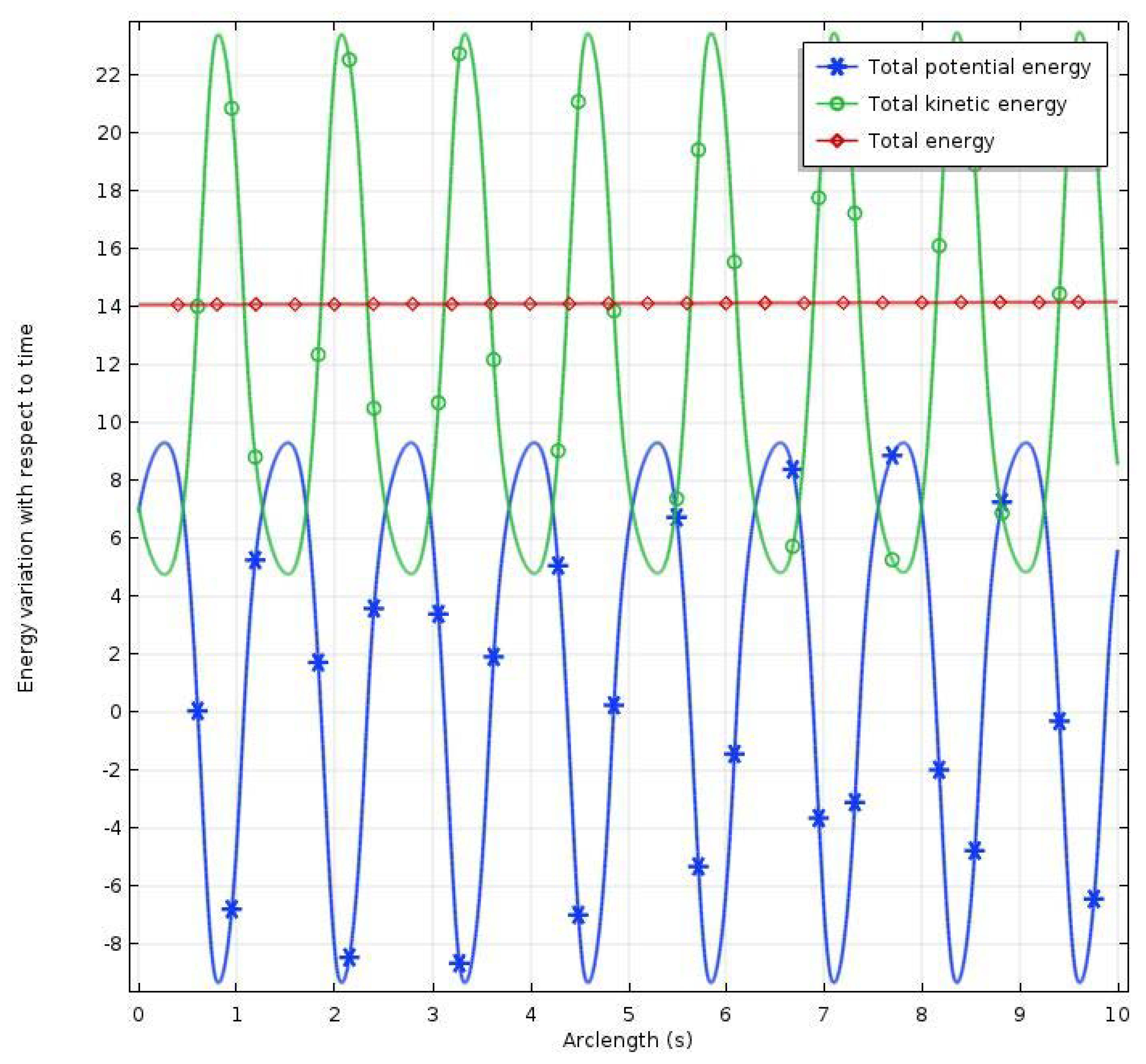
In Figure 1, the energy variation graph of each spherical spacelike magnetic curve for arbitrary value of the geodesic curvature and ${\varpi }_i=1;2;3$ in a time is illustrated.

Although this calculation seems to contain abstract mathematical computation, it turns out to be very valuable to compute since it tells us significant facts about the state of system. For example, Euler–Lagrange equations determine the dynamics of a system considering its simple motion once one computes the energy of the given system. For a given vector field, the following formula is used to describe bending energy of elastica which is a variational problem proposed firstly by Daniel Bernoulli to Leonard Euler in 1744.

$$\mathcal{H}=\frac{1}{2}\int {∥{\nabla }_{{\mathbf{\alpha }}^{\prime }}\mathbf{t}∥}^{2}ds,$$

(16)

where s is an arclength [20]. Once the elastic features of spacelike Sabban magnetic curves are determined, we can state the energy of each spacelike Sabban magnetic curve in terms of the bending energy functional. However, this is the topic of another research that we plan to handle later.

At the beginning of the section, we assert that magnetic curves have a constant energy. Now, we give the constant energy condition that has to be satisfied for each spacelike Sabban magnetic curve in terms of its geodesic curvature.

⧫ Constant energy condition of the $\mathcal{S}\mathit{\alpha }$-magnetic curve in the magnetic vector field $\mathcal{F}$ on the ${\mathcal{S}}_1^2;$

$$-1={(\mu +{\varpi }_1)}^2+{\left({\varpi }_1^{\prime }\right)}^2.$$

Therefore, $\mathcal{S}\mathit{\alpha }$-magnetic curve have no constant energy.

⧫ Constant energy condition of the $\mathcal{S}\mathbf{t}$-magnetic curve in the magnetic vector field $\mathcal{F}$ on the ${\mathcal{S}}_1^2;$

$$-1={({\mu }^{\prime }+{\varpi }_2)}^2+{\left({\varpi }_2^{\prime }\right)}^2-{\left({\varpi }_2\mu \right)}^2.$$

⧫ Constant energy condition of the $\mathcal{S}\mathbf{n}$-magnetic curve in the magnetic vector field $\mathcal{F}$ on the ${\mathcal{S}}_1^2;$

$$-1={\left({\mu }^{\prime }\right)}^2+{(-{\mu }^{\prime }+{\varpi }_3{\mu }^{\prime })}^2-{\left({\varpi }_3^{\prime }\right)}^2.$$

5. Magnetic Force on Spacelike Sabban Magnetic Curves on the ${\mathcal{S}}_{\mathbf{1}}^{\mathbf{2}}$

The Lorentz force equation of the charged particle is described by

$$m\mathbf{a}=\mathbf{F}=q(\mathcal{E}+\mathbf{v}\times \mathcal{F}),$$

where $\mathbf{v}$ is a velocity, m is a mass, q is an electric charge, $\mathcal{F}$ is a magnetic field and $\mathcal{E}$ is an electric field.

The Landau–Hall problem deals with the motion of a charged particle in the presence of a static and constant magnetic field on a Riemannian or a semi-Riemannian surface. If the Lorentz force equation is free of an electric field, then one has

$$m\mathbf{a}=\mathbf{F}=q(\mathbf{v}\times \mathcal{F}).$$

Assuming that there exists a moving charged particle in the magnetic field $\mathcal{B}$, then one has from Equation $\left(4\right)$ and the above identity

$$m\left(-\mathbf{\alpha }-\mu \mathbf{n}\right)=q(\mathbf{v}\times \mathcal{F}).$$

(17)

This statement is important to describe the motion of a charged particle experiencing the Lorentz force.

Furthermore, one is able to induce the charge to mass ratio of the moving charged particle provided that the magnetic field is known. The ratio of the charge to mass is intensely used in the electrodynamics of the charged particles particularly in electron optics, cathode ray tubes, electron microscopy, accelerator and nuclear physics, and mass spectrometry. The significance of the ratio of charge to mass regarding electrodynamics is released on the fact that two particles having the same ratio move in the same trajectory in a vacuum when they are subjected to magnetic fields.

It is also known that magnetic force causes centripetal force, thus cyclotron radius or gyroradius r is described by radius of the curvature of the trajectory of the unit speed magnetic curve whose charge is $q,$ mass is $m,$ speed is $v,$ and strength of the magnetic field is G as the following equality.

$$r=\frac{mv}{qG}.$$

(18)

Theorem 3.

Let β be a moving charged particle such that it corresponds to a unit speed spacelike Sabban magnetic curves in the associated magnetic field $\mathcal{F}$ on the ${\mathcal{S}}_1^2$.

$\mathbf{i}.$ In the case of a $\mathcal{S}\mathit{\alpha }$-magnetic curve$,$ the ratio of charge to mass is $-1,$ the radius of gyration is

$$r=-\frac{1}{{({\mu }^2-1)}^{\frac{1}{2}}},$$

and the gyro-frequency is

$$\varphi =-{({\mu }^2-1)}^{\frac{1}{2}},$$

where ${\varpi }_1=g\left(\varphi \left(\mathbf{n}\right),\mathbf{t}\right)=-\mu$ along with the curve.

$\mathbf{ii}.$ In the case of a $\mathcal{S}\mathbf{t}$-magnetic curve$,$ the ratio of charge to mass is −$1,$ the radius of gyration is

$$r=-\frac{1}{{({\mu }^2+{\varpi }_2^2-1)}^{\frac{1}{2}}},$$

and the gyro-frequency is

$$\psi =-{({\mu }^2+{\varpi }_2^2-1)}^{\frac{1}{2}},$$

where ${\varpi }_2=-g\left(\varphi \left(\mathit{\alpha }\right),\mathbf{n}\right)$ along with the curve.

$\mathbf{iii}.$ In the case of a $\mathcal{S}\mathbf{n}$-magnetic curve, the ratio of charge to mass is −$1,$ the radius of gyration is

$$r=-\frac{1}{{({\mu }^2-1)}^{\frac{1}{2}}},$$

and the gyro-frequency is

$$\varphi =-{({\mu }^2-1)}^{\frac{1}{2}},$$

where ${\varpi }_3=g\left(\varphi \left(\mathit{\alpha }\right),\mathbf{t}\right)=1$ along with the curve.

Proof. 

Let $\alpha$ be a $\mathcal{S}\mathit{\alpha }$-magnetic curve of the magnetic field $\mathcal{F}$ on the ${\mathcal{S}}_1^2.$ One already knows from the Equations (7) and (8)

$$\mathcal{F}={\varpi }_1\mathbf{\alpha }-\mathbf{n}.$$

If we also consider the Lorentz force equation given by Equation (17), then it gives

$$\frac{q}{m}=-1and{\varpi }_1=-\mu .$$

The magnitude of the given magnetic field is

$$\mathcal{F}={({\mu }^2-1)}^{\frac{1}{2}}.$$

 ☐

Now, if one takes into account Equation (18) and the above equalities, then it is easy to reach the result. The rest of the proof is completed if one follows similar steps for the other cases.

In Figure 2a, the magnetic trajectories of the $\mathcal{S}\mathit{\alpha }$-magnetic curve and $\mathcal{S}\mathbf{n}$-magnetic curve are drawn by considering the gyration radius of the curve.

In Figure 2b, a different demonstration is used to observe the $\mathcal{S}\mathbf{t}$-magnetic curve by considering the gyration radius of the curve.

6. Uniform Motion of Spacelike Sabban Magnetic Curves on the ${\mathcal{S}}_{\mathbf{1}}^{\mathbf{2}}$

The description of a uniformly accelerated motion (UAM) in relativity has always been of great interest for many scientists. For example, Rindler used the relation between Lorentzian circles and uniformly accelerated motion in Minkowski spacetime to determine hyperbolic motion in General Relativity [21,22]. Covariant definition of the UAM and its explicit solutions were investigated by Friedman and Scarr [23,24]. The notion of the UAM was analyzed in detail by giving its novel geometric characterization by Fuente and Romero [25]. The description of the unchanged direction motion (UDM) was presented by extending the UAM by Fuente, Romero, and Torres [26]. The intrinsic definition of the uniformly circular motion (UCM) was given by Fuente, Romero, and Torres as a particular case of a planar motion [27]. In this section, we investigate the UAM, UDM, and UCM of the moving charged particle corresponding to any unit speed spacelike Sabban magnetic curve in the associated magnetic field $\mathcal{F}$ on the ${\mathcal{S}}_1^2.$ We determine necessary and sufficient conditions that have to be satisfied by the particle in terms of the Sabban scalars of the worldline of magnetic curves. We use following definitions of the UAM, UDM, and UCM.

Definition 4.

The particle obeys a UAM if

$${\nabla }_{FW}\left({\nabla }_{{\mathbf{\alpha }}^{\prime }}{\mathbf{\alpha }}^{\prime }\right)=0,$$

(19)

where ${\nabla }_{FW}$ is a Fermi–Walker derivative connection of the curve $\mathit{\alpha }$ [25].

Definition 5.

The particle obeys a UDM if

$${\left|{\nabla }_{{\mathbf{\alpha }}^{\prime }}{\mathbf{\alpha }}^{\prime }\right|}^2=\mathit{constant},$$

(20)

and

$${\left|{\nabla }_{FW}\left({\nabla }_{{\mathbf{\alpha }}^{\prime }}{\mathbf{\alpha }}^{\prime }\right)\right|}^2=\mathit{constant},$$

(21)

ç where ${\nabla }_{FW}$ is a Fermi–Walker derivative connection of the curve $\mathit{\alpha }$ [26].

Definition 6.

The particle obeys a UCM if

$${\nabla }_{FW}\left({\left|{\nabla }_{{\mathbf{\alpha }}^{\prime }}{\mathbf{\alpha }}^{\prime }\right|}^{-1}{\nabla }_{{\alpha }^{\prime }}{\mathbf{\alpha }}^{\prime }\right)=0,$$

(22)

where ${\nabla }_{FW}$ is a Fermi–Walker derivative connection of the curve $\mathit{\alpha }$ [27].

Definition 7.

Let ${\nabla }_{FW}$ be the covariant derivative corresponding to Levi–Civita connection ∇ of h. Then, we have [28].

$${\nabla }_{FW}\mathcal{R}={\nabla }_{{\mathbf{\alpha }}^{\prime }}\mathcal{R}-g\left({\alpha }^{\prime },\mathcal{R}\right){\nabla }_{{\mathbf{\alpha }}^{\prime }}{\mathbf{\alpha }}^{\prime }+g({\nabla }_{{\mathbf{\alpha }}^{\prime }}{\mathbf{\alpha }}^{\prime },\mathcal{R}){\mathbf{\alpha }}^{\prime },$$

(23)

where $\mathcal{R}$ is any vector field along the curve $\mathit{\alpha }.$

In the presence of an electromagnetic field, dynamics of the charged particle is defined by the Lorentz force [26,29,30,31,32,33,34]. Now, let $\beta$ be a moving charged particle such that it corresponds to a unit speed spacelike Sabban magnetic curves in the associated magnetic field $\mathcal{F}$ on the ${\mathcal{S}}_1^2$.

⧫ In the case of a $\mathcal{S}\mathit{\alpha }$-magnetic curve, the magnetic trajectories obey the UAM iff

$${\nabla }_{FW}\left(\varphi \left(\mathbf{\alpha }\right)\right)=0.$$

(24)

the magnetic trajectories obey the UDM iff

$${\left|\varphi \left(\mathbf{\alpha }\right)\right|}^2,{\left|{\nabla }_{FW}\left(\varphi \left(\mathbf{\alpha }\right)\right)\right|}^2$$

(25)

are both constant; and the magnetic trajectories obey the UCM iff

$${\nabla }_{FW}({\left|\varphi \left(\mathbf{\alpha }\right)\right|}^{-1}\varphi \left(\mathbf{\alpha }\right))=0.$$

(26)

Corollary 1.

$\mathbf{i}.$ If one considers Equations (6), (23) and (24), then it is computed that

$${\nabla }_{FW}\left(\varphi \left(\mathbf{\alpha }\right)\right)=0.$$

Thus, the magnetic trajectories of the $\mathcal{S}\mathit{\alpha }$-magnetic curve obey the UAM.

$\mathbf{ii}.$ If one considers Equations (6), (23) and (25), then it is computed that

$${\left|\varphi \left(\mathbf{\alpha }\right)\right|}^2=1\mathrm{and}{\left|{\nabla }_{FW}\left(\varphi \left(\mathbf{\alpha }\right)\right)\right|}^2=0.$$

Thus, the magnetic trajectories of the $\mathcal{S}\mathit{\alpha }$-magnetic curve obey the UDM.

$\mathbf{iii}.$ If one considers Equations (6), (23) and (26), then it is computed that

$${\nabla }_{FW}({\left|\varphi \left(\mathbf{\alpha }\right)\right|}^{-1}\varphi \left(\mathbf{\alpha }\right))=0.$$

Thus, the magnetic trajectories of the $\mathcal{S}\mathit{\alpha }$-magnetic curve obey the UCM.

In Figure 3, the magnetic trajectories of the $\mathcal{S}\mathit{\alpha }$-magnetic curvem which is proved to obey the UAM, UDM, and UCM, on the section of the pseudo-three-sphere, are shown.

⧫ In the case of a $\mathcal{S}\mathbf{t}$-magnetic curve$,$ the magnetic trajectories obey the UAM iff

$${\nabla }_{FW}\left(\varphi \left(\mathbf{t}\right)\right)=0.$$

(27)

the magnetic trajectories obey the UDM iff

$${\left|\varphi \left(\mathbf{t}\right)\right|}^2,{\left|{\nabla }_{FW}\left(\varphi \left(\mathbf{t}\right)\right)\right|}^2,$$

(28)

are both constant; and the magnetic trajectories obey the UCM iff

$${\nabla }_{FW}({\left|\varphi \left(\mathbf{t}\right)\right|}^{-1}\varphi \left(\mathbf{t}\right))=0.$$

(29)

Corollary 2.

$\mathbf{i}.$ If one considers Equations (6), (23) and (27), then it is computed that

$${\nabla }_{FW}\left(\varphi \left(\mathbf{t}\right)\right)=-{\mu }^{\prime }\mathbf{n}.$$

Thus, the magnetic trajectories of the $\mathcal{S}\mathbf{t}$-magnetic curve obey the UAM iff the geodesic curvature is a constant, i.e., trajectories follow a pseudo-circle whose center Ω lies on the ${\mathcal{S}}_1^2$. Here, the center is defined by

$$\mathsf{\Omega }=\left(\mu \mathbf{\alpha }-\mathbf{n}\right)/{\left(1+{\mu }^2\right)}^{\frac{1}{2}}.$$

Here, one can check Ref. [18] to see the computation of the center of the pseudo-circle on ${\mathcal{S}}_1^2.$

$\mathbf{ii}.$ If one considers Equations (6), (23) and (28), then it is computed that

$${\left|\varphi \left(\mathbf{t}\right)\right|}^2=1-{\mu }^{2}and{\left|{\nabla }_{FW}\left(\varphi \left(\mathbf{t}\right)\right)\right|}^2=-{\left({\mu }^{\prime }\right)}^2.$$

Thus, the magnetic trajectories of the $\mathcal{S}\mathbf{t}$-magnetic curve obey the UDM iff the geodesic curvature is a constant, i.e., trajectories follow a pseudo-circle whose center Ω lies on the ${\mathcal{S}}_1^2.$

$\mathbf{iii}.$ If one considers Equations (6), (23) and (29), then it is computed that

$${\nabla }_{FW}({\left|\varphi \left(\mathbf{t}\right)\right|}^{-1}\varphi \left(\mathbf{t}\right))=[-\frac{{\lambda }^{\prime }}{{\lambda }^2}(-1+{\mu }^2)+\mu {\mu }^{\prime }+\lambda {\mu }^2]\mathbf{t}+[\frac{{\lambda }^{\prime }}{{\lambda }^2}{\mu }^{\prime }-\lambda {\mu }^{″}]\mathbf{n},$$

where $\lambda ={[{(-1+{\mu }^2)}^2-{\left({\mu }^{\prime }\right)}^2]}^{-1/2}.$ Thus, the magnetic trajectories of the $\mathcal{S}\mathbf{t}$-magnetic curve obey the UCM iff

$$\begin{array}{ccc}\hfill \mu {\mu }^{\prime }+\lambda {\mu }^2& =& \frac{{\lambda }^{\prime }}{{\lambda }^2}(-1+{\mu }^2),\hfill \\ \hfill \frac{{\lambda }^{\prime }}{{\lambda }^2}{\mu }^{\prime }& =& \lambda {\mu }^{″}.\hfill \end{array}$$

Figure 4 shows a sample of the magnetic trajectories of the $\mathcal{S}\mathbf{t}$-magnetic curve, which are proved to obey the UAM, UDM, and UCM, at the section of the pseudo-three-sphere for given arbitrary centers of pseudo-circles on $S_1^2.$

⧫ In the case of a $\mathcal{S}\mathbf{n}$-magnetic curve, the magnetic trajectories obey the UAM iff

$${\nabla }_{FW}\left(\varphi \left(\mathbf{n}\right)\right)=0.$$

(30)

the magnetic trajectories obey the UDM iff

$${\left|\varphi \left(\mathbf{n}\right)\right|}^2,{\left|{\nabla }_{FW}\left(\varphi \left(\mathbf{n}\right)\right)\right|}^2,$$

(31)

are both constant; and the magnetic trajectories obey the UCM iff

$${\nabla }_{FW}({\left|\varphi \left(\mathbf{n}\right)\right|}^{-1}\varphi \left(\mathbf{n}\right))=0.$$

(32)

Corollary 3.

$\mathbf{i}.$ If one considers Equations (6), (23) and (30), then it is computed that

$${\nabla }_{FW}(\varphi \left(\mathbf{n}\right)=-\mu \mathbf{t}.$$

Thus, the magnetic trajectories of the $\mathcal{S}\mathbf{n}$-magnetic curve obey the UAM iff the geodesic curvature is a constant i.e., trajectories follow a pseudo-circle whose center Ω lies on the ${\mathcal{S}}_1^2$. Here, the center is defined by $\mathsf{\Omega }=\left(\mu \mathit{\alpha }-\mathbf{n}\right)/{\left(1+{\mu }^2\right)}^{\frac{1}{2}}$ [18].

$\mathbf{ii}.$ If one considers Equations (6), (23) and (31), then it is computed that

$${\left|\varphi \left(\mathbf{n}\right)\right|}^2={\mu }^2\mathrm{and}{\left|{\nabla }_{FW}\left(\varphi \left(\mathbf{n}\right)\right)\right|}^2={\left({\mu }^{\prime }\right)}^2.$$

Thus, the magnetic trajectories of the $\mathcal{S}\mathbf{n}$-magnetic curve obey the UDM iff the geodesic curvature is a constant, i.e., trajectories follow a pseudo-circle whose center Ω lies on the ${\mathcal{S}}_1^2.$

$\mathbf{iii}.$ If one considers Equations (6), (23) and (32), then it is computed that

$${\nabla }_{FW}\left({\left|\varphi \left(\mathbf{n}\right)\right|}^{-1}\varphi \left(\mathbf{n}\right)\right)=0.$$

Thus, the magnetic trajectories of the $\mathcal{S}\mathbf{n}$-magnetic curve obey the UCM.

Figure 5 shows the magnetic trajectories of the $Sn$-magnetic curve, which is proved to obey the UAM, UDM, and UCM, at the section of the pseudo-three-sphere. Here, the center of the pseudo-circle for the case of UAM and UDM is also computed.

7. Conclusions

Sideway force is experienced by the charged particle whose motion is determined by the trajectory of the curve in the magnetic field. It is proportional to the component of the velocity, the strength of the magnetic field, and the charge of the particle. This is the Lorentz force and it is stated by

$$\varphi \left(\mathcal{A}\right)=\mathcal{F}\times \mathcal{A}.$$

This paper presents new type of spacelike magnetic curves associated with the Sabban vector field defined in the Minkowski space. In this approach, the necessary and sufficient conditions of the uniformity of the spatial magnetic curves aee analyzed lying on the ${\mathbb{S}}_1^2$. In light of these results, we will study this concept on the Hyperbolic space.

References

- Bacry, H.; Levy-Leblond, J.M. Possible Kinematics. J. Math. Phys. 1968, 9, 1605. [Google Scholar] [CrossRef]
- Baş, S.; Körpınar, T. A New Characterization of One Parameter Family of Surfaces by Inextensible Flows in De-Sitter 3-Space. J. Adv. Phys. 2018, 7, 251–256. [Google Scholar] [CrossRef]
- Fusho, T.; Izumiya, S. Lightlike surfaces of spacelike curves in de Sitter 3-space. J. Geom. 2009, 88, 19–29. [Google Scholar] [CrossRef]
- Huang, C.G.; Guo, H.Y.; Tian, Y.; Xu, Z.; Zhou, B. Newton-Hooke Limit of Beltrami-de Sitter Spacetime. Mod. Phys. Lett. A 2004, 19, 2535–2562. [Google Scholar]
- Barros, M.; Romero, A.; Cabrerizo, J.L.; Fernández, M. The Gauss–Landau–Hall problem on Riemannian surfaces. J. Math. Phys. 2005, 46. [Google Scholar] [CrossRef]
- Sunada, T. Magnetic flows on a Riemann surface. In Proceedings of the KAIST Mathematics Workshop: Analysis and Geometry, Taejeon, Korea, 3–6 August 1993; KAIST: Daejeon, Korea, 1993. [Google Scholar]
- Druta-Romaniuc, S.L.; Munteanu, M.I. Magnetic Curves corresponding to Killing magnetic fields in . J. Math. Phys. 2011, 52, 113506. [Google Scholar] [CrossRef]
- Druţă-Romaniuc, S.L.; Munteanu, M.I. Killing magnetic curves in a Minkowski3-space. Nonlinear Anal. Real World Appl. 2013, 14, 383–396. [Google Scholar] [CrossRef]
- Cabrerizo, J.L.; Fernandez, M.; Gomez, J.S. On the existence of almost contact structure and the contact magnetic field. Acta Math. Hungar. 2009, 125, 1–2. [Google Scholar] [CrossRef]
- Korpinar, T.; Demirkol, R.C. Frictional magnetic curves in 3D Riemannian manifolds. Int. J. Geom. Methods Mod. Phys. 2018, 15, 1850020-1. [Google Scholar]
- Körpınar, T. On T-Magnetic Biharmonic Particles with Energy and Angle in the Three Dimensional Heisenberg Group . Adv. Appl. Clifford Algebras 2018, 28, 9. [Google Scholar] [CrossRef]
- Körpınar, T. A New Version of Normal Magnetic Force Particles in 3D Heisenberg Space. Adv. Appl. Clifford Algebras 2018, 28, 83. [Google Scholar] [CrossRef]
- Barros, M.; Cabrerizo, J.L.; Fernandez, M.; Romero, A. Magnetic vortex filament flows. J. Math. Phys. 2007, 48, 082904. [Google Scholar] [CrossRef] [Green Version]
- Cabrerizo, J.L. Magnetic fields in 2D and 3D sphere. J. Nonlinear Math. Phys. 2013, 20, 440–450. [Google Scholar] [CrossRef] [Green Version]
- Bozkurt, Z.; Gök, I.; Yaylı, Y.; Ekmekci, F.N. A new approach for magnetic curves in 3D Riemannian manifolds. J. Math. Phys. 2014, 55, 053501. [Google Scholar] [CrossRef] [Green Version]
- Koenderink, J.J. Solid Shape; MIT Press: Cambridge, MA, USA, 1990. [Google Scholar]
- Izumiya, S.; Nagai, T. Generalized Sabban curves in the Euclidean n -sphere and spherical duality. Res. Math. 2017, 72, 401. [Google Scholar] [CrossRef]
- Babaarslan, M.; Yaylı, Y. On space-like constant slope surfaces and Bertrand curves in Minkowski 3-space. Analele Stiintifice ale Universitatii Al I Cuza din Iasi Matematica 2017, 2, 323. [Google Scholar] [CrossRef]
- Wood, C.M. On the Energy of a Unit Vector Field. Geom. Dedicata 1997, 64, 319–330. [Google Scholar] [CrossRef]
- Guven, J.; Valencia, D.M.; Vazquez-Montejo, J. Environmental bias and elastic curves on surfaces. Phys. A Math. Theory 2014, 47, 355201. [Google Scholar] [CrossRef] [Green Version]
- Rindler, W. Lenght contraction paradox. Am. J. Phys. 1961, 24, 365. [Google Scholar] [CrossRef]
- Rindler, W. Hyperbolic motion in curved space time. Phys. Rev. 1961, 119, 2082–2089. [Google Scholar] [CrossRef]
- Friedman, Y.; Scarr, T. Making the relativistic dynamics equation covariant: Explicit solutions for motion under a constant force. Phys. Scr. 2012, 86, 065008. [Google Scholar] [CrossRef]
- Friedman, Y.; Scarr, T. Uniform acceleration in general relativity. Gen. Relativ. Gravit. 2015, 47, 121. [Google Scholar] [CrossRef]
- De la Fuente, D.; Romero, A. Uniformly accelerated motion in General Relativity: Completeness of inextensible trajectories. Gen. Relativ. Gravit. 2015, 47, 33. [Google Scholar] [CrossRef]
- De la Fuente, D.; Romero, A.; Torres, P.J. Unchanged direction motion in general relativity: The problems of prescribing acceleration and the extensibility of trajectories. J. Math. Phys. 2015, 56, 112501. [Google Scholar] [CrossRef]
- De la Fuente, D.; Romero, A.; Torres, P.J. Uniform circular motion in general relativity: Existence and extendibility of the trajectories. Class. Quantum Gravity 2017, 34, 125016. [Google Scholar] [CrossRef]
- Sachs, R.K.; Wu, H. General Relativity for Mathematicians; Graduate Texts in Mathematics; Springer: New York, NY, USA, 1977; Volume 48. [Google Scholar]
- Körpınar, T.; Demirkol, R.C.; Asil, V. The motion of a relativistic charged particle in a homogeneous electromagnetic field in De-Sitter space. Revista Mexicana de Fisica 2018, 64, 176. [Google Scholar]
- Körpınar, T.; Demirkol, R.C. Energy on a timelike particle in dynamical and electrodynamical force fields in De-Sitter space. Rev. Mex. Fis. 2017, 63, 560–568. [Google Scholar]
- Asil, V.; Körpınar, T.; Baş, S. Inextensible flows of timelike curves with Sabban frame in . Siauliai Math. Semin. 2012, 7, 5–12. [Google Scholar]
- Körpınar, T. On Velocity Magnetic Curves in Terms of Inextensible Flows in Space. J. Adv. Phys. 2018, 7, 257–260. [Google Scholar] [CrossRef]
- Baş, S.; Körpınar, T. Inextensible Flows of Spacelike Curves on Spacelike Surfaces according to Darboux Frame in . Bol. Soc. Paran. Mat. 2013, 31, 9–17. [Google Scholar] [CrossRef]
- Körpınar, T.; Baş, S. On evolute curves in terms of inextensible flows of in . Bol. Soc. Paran. Mat. 2018, 36, 117–124. [Google Scholar] [CrossRef]
Figure 1.
Energy variation graph of each spherical spacelike magnetic curve.
Figure 2.
(a) Gyroradius for a magnetic curve and magnetic curve for certain values in magnetic field; (b) Gyroradius for a magnetic curve for certain values in magnetic field.
Figure 3.
Magnetic trajectories of the -magnetic curve.
Figure 4.
Magnetic trajectories of the t-magnetic curve.
Figure 5.
Magnetic trajectories of the n-magnetic curve.
© 2018 by the author. Licensee MDPI, Basel, Switzerland. This article is an open access article distributed under the terms and conditions of the Creative Commons Attribution (CC BY) license (http://creativecommons.org/licenses/by/4.0/).
Share and Cite
MDPI and ACS Style