New Methodology to Approximate Type-Reduction Based on a Continuous Root-Finding Karnik Mendel Algorithm


Tijuana Institute of Technology, 22414 Tijuana, Mexico
*
Author to whom correspondence should be addressed.
Algorithms 2017, 10(3), 77; https://doi.org/10.3390/a10030077
Submission received: 30 May 2017
/
Revised: 29 June 2017
/
Accepted: 1 July 2017
/
Published: 5 July 2017
(This article belongs to the Special Issue Extensions to Type-1 Fuzzy Logic: Theory, Algorithms and Applications)
Abstract
:Interval Type-2 fuzzy systems allow the possibility of considering uncertainty in models based on fuzzy systems, and enable an increase of robustness in solutions to applications, but also increase the complexity of the fuzzy system design. Several attempts have been previously proposed to reduce the computational cost of the type-reduction stage, as this process requires a lot of computing time because it is basically a numerical approximation based on sampling, and the computational cost is proportional to the number of samples, but also the error is inversely proportional to the number of samples. Several works have focused on reducing the computational cost of type-reduction by developing strategies to reduce the number of operations. The first type-reduction method was proposed by Karnik and Mendel (KM), and then was followed by its enhanced version called EKM. Then continuous versions were called CKM and CEKM, and there were variations of this and also other types of variations that eliminate the type-reduction process reducing the computational cost to a Type-1 defuzzification, such as the Nie-Tan versions and similar enhancements. In this work we analyzed and proposed a variant of CEKM by viewing this process as solving a root-finding problem, in this way taking advantage of existing numerical methods to solve the type-reduction problem, the main objective being eliminating the type-reduction process and also providing a continuous solution of the defuzzification.
1. Introduction
Nowadays, Type-1 and Type-2 fuzzy logic have demonstrated many advantages with respect to classical modeling methods, for example, their robustness, and design without a plant mathematical model. These advantages allow a relatively easy implementation in specific applications, for example, [1,2] provide a review of control applications, [3] is an overview of pattern recognition and classification, [4,5,6] details hardware implementations of fuzzy systems, image processing [7], and many other applications as mentioned in [8]. However, the implementation of these algorithms usually requires a higher computational cost with respect to their classical counter parts.
The computational cost of Interval Type-2 fuzzy logic was increased with respect to Type-1 fuzzy logic, of course achieving better results, but at the expense of having a higher computational cost. The implementation of Interval Type-2 fuzzy inference systems (FISs) requires around double the computational cost than Type-1 fuzzy inference systems, but could be even higher because the complexity of the centroid calculation increases in IT2 FISs, and the process to obtain the centroid of IT2 FIS is called type-reduction [9].
The original type-reduction method was proposed by Karnik and Mendel in [10] and was called the Karnik-Mendel Algorithm (KM), and based on this method many variations have emerged, like the Enhanced Karnik-Mendel (EKM) [11], Continuous Karnik-Mendel (CKM), and Continuous Enhanced Karnik-Mendel (CEKM). These variations of the KM type reductions were proposed in order to reduce the type-reduction computational cost; and this is because in an IT2 FIS the process that requires the highest computational cost is in fact the type reduction.
The goal of decreasing the type-reduction computational cost have been considered by several researchers, for example, in [12] the need for sorting is eliminated, in [13] a linear approximation of KM type reduction was realized, in [14] a polynomial regression for type reduction is realized, [15] introduces the Nie-Tan type reduction as an alternative to reduce the computational cost of this process by eliminating the type-reduction process, and [16] provides an study of several type-reduction alternatives focused on computational cost reduction.
The contribution of the present work is a proposed new CEKM type-reduction approximation and also providing a methodology for its implementation. This method is based on CEKM as root-finding problem, which was proposed by Liu and Mendel in [17]. This method for type reduction is based on two proposed equations that allow approximation of the output points through numerical methods, like Newton Raphson [18]. The objective is to provide a solution of type-reduction/defuzzification problem that eliminates the iterations and sampling requirements. In addition, we compare this approximation method with respect to the classical type-reductions approaches and propose in which context is recommendable to use our approach.
The organization of the present work is as follows: Section 2 introduces the concepts of Interval Type-2 fuzzy inference systems, then Section 3 is focused on the type-reduction process, Section 4 presents the fundamentals of the proposed approximation of type reduction, Section 5 introduces the proposed methodology to realize the type-reduction approximation, Section 6 and Section 7 outline two applications of our proposed methodology and their corresponding results, and finally Section 8 contains the conclusion and future work.
2. Interval Type 2 Fuzzy Inference Systems
Type-1 fuzzy logic was proposed as a vagueness model of human language [19], by considering continuous membership degrees between 0 and 1 related with concepts or attributes in order to make decisions. Now, the emergence of Interval Type-2 fuzzy logic provides not only a vagueness model but also an uncertainty model [20,21], in this way increasing the systems’ robustness and improving their performance.
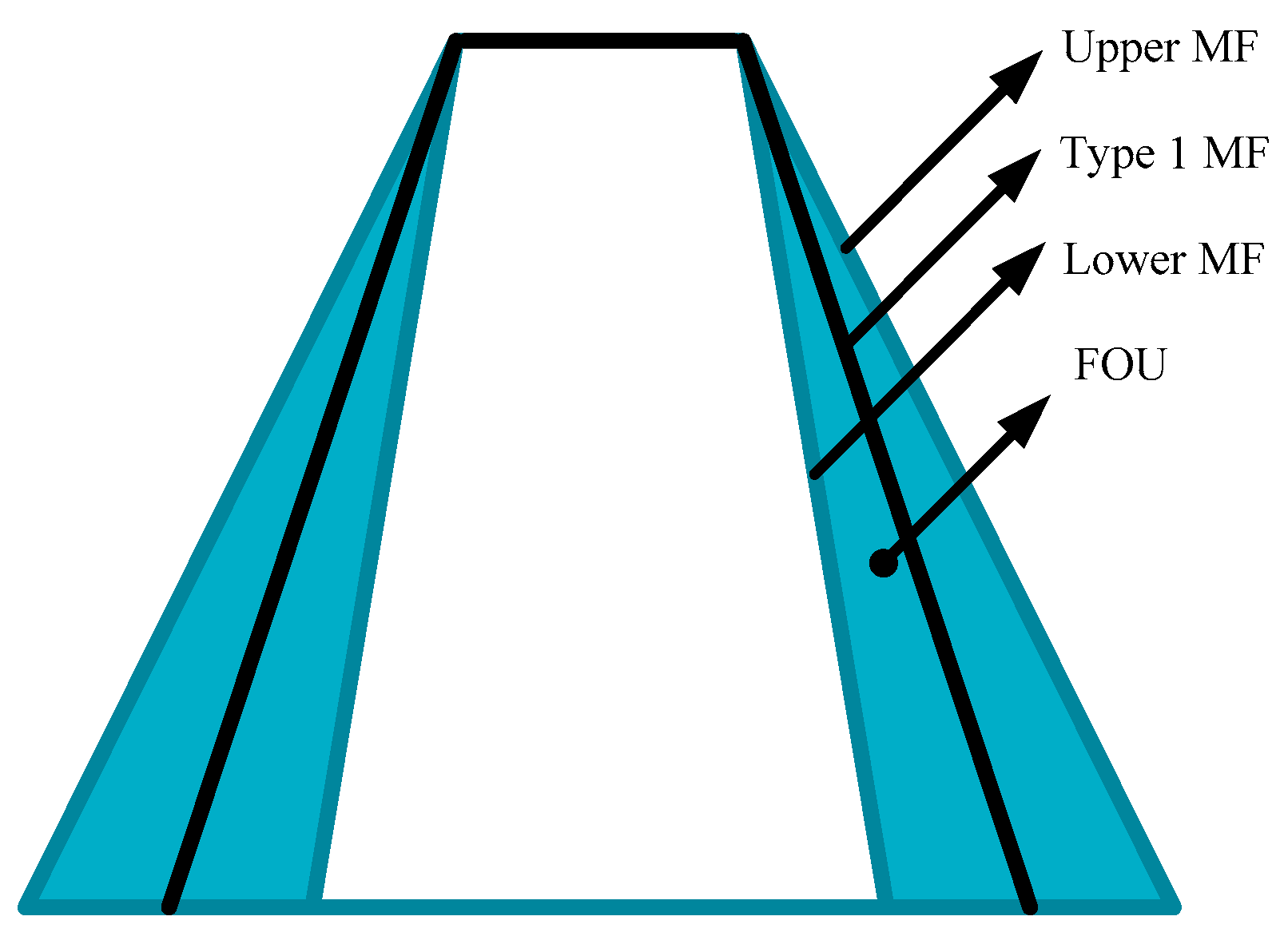
Interval Type-2 fuzzy membership functions are defined by two Type-1 membership functions, called upper membership function and lower membership function, and the area between these membership functions is called the footprint of uncertainty. A graphical illustration of these concepts can be appreciated in Figure 1 and it is mathematically defined in Equation (1).
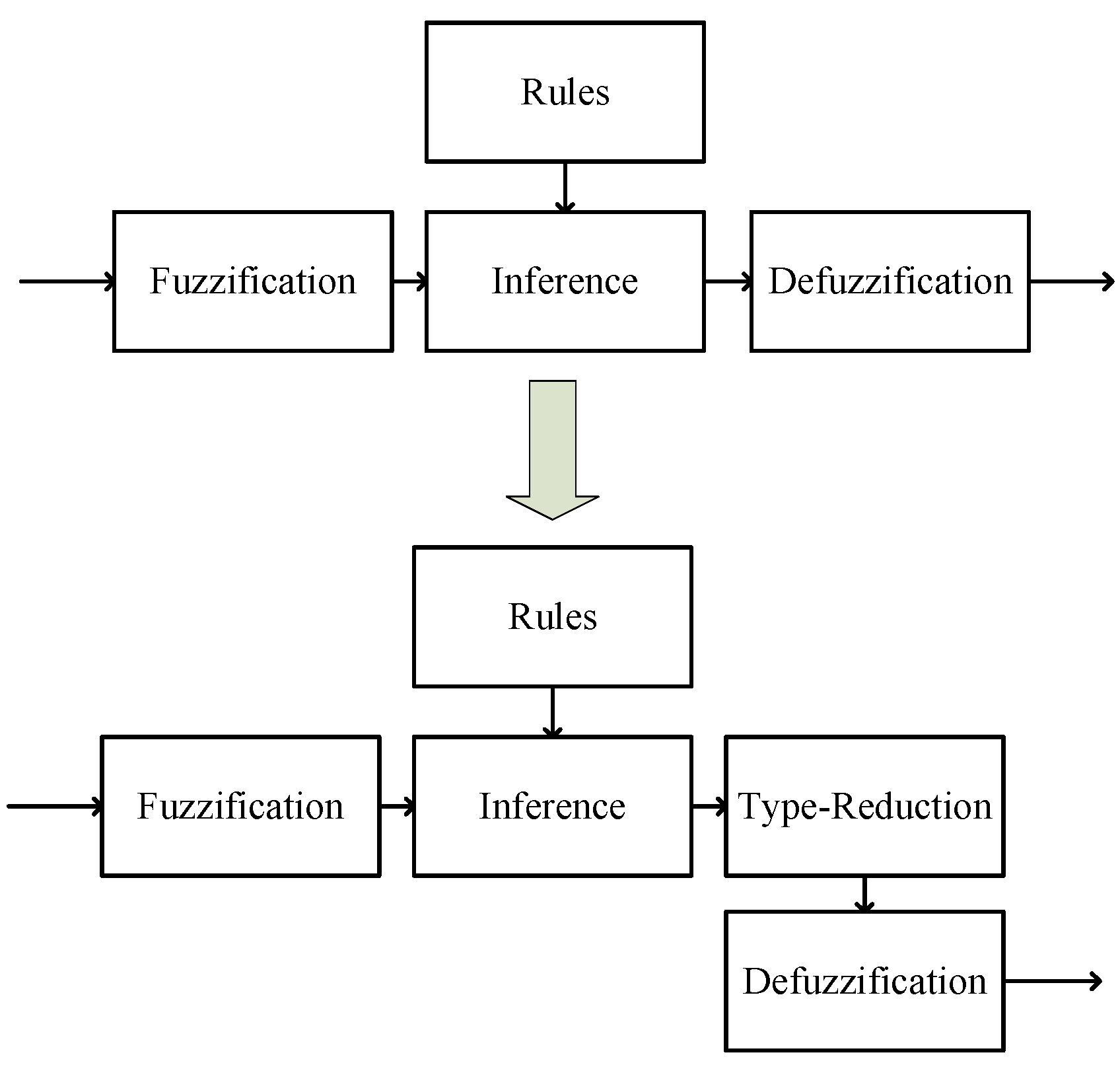
The implementation of Interval Type-2 fuzzy logic concepts require also to extend the special T-norm and S-norm operations to the join and meet operations [22], and the fuzzy inference system is modified as illustrated in Figure 2.
The main difference resides in the defuzzification; this process is very interesting because in Type-1 fuzzy inference systems it is realized by the centroid method, but in an IT2 FIS the process for defuzzification is realized by a new process called type-reduction. This process is significantly more complex than defuzzification and is explained in Section 3.
3. Type-Reduction Algorithms
Currently, there exist different algorithms in order to obtain the centroid of the IT2 MFs [9], and the most-used type-reduction methods are inspired in the Karnik Mendel algorithm. This algorithm is summarized in Table 1.
The main goal of this algorithm is to find the critical points that define the combination of upper and lower membership functions, and these points are called the switch points.
4. Continuous Karnik-Mendel Algorithm as a Root-Finding Problem
In [17] a CKM that extends the KM type-reduction algorithm in a continuous form, as shown Equations (2) and (3), is presented.
Starting with Equations (2) and (3) is possible to express the type-reduction process as a root-finding problem [18]. In this regard, Liu and Mendel proposed Equations (4) and (5).
Thanks to this proposal it is possible to use root-finding numerical methods, for example Newton-Raphson, and now the problem can be expressed as follows (Equations (6) and (7)).
However, the mathematical development for obtaining an analytical solution still represents a challenge for the implementation. This is because in real applications, the upper and lower membership functions for type-reduction are composed functions, which results on an inference system with many factors that add complexity to the functions.
5. Proposed CEKM Approximation and Methodology
In order to reduce the type-reduction computational cost, we propose a methodology for type-reduction approximation. First, we propose that the first iteration of the Newton Raphson method, expressed in Equations (6) and (7), is a good enough type-reduction approximation and this can be expressed in Equations (8) and (9).
where and respectively are based on the EKM initialization explained by Liu et al. in [23], and these are expressed in Equation (10).
This type-reduction approximation proposed in Equations (14) and (15) shows several advantages with respect to classical type reduction, such as KM or EKM, and some examples of these advantages is that the approximation does not require discretization, and this is because it is an analytical solution, another advantage is that it is easy to implement in limited platforms, for example, in hardware applications.
However, this approximation is not possible without a mathematical definition of the and functions, and these functions are defined by intervals. The mathematical approach for the and functions is very complex because they depend on the composition operation for all consequent membership functions and rule-firing forces.
In order to outline a methodology, a mathematical development is presented that allows describing Equations (4) and (5) by using intervals.
Considering Equations (11) and (12) based on the concept of integration by parts
To simplify, we propose the A and V upper and lower functions that compose the and functions expressed in Equations (11) and (12). The functions A and V are expressed in Equation (13).
Now, based on the A and V functions, Equation (14) express the and functions.
where and are the initial switch points, computed with Equation (10), and is necessary to identify the intervals where there points are located, and these are denoted in Equation (14) as , , , and .
Now, based on Equation (14), we propose a methodology to obtain the functions by intervals and finally be able to use Equations (8) and (9) to obtain the analytical CEKM approximation. This methodology is summarized in Table 2.
Following this proposed methodology, the final results are two equations in function of the firing force and the initial centroids, remembering that these initial centroids are static and are computed by the CEKM criteria.
The resultant equations are non-iterative and do not depend on sampling, and this is the reason of the computational cost reduction.
• Implementation restrictions.
The approximate CEKM implementation success depends on the mathematical approach to Equations (11) and (12), remembering that in an FIS, these equations will be dynamic by the variation of the system inputs.
To obtain Equations (11) and (12) it is necessary before to obtain the fuzzy set B, expressed in Equation (15), and this fuzzy set is the result of the composition operation. This means the implication of each rule-firing force with their respective output fuzzy set (Equation (16)), and the aggregation of all implications (Equation (16)).
where represents the rule firing force, represents the membership degree with respect to the corresponding output fuzzy set, and the implication is realized by the T-norm operation.
On the other hand, the aggregation is realized by the S-Norm operation.
The selection of the operations for implication and aggregation is very important; the most-used composition is the Mamdani implication, Max as the S-Norm, and Min as the T-Norm.
We propose to use the probor-prod composition, and this is because it is necessary to mathematically define these operations.
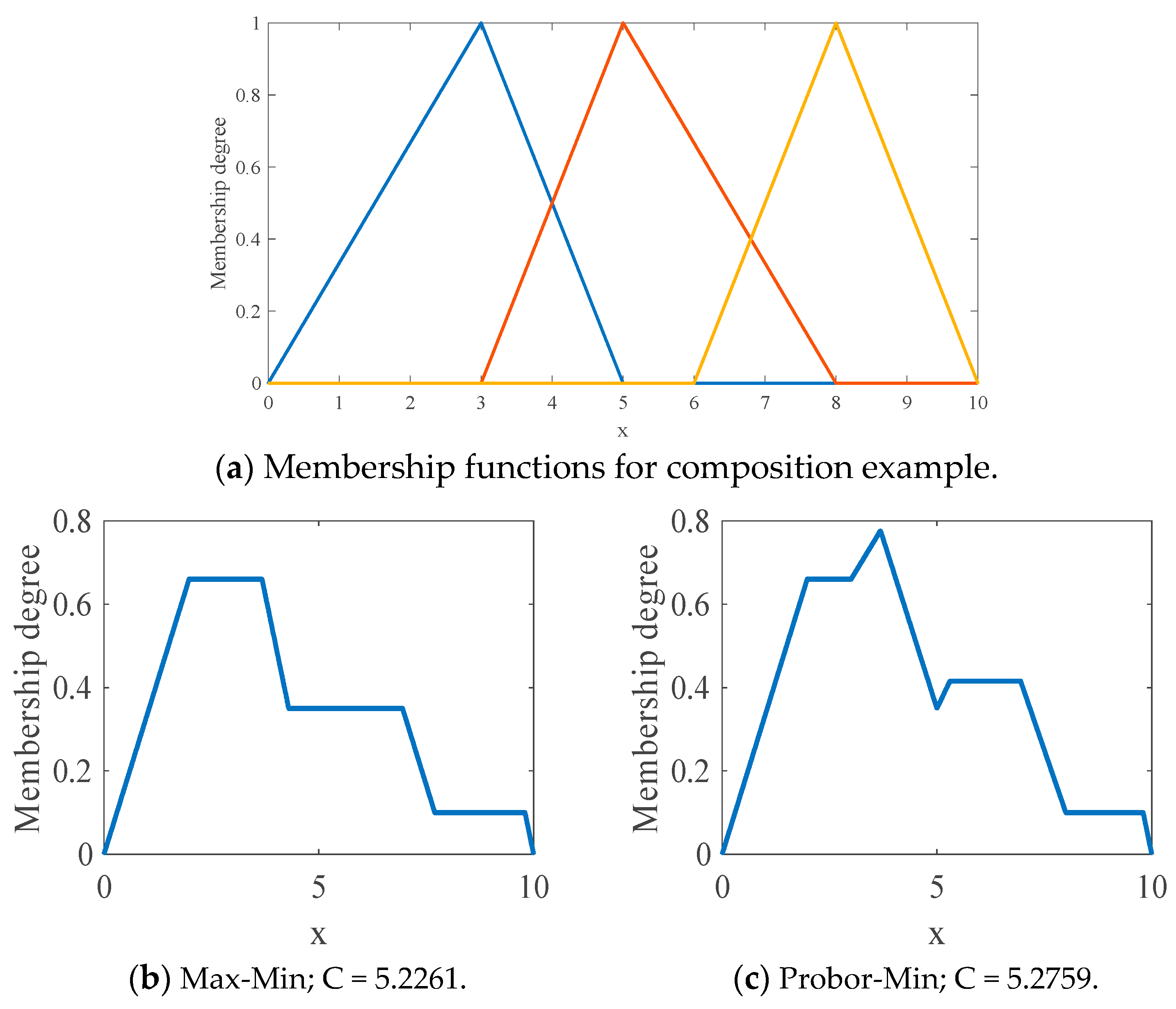
Figure 3 shows four different composition operations and their corresponding centroids. This Type-1 MF used for this example has three Triangular MFs. The centroids of these composition alternatives are a slightly different; however, the restriction on the proposed methodology is the use of the Probor-Prod composition, because this composition is mathematically more approachable.
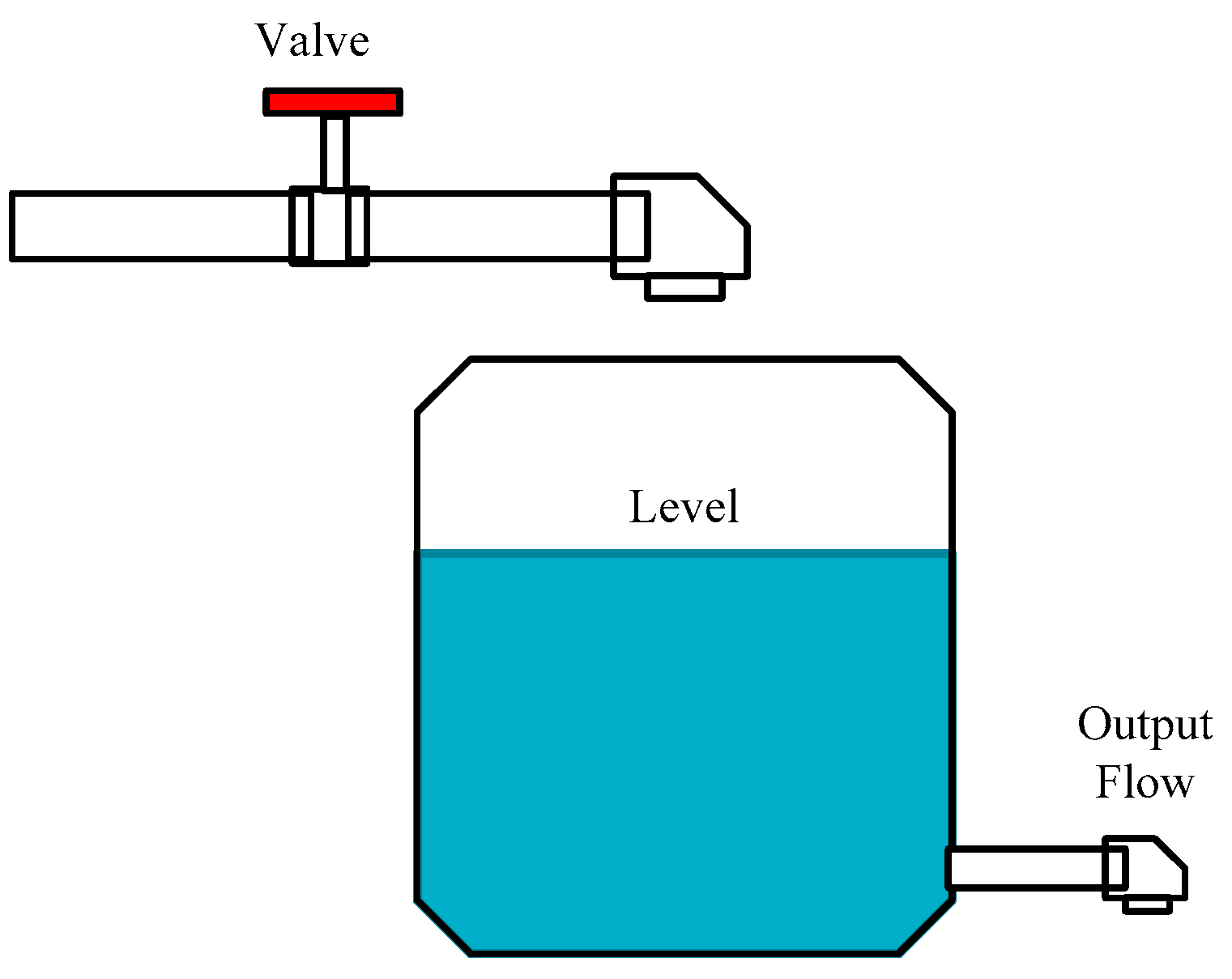
6. Water Level Control in a Tank
The water level control in a tank, illustrated in Figure 4, is a classical benchmark control problem and has been considered as a study case to improve the performance of FLC controllers and to compare FLC T1 and FLC T2, and other works with this plant can be found in [24,25].
The main formulation of this plant is expressed in Equation (17).
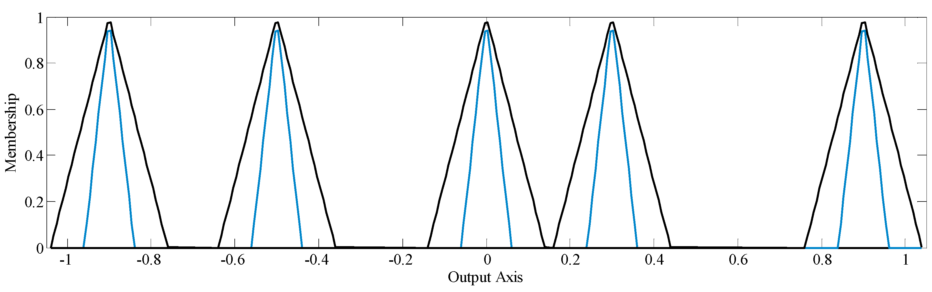
The output fuzzy set contains five MFs that are distributed without intersections as illustrated in Figure 5.
• Step 1
Define the partial knowledge of the system; and this can be expressed in Equations (18)–(22).
• Step 2
Table 3 defines the intervals of the partial knowledge and their functions. In this case, the number of intervals is double the number of MFs because these are composed functions.
• Step 3
In this case study, step 3 is not necessary because the MFs do not have intersections.
• Step 4
• Step 5
Equation (23) expresses and and and
is in an empty interval between 4 and 5, and is the 7th interval.
• Step 6
• Step 7
Using Table 3, Table 4, Table 5, Table 6 and Table 7 we applied Equations (13) and (14) to obtain Equations (24) and (25).
And after derivation we obtain Equations (26) and (27).
• Experiments.
In order to evaluate the proposed approximate CEKM type reductions, in this section, the proposed method is compared based on their computational cost, reliability with respect to the original method contrasted with other alternatives to reduce computational cost, and the control performance with respect to KM type reduction.
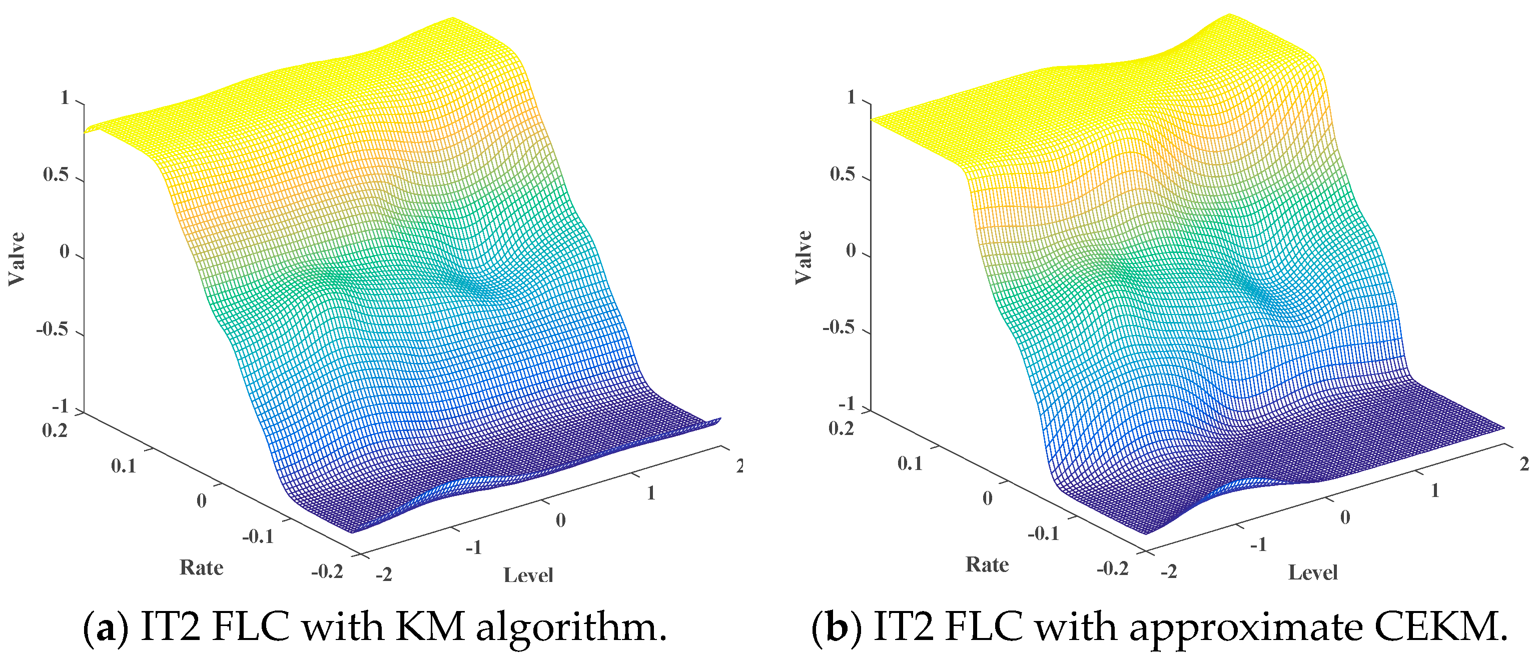
• Control surface comparison and execution time
The control surface represents the behavior of a controller, and is because of this reason that it is a very useful way to compare the proposed type-reduction approximation with respect to a classical type reduction, and Figure 6 illustrates both control surfaces.
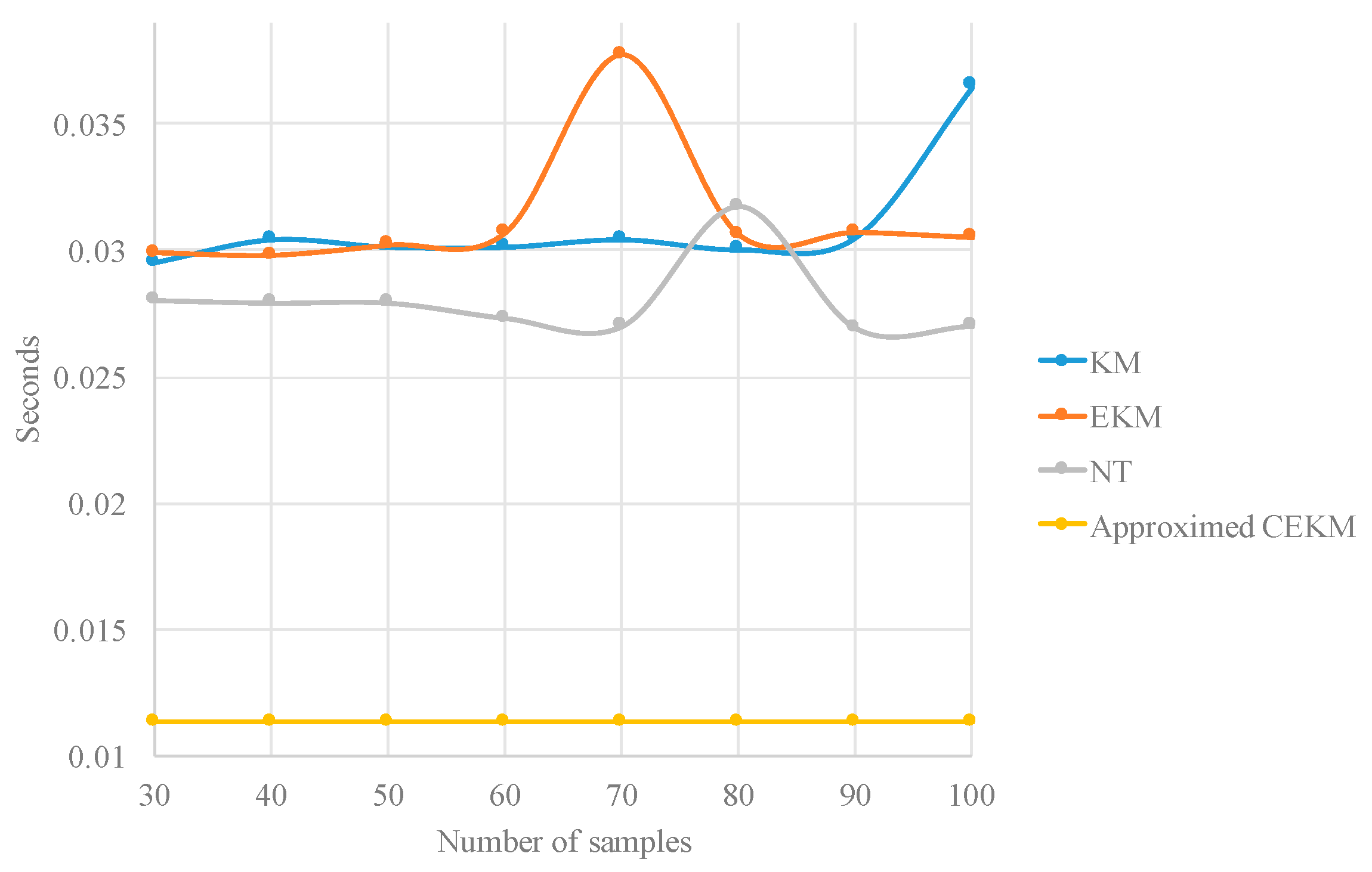
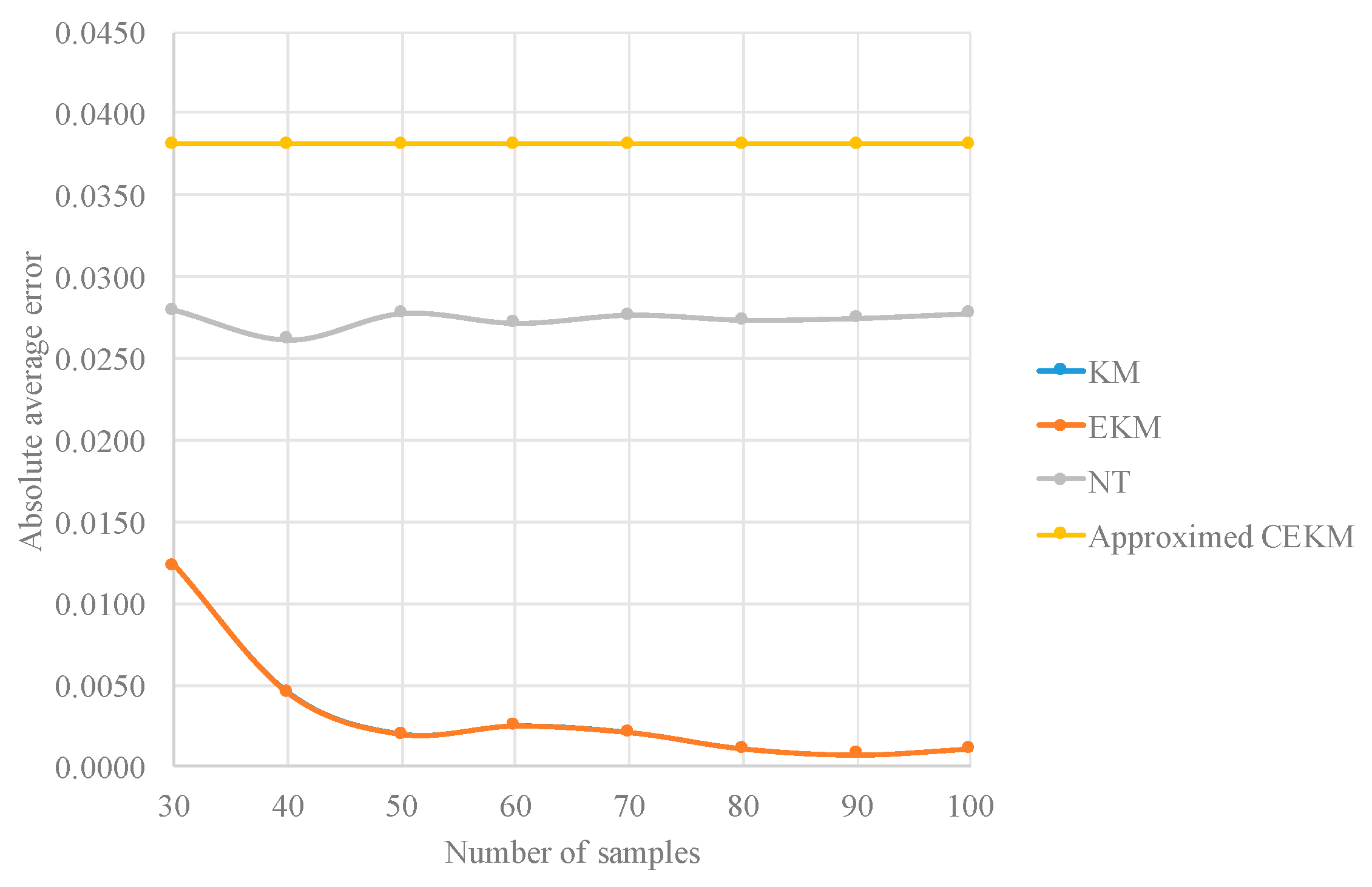
In Table 8, four type-reduction methods are compared by the absolute average errors with respect to a KM type reduction with ten thousand samples. The type-reduction methods that are compared are the KM, EKM, NT and the proposed approximate CEKM.
The experiments are realized by changing the number of samples of the type-reduction methods to observe their behavior in execution time and error, but remembering that the approximate CEKM type reduction is not iterative and does not requires sampling.
Figure 7 and Figure 8 illustrate the results reported 100 in Table 8, and as we can observe, the proposed approximate CEKM has the largest error (although note high), but is considerably faster.
• Performance comparison
On the other hand, we evaluate the performance of the KM algorithm with ten thousand samples.
Table 9, reports the results of the control performance and execution time in a simulation, and this performance is reported with the IAE, ITAE and RMSE control metrics.
In these experiments we can observe that the IT2 FLC with EKM TR obtains better performance results with respect to the same controller with approximated CEKM TR, however, the proposed alternative reduces the execution time of the IT2 FLC by 60%, which is good for real world problems.
7. Edge Detection
As another case study we are presenting image edge detection with IT2 fuzzy systems. Edge detection is a recent area of application with great results for IT2 fuzzy logic, and for example the works in [26,27,28].
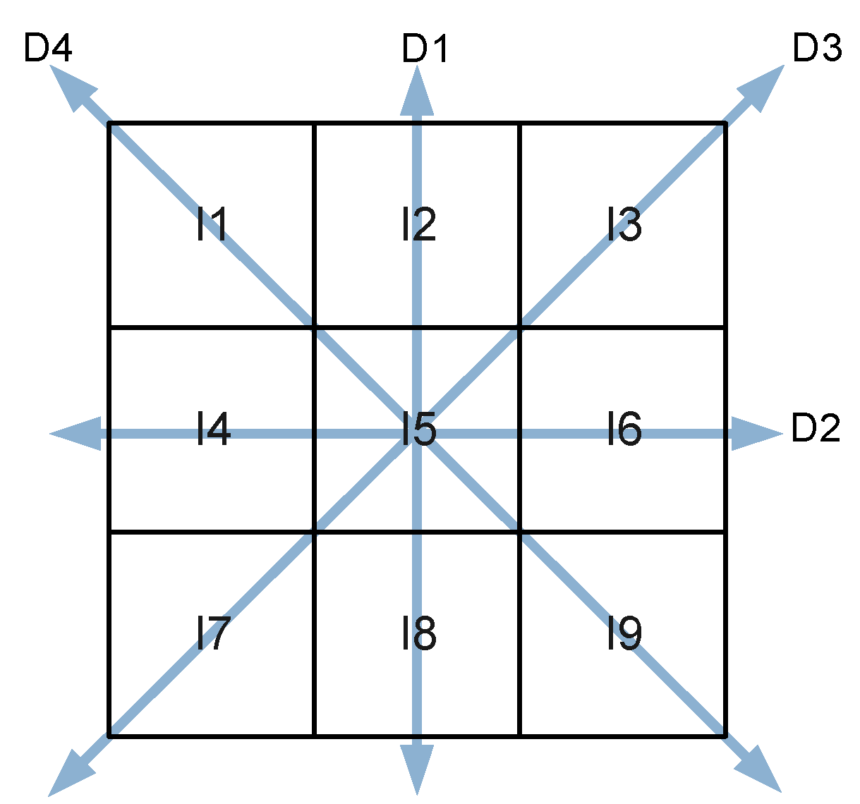
The IT2 FIS can be used to find if a pixel is or not an edge, and is necessary to consider the pixel’s neighborhood as shown in Figure 9.
This is because the pixel’s gradient is obtained as shown in Equation (28), this strategy, using the gradients is used for example in [6] and produces a good result.
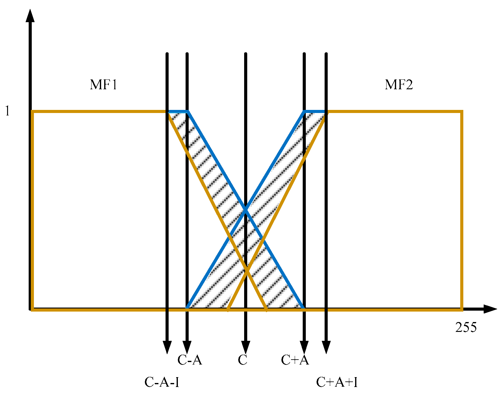
The gradients are approximated in this case as the differences in absolute values and these are the inputs to the IT2 FIS, the values are from 0 to 255, and the fuzzy sets can be found in Figure 10.
The MFs distribution for the fuzzy sets are the same for each input, and are parameterized as proposed in [6] allowing adaptation to different contexts.
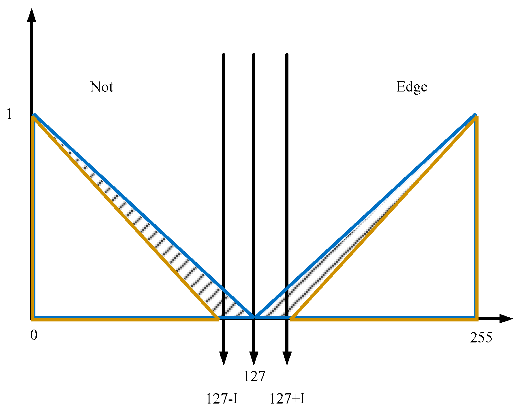
The proposed fuzzy sets are formed by two type-2 fuzzy membership functions as is shown in Figure 11.
As can be observed, the output fuzzy set is a composed function.
• Step 1
Equations (29) and (30) define the partial knowledge of the system.
• Step 2
Defines the output membership functions intervals, and these domains are reported in Table 10.
• Step 3
In this case, study, step 3 is not necessary because the MFs do not have intersections.
• Step 4
• Step 5
Equation (31) expresses and and
• Step 6
• Step 7
Using Table 10, Table 11, Table 12, Table 13 and Table 14 we propose the functions and , and these functions are expressed in Equations (32) and (33).
And Equations (34) and (35) express the derivatives of these functions.
Finally, we can define the approximate system outputs, and these equations are functions of the firing forces, and this eliminates the need to discretize and realize an iterative type reduction.
• Experiments
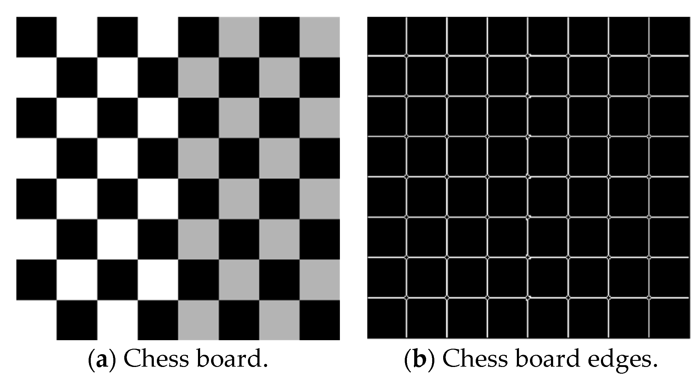
To evaluate the approximate CEKM Type Reduction, it is proposed to realize the edge detection based on the image illustrated in Figure 12, where the original image can be found and the corresponding obtained edges.
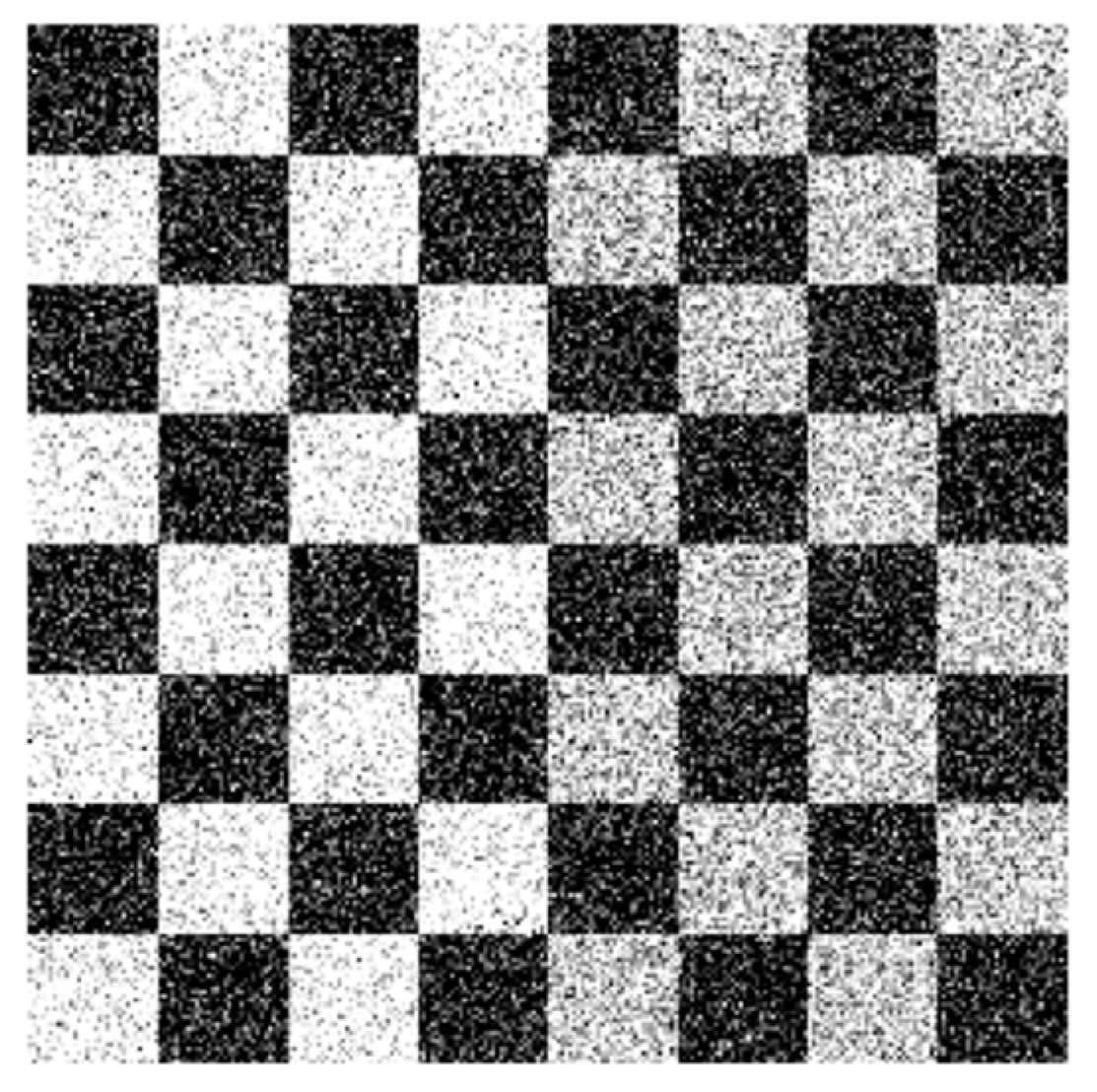
It is proposed to add Gaussian noise to the original image to test the performance of IT2 FLC in noisy environments, which in this case is a Gaussian noise with a variance of 0.1, and the illustration of these image plus noise can be appreciated in Figure 13.
Table 15 reports the results obtained by the edge detection of the image illustrated in Figure 13, the results are presented with a widely accepted performance metric known as Figure of Merit of Pratt (FOM) [29], and are compared with respect to the classical KM type reduction with ten thousand samples.
The FOM of both edge detectors is very similar, the percentage of equal pixels is 93.93%, however, the main results are in the execution time, with a reduction of 45% in the execution time and a competitive performance, and in this form the approximate CEKM Type Reduction shows an improvement with respect to EKM Type Reduction.
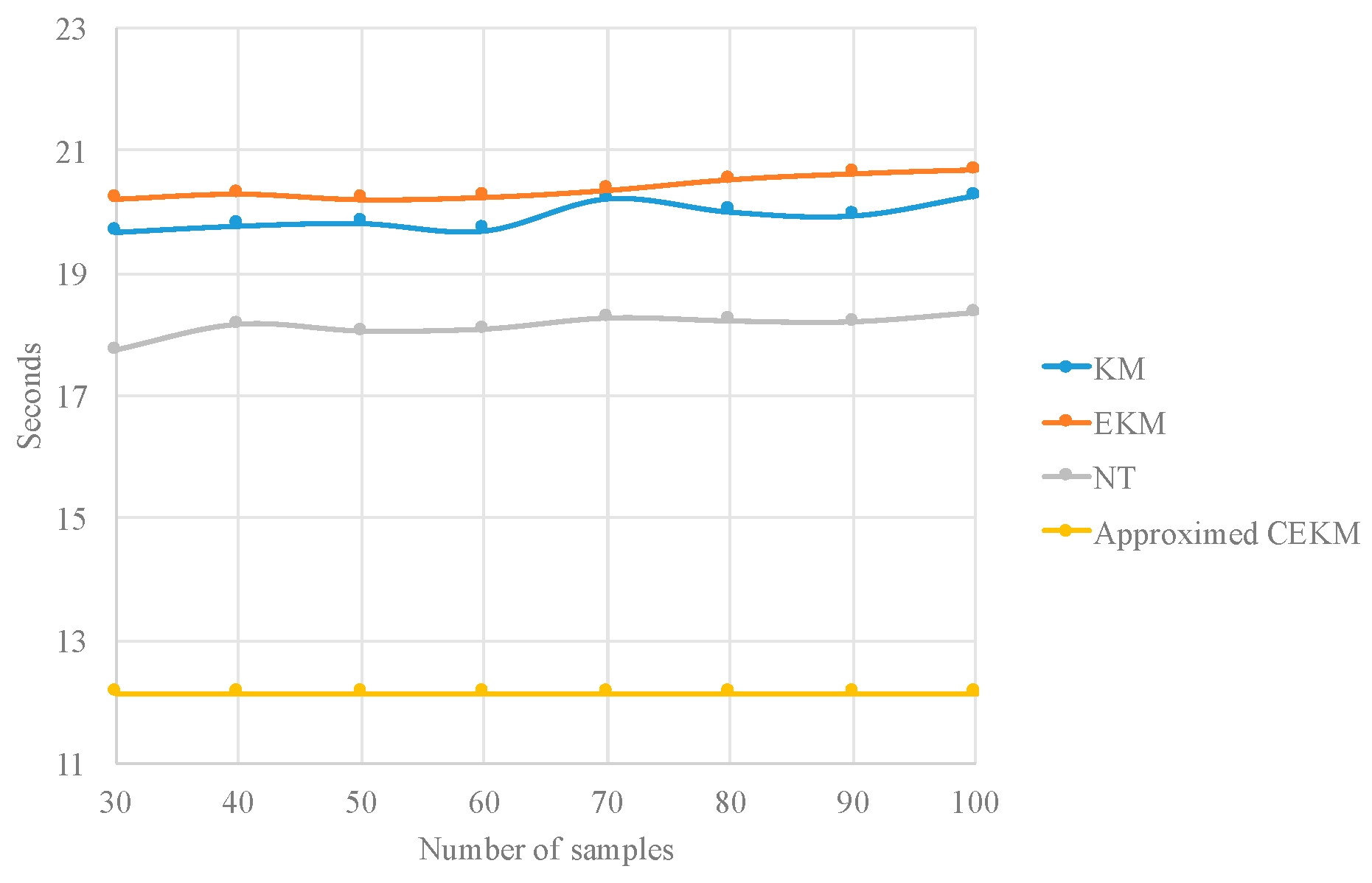
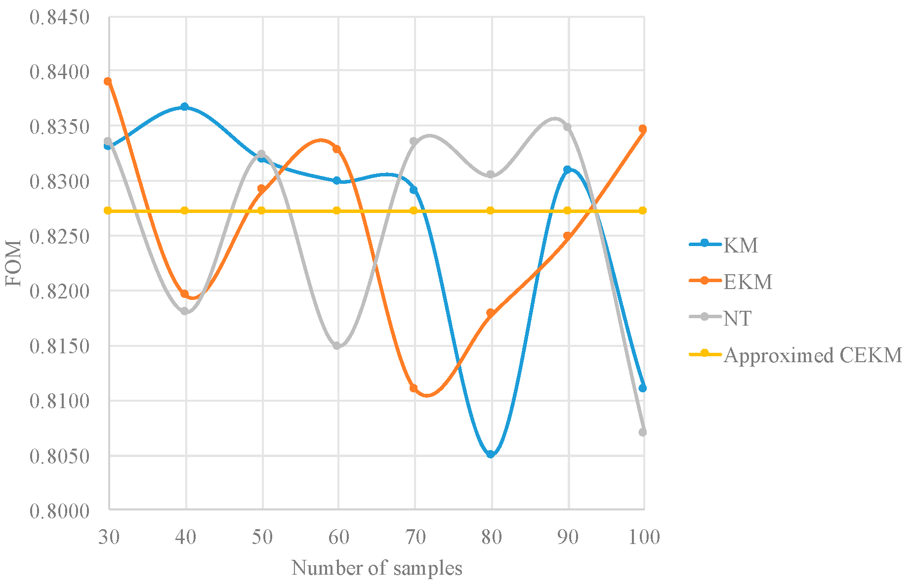
In order to compare the proposed approximate type reduction with respect to other improved type-reduction algorithms, these algorithms are also considered as alternatives to reduce the execution time of the process. The results are reported on Table 16. Figure 14 and Figure 15 illustrate, in a graphical way, the results reported on Table 16.
8. Conclusions
As a conclusion we have evaluated the proposed approximate CEKM type-reduction method with respect to the classical type-reduction algorithms and we can summarize the advantages and disadvantages in Table 17.
The proposed approximation is faster than other approximations, such as the NT Method. This is because it provides a continuous approximation of the output, which means that it not only eliminates the type-reduction process, but also reduces the defuzzification method to a polynomial, and on the other hand presents slightly higher error with respect to the theoretical model and other approximations. Based on the presented comparison we can state that the proposed algorithm is not recommended for:
- Applications where the error is a critical requirement.
- Applications that require adapting the IT2 FIS online.
We recommend the implementation of this approximate CEKM type-reduction algorithm in:
- Applications that require a high processing rate.
- Image processing applications that need calculation in real problems.
- Hardware implemented applications.
- Applications that execute the IT2 FIS as sub process.
Some examples of applications where the proposed approximation recommended is the use of fuzzy systems to make the parameters to be adaptive for a metaheuristic algorithm to optimize systems or mathematical functions [30,31,32,33,34]. This is because if, for example, the optimization takes one month, with the proposed approximation we can realize the same task in about two weeks, allowing to accelerate achieving the results of the research.
Acknowledgments
We would like to express our gratitude to CONACYT, Tijuana Institute of Technology for the facilities and resources granted for the development of this research.
Author Contributions
Oscar Castillo and Patricia Melin contributed to the discussion and analysis of the results; Emanuel Ontiveros-Robles proposed the approximation and methodology exposed in the present work, contributed to the simulations and wrote the paper.
Conflicts of Interest
The authors declare no conflict of interest.
References
- Castillo, O.; Melin, P. A review on the design and optimization of interval type-2 fuzzy controllers. Appl. Soft Comput. 2012, 12, 1267–1278. [Google Scholar] [CrossRef]
- Castillo, O.; Melin, P. A review on interval type-2 fuzzy logic applications in intelligent control. Inf. Sci. 2014, 279, 615–631. [Google Scholar] [CrossRef]
- Melin, P.; Castillo, O. A review on the applications of type-2 fuzzy logic in classification and pattern recognition. Expert Syst. Appl. 2013, 40, 5413–5423. [Google Scholar] [CrossRef]
- Sepúlveda, R.; Montiel, O.; Castillo, O.; Melin, P. Embedding a high speed interval type-2 fuzzy controller for a real plant into an FPGA. Appl. Soft Comput. 2012, 12, 988–998. [Google Scholar] [CrossRef]
- Maldonado, Y.; Castillo, O.; Melin, P. A multi-objective optimization of type-2 fuzzy control speed in FPGAs. Appl. Soft Comput. 2014, 24, 1164–1174. [Google Scholar] [CrossRef]
- Ontiveros-Robles, E.; Vázquez, J.G.; Castro, J.R.; Castillo, O. A FPGA-Based Hardware Architecture Approach for Real-Time Fuzzy Edge Detection. In Nature-Inspired Design of Hybrid Intelligent Systems; Melin, P., Castillo, O., Kacprzyk, J., Eds.; Springer: Berlin/Heidelberg, Germany, 2017; pp. 519–540. [Google Scholar]
- Melin, P. Image Processing and Pattern Recognition with Interval Type-2 Fuzzy Inference Systems. In Frontiers of Higher Order Fuzzy Sets; Sadeghian, A., Tahayori, H., Eds.; Springer: New York, NY, USA, 2015; pp. 217–228. [Google Scholar]
- Castillo, O.; Melin, P. Interval Type-2 Fuzzy Logic Applications. In Human-Centric Information Processing through Granular Modelling; Bargiela, A., Pedrycz, W., Eds.; Springer: Berlin/Heidelberg, Germany, 2009; pp. 203–231. [Google Scholar]
- Torshizi, A.D.; Zarandi, M.H.F.; Zakeri, H. On type-reduction of type-2 fuzzy sets: A review. Appl. Soft Comput. 2015, 27, 614–627. [Google Scholar] [CrossRef]
- Karnik, N.N.; Mendel, J.M. Type-2 fuzzy logic systems: type-reduction. In Proceedings of the 1998 IEEE International Conference on Systems, Man, and Cybernetics, San Diego, CA, USA, 11–14 October 1998; Volume 2, pp. 2046–2051. [Google Scholar]
- Wu, D.; Mendel, J.M. Enhanced Karnik-Mendel Algorithms for Interval Type-2 Fuzzy Sets and Systems. In Proceedings of the Annual Meeting of the North American Fuzzy Information Processing Society, San Diego, CA, USA, 24–27 June 2007; pp. 184–189. [Google Scholar]
- Khanesar, M.A.; Jalalian, A.; Kaynak, O.; Gao, H. Improving the Speed of Center of Set Type-Reduction in Interval Type-2 Fuzzy Systems by Eliminating the Need for Sorting. IEEE Trans. Fuzzy Syst. 2016. [Google Scholar] [CrossRef]
- Salaken, S.M.; Khosravi, A.; Nahavandi, S.; Wu, D. Linear approximation of Karnik-Mendel type reduction algorithm. In Proceedings of the IEEE International Conference on Fuzzy Systems, Istanbul, Turkey, 2–5 August 2015; pp. 1–6. [Google Scholar]
- Salaken, S.M.; Khosravi, A.; Nahavandi, S.; Wu, D. Switch point finding using polynomial regression for fuzzy type reduction algorithms. In Proceedings of the IEEE International Conference on Fuzzy Systems, Istanbul, Turkey, 2–5 August 2015; pp. 1–6. [Google Scholar]
- Nie, M.; Tan, W.W. Towards an efficient type-reduction method for interval type-2 fuzzy logic systems. In Proceedings of the IEEE International Conference on Fuzzy Systems (IEEE World Congress on Computational Intelligence), Hong Kong, China, 1–6 June 2008; pp. 1425–1432. [Google Scholar]
- Wu, D. An overview of alternative type-reduction approaches for reducing the computational cost of interval type-2 fuzzy logic controllers. In Proceedings of the IEEE International Conference on Fuzzy Systems, Brisbane, Australia, 10–15 June 2012; pp. 1–8. [Google Scholar]
- Mendel, J.M.; Liu, X. Simplified Interval Type-2 Fuzzy Logic Systems. IEEE Trans. Fuzzy Syst. 2013, 21, 1056–1069. [Google Scholar] [CrossRef]
- Liu, X.; Mendel, J.M. Connect Karnik-Mendel Algorithms to Root-Finding for Computing the Centroid of an Interval Type-2 Fuzzy Set. IEEE Trans. Fuzzy Syst. 2011, 19, 652–665. [Google Scholar]
- Zadeh, L.A. Fuzzy logic = computing with words. IEEE Trans. Fuzzy Syst. 1996, 4, 103–111. [Google Scholar] [CrossRef]
- Mendel, J.M.; John, R.I.B. Type-2 fuzzy sets made simple. IEEE Trans. Fuzzy Syst. 2002, 10, 117–127. [Google Scholar] [CrossRef]
- Mendel, J.M.; John, R.I.; Liu, F. Interval Type-2 Fuzzy Logic Systems Made Simple. IEEE Trans. Fuzzy Syst. 2006, 14, 808–821. [Google Scholar] [CrossRef]
- Karnik, N.N.; Mendel, J.M. Introduction to type-2 fuzzy logic systems. In Proceedings of the IEEE International Conference on Fuzzy Systems Proceedings. IEEE World Congress on Computational Intelligence (Cat. No.98CH36228), Anchorage, AK, USA, 4–9 May 1998; Volume 2, pp. 915–920. [Google Scholar]
- Liu, X.; Mendel, J.M.; Wu, D. Study on enhanced Karnik–Mendel algorithms: Initialization explanations and computation improvements. Inf. Sci. 2012, 184, 75–91. [Google Scholar] [CrossRef]
- Amador-Angulo, L.; Castillo, O. Optimization of the Type-1 and Type-2 fuzzy controller design for the water tank using the Bee Colony Optimization. In Proceedings of the IEEE Conference on Norbert Wiener in the 21st Century, Boston, MA, USA, 24–26 June 2014; pp. 1–8. [Google Scholar]
- Olivas, E.L.; Castillo, O.; Valdez, F.; Soria, J. Ant colony optimization for membership function design for a water tank fuzzy logic controller. In Proceedings of the IEEE Workshop on Hybrid Intelligent Models and Applications, Singapore, 16–19 April 2013; pp. 27–34. [Google Scholar]
- Mendoza, O.; Melin, P.; Licea, G. A New Method for Edge Detection in Image Processing Using Interval Type-2 Fuzzy Logic. In Proceedings of the IEEE International Conference on Granular Computing, Fremont, CA, USA, 2–4 November 2007; p. 151. [Google Scholar]
- Gonzalez, C.I.; Castro, J.R.; Mendoza, O.; Rodríguez-Díaz, A.; Melin, P.; Castillo, O. Edge detection method based on Interval type-2 fuzzy systems for color images. In Proceedings of the Annual Conference of the North American Fuzzy Information Processing Society (NAFIPS) held jointly with the 5th World Conference on Soft Computing (WConSC), Redmond, WA, USA, 17–19 August 2015; pp. 1–6. [Google Scholar]
- Melin, P.; Mendoza, O.; Castillo, O. An improved method for edge detection based on interval type-2 fuzzy logic. Expert Syst. Appl. 2010, 37, 8527–8535. [Google Scholar] [CrossRef]
- Perez-Ornelas, F.; Mendoza, O.; Melin, P.; Castro, J.R. Interval type-2 fuzzy logic for image edge detection quality evaluation. In Proceedings of the Annual Meeting of the North American Fuzzy Information Processing Society, Berkeley, CA, USA, 6–8 August 2012; pp. 1–6. [Google Scholar]
- Amador-Angulo, L.; Castillo, O. A new fuzzy bee colony optimization with dynamic adaptation of parameters using interval type-2 fuzzy logic for tuning fuzzy controllers. Soft Comput. 2016, 1–24. [Google Scholar] [CrossRef]
- Bernal, E.; Castillo, O.; Soria, J. Imperialist Competitive Algorithm with Dynamic Parameter Adaptation Applied to the Optimization of Mathematical Functions. In Nature-Inspired Design of Hybrid Intelligent Systems; Melin, P., Castillo, O., Kacprzyk, J., Eds.; Springer: Berlin/Heidelberg, Germany, 2017; pp. 329–341. [Google Scholar]
- Olivas, F.; Castillo, O. Particle Swarm Optimization with Dynamic Parameter Adaptation Using Fuzzy Logic for Benchmark Mathematical Functions. In Recent Advances on Hybrid Intelligent Systems; Castillo, O., Melin, P., Kacprzyk, J., Eds.; Springer: Berlin/Heidelberg, Germany, 2013; pp. 247–258. [Google Scholar]
- Ochoa, P.; Castillo, O.; Soria, J. Differential Evolution Using Fuzzy Logic and a Comparative Study with Other Metaheuristics. In Nature-Inspired Design of Hybrid Intelligent Systems; Melin, P., Castillo, O., Kacprzyk, J., Eds.; Springer: Berlin/Heidelberg, Germany, 2017; pp. 257–268. [Google Scholar]
- Peraza, C.; Valdez, F.; Castillo, O. An Adaptive Fuzzy Control Based on Harmony Search and Its Application to Optimization. In Nature-Inspired Design of Hybrid Intelligent Systems; Melin, P., Castillo, O., Kacprzyk, J., Eds.; Springer: Berlin/Heidelberg, Germany, 2017; pp. 269–283. [Google Scholar]
Figure 1.
Interval Type-2 Membership Function.

Figure 2.
Type-1 and Interval Type-2 Mamdani Fuzzy Inference Systems.

Figure 3.
Different types of composition operators.


Figure 4.
Water level tank control.

Figure 5.
Output membership fuctions.

Figure 6.
IT2 FLC control surfaces.

Figure 7.
Execution time comparison of the type-reduction algorithms.

Figure 8.
Average error comparison of the type-reduction algorithms.

Figure 9.
Neighborhood of a particular pixel.

Figure 10.
Fuzzy sets of the gradients.

Figure 11.
Output Fuzzy set.

Figure 12.
Test image and their edges detected.

Figure 13.
Test image plus noise.

Figure 14.
Execution time comparison for different type-reduction methods.

Figure 15.
FOM comparison for different type-reduction methods.


Table 1.
Karnik Mendel algorithm.
| Step | Left Point | Right Point |
|---|---|---|
| 1 | Sort by increasing order | Sort by increasing order |
| 2 | Initialize as: | Initialize as: |
| 3 | Compute: | Compute: |
| 4 | Find the switch point where | Find the switch point where |
| 5 | Set | Set |
| 6 | Compute: | Compute: |
| 7 | If then stop, set and , if not go to step 8. | If then stop, set and if not go to step 8. |
| 8 | Set and go to step 3. | Set and go to step 3. |
Table 2.
Proposed methodology.
| Step | Action |
|---|---|
| 1 | Define rules partial knowledge of the system. |
| 2 | Determinate the interval of each partial knowledge * Note: Considerate some interval can be composed. |
| 3 | Compute the intersection of the intervals obtained in step 2. The interceptions are determinate as the combination of the number of consequent membership functions. * Note: Several interceptions can contain empty domains. |
| 4 | Realize the integration of each interval, evaluating the defined integral the results are obtained in firing force’s function. |
| 5 | Found elements A and V. |
| 6 | Found and and and . |
| 7 | Compute Equations (8) and (9). |
Table 3.
Output MF intervals.
| Upper MFs | Lower MFs | ||
|---|---|---|---|
| Interval | Partial Knowledge | Interval | Partial Knowledge |
Table 4.
Upper MF integrals.
| I | Interval | Partial Knowledge | First Integral | Second Integral |
|---|---|---|---|---|
| 1 | ||||
| 2 | ||||
| 3 | ||||
| 4 | ||||
| 5 | ||||
| 6 | ||||
| 7 | ||||
| 8 | ||||
| 9 | ||||
| 10 |
Table 5.
Lower MF integrals.
| I | Interval | Partial knowledge | First Integral | Second Integral |
|---|---|---|---|---|
| 1 | ||||
| 2 | ||||
| 3 | ||||
| 4 | ||||
| 5 | ||||
| 6 | ||||
| 7 | ||||
| 8 | ||||
| 9 | ||||
| 10 |
Table 6.
and .
| I | Interval | ||
|---|---|---|---|
| 1 | |||
| 2 | |||
| 3 | |||
| 4 | |||
| 5 | |||
| 6 | |||
| 7 | |||
| 8 | |||
| 9 | |||
| 10 |
Table 7.
and .
| I | Interval | ||
|---|---|---|---|
| 1 | |||
| 2 | |||
| 3 | |||
| 4 | |||
| 5 | |||
| 6 | |||
| 7 | |||
| 8 | |||
| 9 | |||
| 10 |
Table 8.
Type reduction comparison.
| Samples | KM | EKM | NT | Approximate CEKM | ||||
|---|---|---|---|---|---|---|---|---|
| Time | E. Average | Time | E. Average | Time | E. Average | Time | E. Average | |
| 30 | 0.0295 | 0.0123 | 0.0299 | 0.0123 | 0.028 | 0.0279 | 0.0113 | 0.0381 |
| 40 | 0.0304 | 0.0045 | 0.0298 | 0.0045 | 0.0279 | 0.0261 | 0.0113 | 0.0381 |
| 50 | 0.0301 | 0.002 | 0.0302 | 0.002 | 0.0279 | 0.0277 | 0.0113 | 0.0381 |
| 60 | 0.0301 | 0.0025 | 0.0307 | 0.0025 | 0.0273 | 0.0271 | 0.0113 | 0.0381 |
| 70 | 0.0304 | 0.0021 | 0.0377 | 0.0021 | 0.027 | 0.0276 | 0.0113 | 0.0381 |
| 80 | 0.03 | 0.0011 | 0.0306 | 0.0011 | 0.0317 | 0.0273 | 0.0113 | 0.0381 |
| 90 | 0.0305 | 0.0007 | 0.0307 | 0.0007 | 0.0269 | 0.0274 | 0.0113 | 0.0381 |
| 100 | 0.0365 | 0.0011 | 0.0305 | 0.0011 | 0.027 | 0.0277 | 0.0113 | 0.0381 |
Table 9.
Performance comparison.
| KM Type Reduction | Approximate CEKM Type Reduction | ||
|---|---|---|---|
 |  | ||
| ISE | 1.9451 | ISE | 1.9691 |
| IAE | 2.9357 | IAE | 3.2730 |
| ITAE | 7.7548 | ITAE | 11.6868 |
| Time | 0.0322 s | Time | 0.0129 s |
Table 10.
Output intervals.
| Upper MFs | Lower MFs | |||
|---|---|---|---|---|
| Interval | Partial Knowledge | Interval | Partial Knowledge | |
| 1 | ||||
| 2 | ||||
Table 11.
and .
| Upper MFs | ||||
|---|---|---|---|---|
| Interval | Partial Knowledge | |||
| 1 | ||||
| 2 | ||||
Table 12.
and .
| Lower MFs | ||||
|---|---|---|---|---|
| Interval | Partial Knowledge | |||
| 1 | ||||
| 2 | ||||
Table 13.
and .
| Upper MFs | ||||
|---|---|---|---|---|
| Interval | Partial Knowledge | |||
| 1 | ||||
| 2 | ||||
Table 14.
and .
| Lower MFs | ||||
|---|---|---|---|---|
| Interval | Partial Knowledge | First Integral | Second Integral | |
| 1 | ||||
| 2 | ||||
Table 15.
Edge detection comparison with respect to classical KM type reduction.
| KM Type Reduction | Approximate CEKM Type Reduction | ||
|---|---|---|---|
 |  | ||
| FOM | 0.8269 | FOM | 0.8290 |
| Time | 22.9257 | Time | 12.6712 |
Table 16.
Edge detection comparison by variating the type-reduction method.
| Samples | KM | EKM | NT | Approximate CEKM | ||||
|---|---|---|---|---|---|---|---|---|
| Time | E. Average | Time | E. Average | Time | E. Average | Time | E. Average | |
| 30 | 19.6797 | 0.8331 | 20.2114 | 0.8389 | 17.7394 | 0.8335 | 12.1348 | 0.8272 |
| 40 | 19.7803 | 0.8366 | 20.2952 | 0.8195 | 18.1575 | 0.818 | 12.1348 | 0.8272 |
| 50 | 19.8204 | 0.8319 | 20.2071 | 0.8291 | 18.0473 | 0.8323 | 12.1348 | 0.8272 |
| 60 | 19.7011 | 0.8299 | 20.2435 | 0.8327 | 18.081 | 0.8149 | 12.1348 | 0.8272 |
| 70 | 20.2153 | 0.829 | 20.3531 | 0.8109 | 18.2579 | 0.8334 | 12.1348 | 0.8272 |
| 80 | 20.0018 | 0.805 | 20.5294 | 0.8178 | 18.2121 | 0.8304 | 12.1348 | 0.8272 |
| 90 | 19.9427 | 0.83 | 20.6222 | 0.8248 | 18.1986 | 0.8347 | 12.1348 | 0.8272 |
| 100 | 20.2376 | 0.811 | 20.6882 | 0.8346 | 18.3465 | 0.807 | 12.1348 | 0.8272 |
Table 17.
Advantages and Disadvantages of the Approximate CEKM method.
| Criteria | KM, CEKM, NT | Approximate CEKM |
|---|---|---|
| Error | Can obtain lowers errors | Have inherent errors |
| Iterations number | Depends the problem | Non iterative |
| Samples number | Error decreasing by increment the samples number | Do not requires sampling |
| Execution time | Increase by increment the samples number | Constant and significantly lower with respect to KM |
| Hardware implementation | Hardest to implement | Ideal for hardware implementation |
| Mathematical development | Does not require additional mathematical development | Requires a methodology to be able to implement it |
| Adaptation | Do not requires additional mathematical development | Requires to realize the methodology again to each variation |
© 2017 by the authors. Licensee MDPI, Basel, Switzerland. This article is an open access article distributed under the terms and conditions of the Creative Commons Attribution (CC BY) license (http://creativecommons.org/licenses/by/4.0/).
Share and Cite
MDPI and ACS Style
Ontiveros-Robles, E.; Melin, P.; Castillo, O. New Methodology to Approximate Type-Reduction Based on a Continuous Root-Finding Karnik Mendel Algorithm. Algorithms 2017, 10, 77. https://doi.org/10.3390/a10030077
AMA Style
Ontiveros-Robles E, Melin P, Castillo O. New Methodology to Approximate Type-Reduction Based on a Continuous Root-Finding Karnik Mendel Algorithm. Algorithms. 2017; 10(3):77. https://doi.org/10.3390/a10030077
Chicago/Turabian StyleOntiveros-Robles, Emanuel, Patricia Melin, and Oscar Castillo. 2017. "New Methodology to Approximate Type-Reduction Based on a Continuous Root-Finding Karnik Mendel Algorithm" Algorithms 10, no. 3: 77. https://doi.org/10.3390/a10030077
Note that from the first issue of 2016, this journal uses article numbers instead of page numbers. See further details here.