An Auto-Adjustable Semi-Supervised Self-Training Algorithm


1
Computer & Informatics Engineering Department, Technological Educational Institute of Western Greece, 263-34 GR Antirion, Greece
2
Department of Mathematics, University of Patras, 265-00 GR Patras, Greece
*
Author to whom correspondence should be addressed.
Algorithms 2018, 11(9), 139; https://doi.org/10.3390/a11090139
Submission received: 19 July 2018
/
Revised: 23 August 2018
/
Accepted: 10 September 2018
/
Published: 14 September 2018
(This article belongs to the Special Issue Humanistic Data Mining: Tools and Applications)
Abstract
:Semi-supervised learning algorithms have become a topic of significant research as an alternative to traditional classification methods which exhibit remarkable performance over labeled data but lack the ability to be applied on large amounts of unlabeled data. In this work, we propose a new semi-supervised learning algorithm that dynamically selects the most promising learner for a classification problem from a pool of classifiers based on a self-training philosophy. Our experimental results illustrate that the proposed algorithm outperforms its component semi-supervised learning algorithms in terms of accuracy, leading to more efficient, stable and robust predictive models.
1. Introduction
In machine learning and data mining, the construction of a classifier can be considered one of the most significant and challenging tasks [1]. Traditional classification algorithms belong to the class of supervised algorithms which use only labelled data to train the classifier. However, in many real-world classification problems, labelled instances are often difficult, expensive, or time consuming to obtain, since they require the efforts of empirical research. In contrast unlabeled data are fairly easy to obtain and require less effort of experienced human annotators.
Semi-supervised learning (SSL) algorithms constitute the appropriate and effective machine learning methodology for extracting knowledge from both labeled and unlabeled data so as to build efficient classifiers [2]. More analytically, they efficiently combine the explicit classification information of labeled data with the information hidden in the unlabeled data. The general assumption of this class of algorithms is that data points in a high density region are likely to belong to the same class and the decision boundary lies in low density regions [3]. Hence, these methods have the advantage of reducing the effort of supervision to a minimum, while still preserving competitive recognition performance. Nowadays, these algorithms have great interest both in theory and in practice and have become a topic of significant research as an alternative to traditional methods of machine learning, since they require less human effort and frequently present higher accuracy [4,5,6,7,8,9,10]. The main issue of semi-supervised learning is how to efficiently exploit the hidden information in the unlabeled data. In the literature, several approaches have been proposed with different philosophy related to the link between the distribution of labeled and unlabeled data [2,11,12,13,14].
Self-training constitutes perhaps the most popular and frequently used SSL algorithm due to its simplicity and classification accuracy [4,5,9]. This algorithm wraps around a base learner and uses its own predictions to assign labels to unlabeled data. More specifically, in the self-training process, a classifier is trained with a small number of labeled examples and iteratively enlarges its training set using newly labeled data with its own most confident predictions. However, this methodology can lead to erroneous predictions when noisy examples are classified as the most confident ones and in following incorporated into the labeled training set. Li and Zhou [15] tried to address this difficulty and presented the SETRED method which incorporates data editing in the self-training framework in order to actively learn from the self-labeled examples. Along this line, Tanha et al. [16] studied the classification behaviour of self-training and based on their numerical experiments, stated that the most important aspect of the self-training procedure is to correctly estimate the confidence of the predictions so as to be successful.
Therefore, the success of the self-training algorithm is depended on the newly labeled data [2] but most significantly, on the selection of the base learner. Nevertheless, the selection for base learner is still in progress since the decision of which particular learning algorithm to choose for a specific problem, is still a complicated and challenging problem. Given a pattern recognition problem, the traditional approach is to evaluate a set of different learners against a representative validation set and select the best one. It is generally recognized that the key to pattern recognition problems does not wholly lie in any particular solution since no single model exists for all problems [17].
In this work, we propose a new semi-supervised learning algorithm which is based on a self-training philosophy. The proposed algorithm initially uses several independent base learners and during the training process dynamically selects the most promising base learner relative to a strategy based on the number of the most confident predictions of unlabeled data. Our numerical experiments on several benchmark datasets confirm the efficacy of the proposed methodology. Additionally, we performed several statistical tests in order to illustrate the efficiency of our proposed algorithm.
The remainder of this paper is organized as follows: Section 2 defines the semi-supervised classification problem and the self-training approach. Section 3 presents a detailed description of the proposed algorithm and Section 4 presents the numerical experiments and discusses the obtained results. Finally, Section 5 discusses the conclusions and some further research topics for future work.
2. A Review of Semi-Supervised Classification Via Self-Labeled Approach
This section provides a definition for the semi-supervised classification problem and a short description of the most popular and frequently used semi-supervised self-labeled algorithms.
2.1. Semi-Supervised Classification
In the sequel, we present the definitions and the necessary notations for the semi-supervised classification problem. Let be an example, where belongs to a class y and a D-dimensional space in which is the i-th attribute of the p-th sample. Suppose L is a labeled set of instances with y known and U is an unlabeled set of instance with y unknown, where . Notice that the set consists the training set. Moreover, there is a test set T composed of unseen instances which has not been used in the training stage. The aim of semi-supervised classification is to obtain an accurate and robust learn hypothesis using the training set and in following evaluate its performance using the test set T.
In the literature, a variety of self-labeled methods has been proposed, each following a different methodology on exploiting the information hidden in the unlabeled data. Next, we present a brief description of the most popular and frequently used semi-supervised self-labeled methods.
2.2. Semi-Supervised Self-Labeled Methods
Self-training is a wrapper-based semi-supervised approach which constitutes an iterative procedure of self-labeling unlabeled data and is generally considered to be a simple and effective SSL algorithm. According to Ng and Cardie [18] “self-training is a single-view weakly supervised algorithm” which is based on its own predictions on unlabeled data to teach itself. In the self-training framework, an arbitrary classifier is initially trained with a small amount of labeled data which constitutes its training set, aiming to classify unlabeled points. Subsequently, it iteratively enlarges its labeled training set with its own most confident predictions and retrained. More specifically, at each iteration, the classifier’s training set is augmented gradually with classified unlabeled instances that have achieved a probability value over a defined threshold c; these instances are considered as sufficiently reliable to be added to the training set. Notice that the way in which the confidence predictions are measured depends on the type of used base learner (see [19]).
Clearly, this model does not make any specific assumptions for the input data, but rather accepts that its own predictions tend to be correct. Therefore, since the success of the self-training algorithm is heavily depended on the newly-labeled data based on its own predictions, its weakness is that erroneous initial predictions will probably lead the classifier to generate incorrectly labeled data [2].
Li and Zhou [15] tried to address this difficulty and as a result, they presented the SETRED method which incorporates data editing in the self-training framework in order to actively learn from the self-labeled examples. Their principal improvement in relation to the classical self-training scheme, is the establishment of a restriction related to the acceptance or the rejection of the unlabeled examples which are evaluated as trustworthy by the algorithm. More analytically, a neighboring graph in D-dimensional feature space is being built and all the candidate unlabeled examples for being appended to the initial training set are being filtered through a hypothesis test. Thus, any examples having successfully passed that test are finally added to the training set before the end of each iteration.
Co-training is a semi-supervised algorithm which can be regarded as a different variant of the self-training technique [12]. It is based on the strong assumption that the feature space can be divided into two conditionally independent views, with each view being sufficient to train an efficient classifier. In this framework, two learning algorithms are separately trained for each view using the initial labeled dataset and the most confident predictions of each algorithm on unlabeled data are used to augment the training set of the other through an iterative learning process. Following the same concept, Nigam and Ghani [14] performed an experimental analysis where they concluded that the Co-training outperforms other SSL algorithms when there is a natural existence of two distinct and independent views. Nevertheless, the assumption about the existence of sufficient and redundant views is a luxury hardly met in most real-case scenarios.
Zhou and Goldman [20] have also adopted the idea of ensemble learning and majority voting in the semi-supervised framework. Along this line, Li and Zhou [21] proposed another algorithm, in which several Random Trees are trained on bootstrap data from the dataset, named Co-Forest. The main idea of this algorithm is the assignment of a few unlabeled examples to each Random Tree during the training process. Eventually, the final decision is composed by a simple majority voting. Notice that the use of Random Tree classifier for random samples of the collected labeled data is the main reason why the behavior of Co-Forest is efficient and robust although the number of the available labeled examples is reduced.
A rather representative approach which is based on the ensemble philosophy is the Tri-training algorithm. This algorithm constitutes an improved single-view extension of the Co-training algorithm exploiting unlabeled data without relying on the existence of two views of instances [22]. Tri-training algorithm can be considered as a bagging ensemble of three classifiers which are trained on data subsets generated through bootstrap sampling from the original labeled training set [23]. Subsequently, in each Tri-training round, if two classifiers agree on the labeling of an unlabeled instance while the third one disagrees, then these two classifiers will label this instance for the third classifier. It is worth noticing that the “majority teach minority strategy” serves as an implicit confidence measurement which avoids the use of complicated time-consuming approaches for explicitly measuring the predictive confidence, and hence the training process is efficient [4].
3. Auto-Adjustable Self-Training Semi-Supervised Algorithm
In this section, we present the proposed SSL algorithm which is based on the self-training framework. We recall that two main difficulties in self-training is the decision of which base learner to choose for a specific problem and how to find a set of high confidence predictions of unlabeled data. Therefore, in order to address these difficulties, we consider starting with an initial pool of classifiers and during the training process, to dynamically select the most promising classifier, relative to the most confident predictions. A high-level description of the proposed semi-supervised algorithm, entitled Auto-Adjustable Self-Training (AAST), is presented in Algorithm 1 which consists of two phases: in the 1st phase, the most promising classifier is selected from a pool of classifiers based on the number of confident predictions of unlabeled data, whereas in the 2nd phase, the most promising classifier is trained within the self-training framework.
Suppose that constitutes a set of N classifiers which can be used as base learners in the self-training framework. Initially, all base learners are trained using the same small amount of labeled data L and then applied on the same unlabeled data U. Subsequently, the labeled set of each classifier is iteratively augmented gradually using its own most confident predictions. More specifically, each classified unlabeled instance that has achieved a probability value over a defined threshold c, is considered sufficiently reliable in order to be added to the classifier’s labeled set for the following training phases. It is worth mentioning that the way the confidence predictions are measured, depends on the type of the used base learner (see [19,27,28] and the references there in). Finally, each classifier is re-trained using its own new enlarged training set.
| Algorithm 1: Auto-Adjustable Self-Training (AAST). |
|
The proposed algorithm in order to select a base learner from set C is grounded on the following simple idea: the most promising base learner is probably the base learner with the most confident predictions. In other words, the base learner that is able to confidently label as many unlabeled instances as possible in order to explore them is the most promising classifier.
Every k iterations (which we call a cycle), AAST evaluates the base learner in set C and selects the classifier with the minimum number of most confident predictions as well as the classifier with the maximum number of most confident predictions. Subsequently, the classifier is removed from the set C and the classifier will provide its labeled set and its unlabeled set for all the rest classifiers for the next cycle. More to the point, in every cycle (i.e., every k iterations) the algorithm removes the least promising classifier from the set C, in order to reduce the computational cost and restarts the self-training process using the labeled and unlabeled sets of the most promising classifier , relative to the number of most confident predictions of each classifier.
Notice that, it is immediately implied from the above discussion that after cycles (i.e., iterations), where is the initial number of used base learners, only one classifier, denoted as , remains in set C. This classifier constitutes the most promising classifier, relative to the proposed selection strategy. Subsequently, the only remaining classifier continues its training within the semi-supervised framework.
An obvious advantage of the proposed technique is that it exploits the diversity of the errors of the learned models by using different learning algorithms and the classifier with the most confident predictions is dynamically selected as the most promising one. Nevertheless, the efficacy and computational cost of the proposed algorithm depends on the value of parameter k. As the value of parameter k increases, the base learners exploit the hidden information in the unlabeled data for more iterations before being evaluated; however, the computational cost and time significantly increases.
4. Experimental Results
The experiments were based on 40 datasets from UCI Machine Learning Repository [29] and KEEL repository [30]. Table 1 presents a brief description of the datasets’ structure i.e., the number of instances (#Instances), number of attributes (#Features) and number of output classes (#Classes). The considered datasets contain between 101 and instances, while the number of attributes ranges from 2 to 60 and the number of classes varies between 2 and 11.
Our experimental results were obtained by conducting a three phase procedure: In the first phase, the performance of the proposed algorithm AAST using various values of parameter k in order to study its sensitivity is evaluated; in the second phase, the performance of AAST with that of the most popular and commonly used self-labeled algorithms is compared, while in the third stage, a statistical comparison between all compared semi-supervised self-labeled algorithms is performed. The detailed numerical results can be found in the web site: www.math.upatras.gr/~livieris/Results/AAST.zip.
The implementation code was written in Java, using the WEKA Machine Learning Toolkit [28] and the classification accuracy was evaluated using the stratified 10-fold cross-validation i.e., the data was separated into folds so that each fold had the same distribution of classes as the entire dataset. For each generated fold, a given algorithm is trained with the examples contained in the rest of the other folds (training partition) and then tested with the current fold. Moreover, the training partition was divided into labeled and unlabeled subsets.
Similar to [13,31] in the division process, we do not maintain the class proportion in the labeled and unlabeled sets since the main aim of semi-supervised classification is to exploit unlabeled data for better classification results. Hence, we use a random selection of examples that will be marked as labeled instances and the class label of the remaining instances will be removed. Furthermore, we ensure that every class has at least one representative instance. To study the influence of the amount of labeled data, three different ratios R were used: , and . In summary, this experimental study involves a total of 120 datasets (40 datasets × 3 labeled ratios).
Furthermore, the proposed algorithm uses three well-known supervised classifiers as base learners namely C4.5, JRip and kNN. These base learners constitute some of the most effective and widely used data mining algorithms for classification [24,32]. A brief description of these classifiers is given below:
- C4.5 [33] constitutes one of the most effective and efficient classification algorithms for building decision trees. This algorithm induces classification rules in the form of decision trees for a given training set. More analytically, it categorizes instances to a predefined set of classes according to their attribute values from the root of a tree down to a leaf. The accuracy of a leaf corresponds to the percentage of correctly classified instances of the training set.
- JRip [34] is generally considered to be a very effective and fast rule-based algorithm, especially on large samples with noisy data. The algorithm examines each class in increasing size and an initial set of rules for a class is generated using incremental reduced errors. Then, it proceeds by treating all the examples of a particular judgement in the training data as a class and determines a set of rules that covers all the members of that class. Subsequently, it proceeds to the next class and iteratively applies the same procedure until all classes have been covered. What is more, JRip produces error rates competitive with C4.5 with less computational effort.
- kNN [35] constitutes a representative instance-structured learning algorithm based on dissimilarities among a set of instances. It belongs to the lazy learning family of methods [35] which do not build a model during the learning process. According to kNN algorithm, characteristics extracted from classification process by viewing the entire distance among new individuals, should be classified and then the nearest k category is used. As a result of this process, test data belongs to the nearest k neighbor category which has more members in certain class. The main advantages of the kNN classification algorithm is its easiness and simplicity of implementation and the fact that it provides good generalization results during classification assigned to multiple categories.
The configuration parameters of the proposed algorithm AAST and base learners used in the experiments are presented in Table 2. Moreover, similar to Blum and Mitchell [12], we established a limit to the number of iterations (MaxIter = 40), in algorithm AAST.
All classification algorithms were evaluated using the performance profiles based on accuracy proposed by Dolan and Morè [36]. This metric provides a wealth of information such as solver efficiency, robustness and probability of success in compact form. More specifically, authors presented a new tool for analyzing the efficiency of algorithms by introducing the notion of a performance profile as a means to evaluate and compare the performance of the set of solvers S on a test set P.
Assuming that there exist solvers and problems for each solver s and problem p, they defined as the percentage of misclassified instances by solver s for problem p. Requiring a baseline for comparisons, they compared the performance on problem p by solver s with the best performance by any solver on this problem; that is, using the performance ratio.
The performance of solver s on any given problem might be of interest, but we would like to obtain an overall assessment of the performance of the solver. Next they defined.
Function was the (cumulative) distribution function for the performance ratio. The performance profile for a solver was a non-decreasing, piecewise constant function, continuous from the right at each breakpoint [36]. In other words, the performance profile plots the fraction P of problems for which any given method is within a factor of the best solver. According to the above rules and discussion, we conclude that one solver whose performance profile plot is on top right will win over the rest of the solvers.
Ultimately, the use of performance profiles eliminates the influence of a small number of problems on the benchmarking process and the sensitivity of results associated with the ranking of solvers [36,37,38]. It is worth mentioning that the vertical side of a performance profile gives the percentage of the problems that were successfully solved by each method (robustness).
4.1. Sensitivity of AAST to the Value of Parameter k
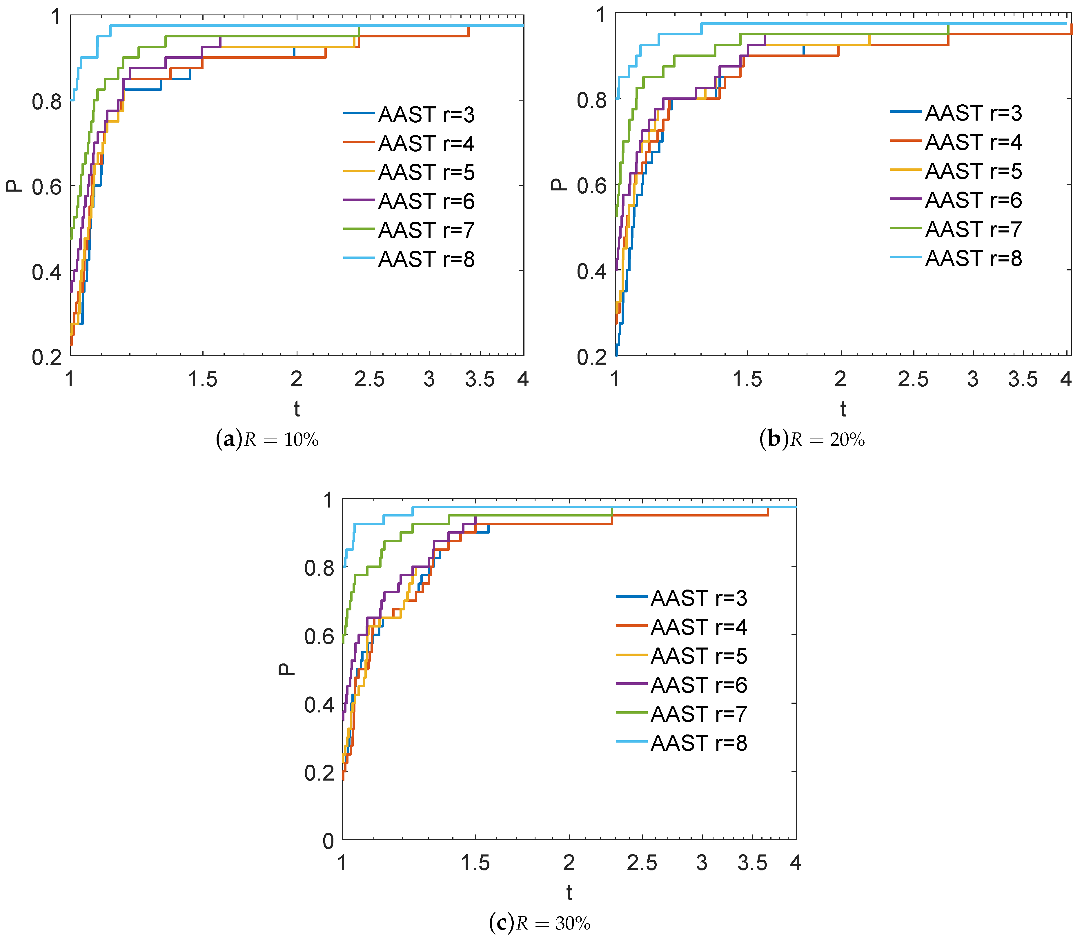
In the sequel, we focus our interest on the experimental analysis for the best value of parameter k; hence, we have tested values of k ranging from 3 to 8 in steps of 1. Figure 1 presents the performance profiles for various values of parameter k, relative to the used ratio of labeled data. Clearly, AAST exhibits better classification performance as the value of parameter k increases, revealing its sensitivity. More specifically, using as labeled ratio, AAST with and 8 classifies , , , , and of the test problems with the highest accuracy, respectively. Furthermore, AAST with and 8 classifies , , , , and of the test problems with the highest accuracy, respectively for labeled ratio as well as , , , , and , respectively for labeled ratio.
4.2. Performance Evaluation of AAST
Subsequently, we evaluate the performance of the proposed algorithm AAST against Self-training using C4.5, JRip and kNN as base learners. In the rest of this section, the value of parameter k in Algorithm AAST is set to 8 which exhibited the highest classification accuracy.
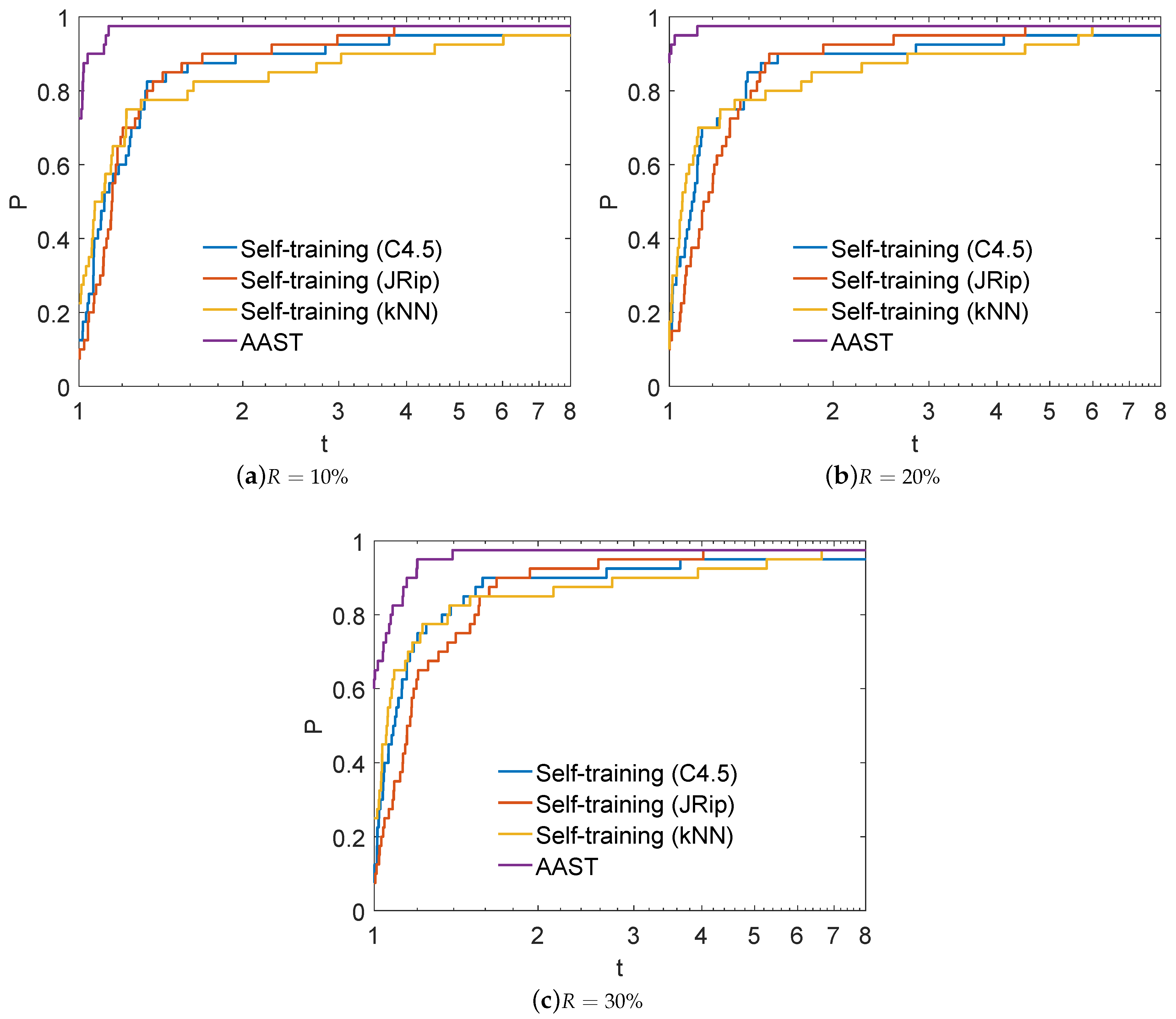
Figure 2 presents the performance profiles for Self-training and AAST. Obviously, AAST illustrates the highest probability of being the optimal classifier since it corresponds to the top curve, regarding all used labeled ratio. More analytically, AAST reports the best performance, classifying , and of the test problems with the highest accuracy using , and as labeled ratio, respectively, followed by Self-training (kNN) reporting , and , in the same situations.
Finally, in order to demonstrate the classification performance of the proposed algorithm, we compare it with other state-of-the-art self-labeled algorithms such as Co-training [12] and Tri-training [22] using C4.5, JRip and kNN as base learners, Co-Forest [21] and SETRED [15]. Notice that all algorithms were used with the parameters presented in [30].
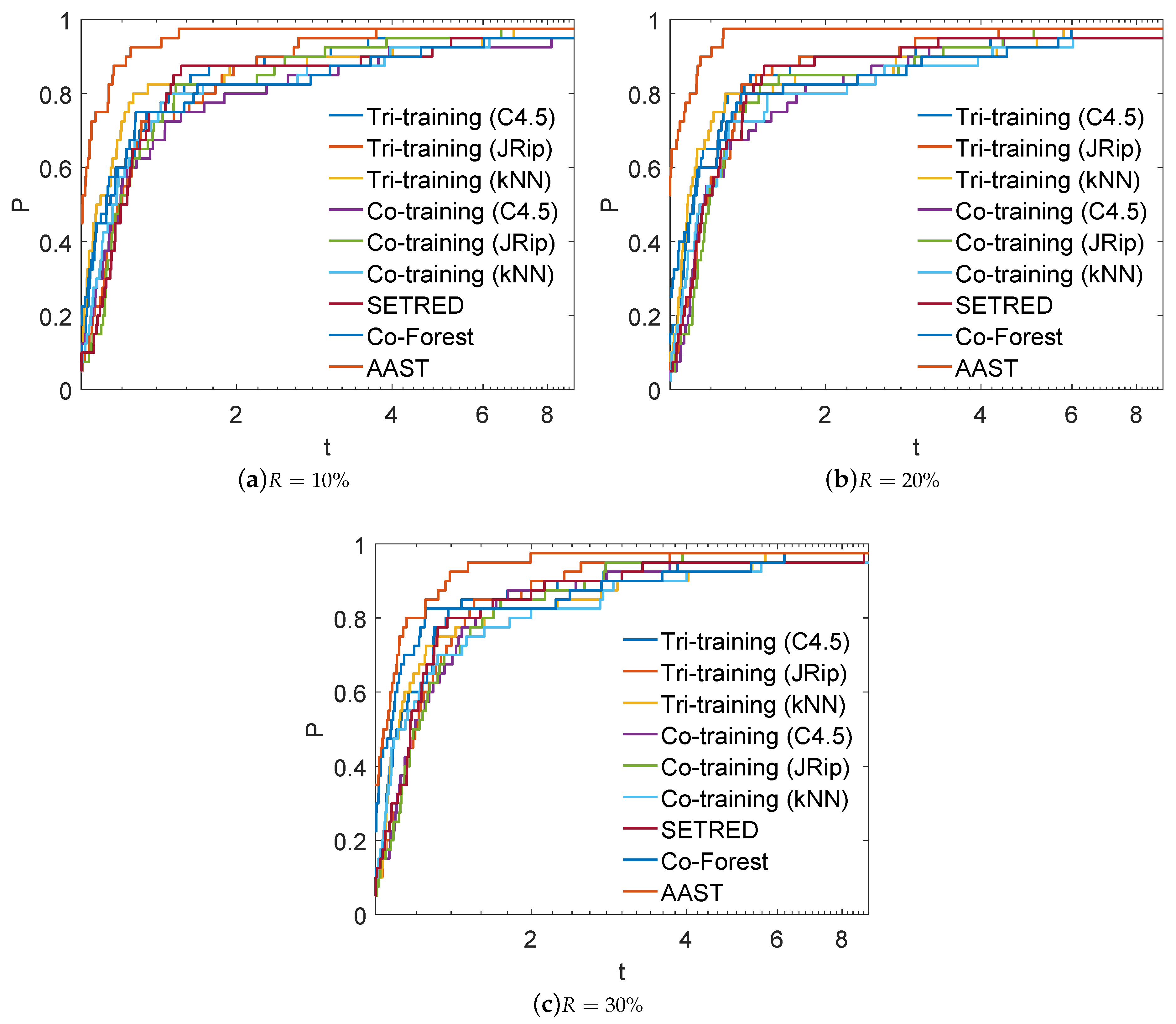
Figure 3 presents the performance profiles of some state-of-the-art self-labeled algorithms and AAST, regarding the used labeled ratio. Despite the ratio of instances, AAST algorithm managed to achieve the best overall performance, outperforming all self-labeled algorithms. More specifically, AAST classifies , and of the test problems with the highest accuracy, using , and as labeled ratio, respectively. Conclusively, it is worth mentioning that the reported performance profiles illustrate that AAST exhibits better performance on average, outperforming classical SSL methods, but this is not in general the case for a single dataset.
4.3. Statistical and Post-Hoc Analysis
The statistical comparison of multiple algorithms over multiple datasets is fundamental in machine learning and usually it is carried out by means of a non-parametric statistical test. Therefore, we use Friedman Aligned-Ranks (FAR) test [39] in order to conduct a complete performance comparison between all algorithms for all the different labeled ratios. Its application will allow us to highlight the existence of significant differences between our proposed algorithm and the classical SSL algorithms and in following to evaluate the rejection of the hypothesis that all the classifiers perform equally well for a given level [25,40].
Let be the rank of the j-th of k learning algorithms on the i-th of M problems. Under the null-hypothesis which states that all the algorithms are equivalent, the Friedman aligned ranks test statistic is defined by:
where is equal to the rank total of the i-th dataset and is the rank total of the j-th algorithm. The test statistic is compared with the distribution with degrees of freedom. Please note that since the test is non-parametric, it does not require the commensurability of the measures across different datasets. In addition, this test does not assume the normality of the sample means, and thus, it is robust to outliers.
In statistical hypothesis testing, the p-value is the probability of obtaining a result at least as extreme as the one that was actually observed, while assuming that the null hypothesis is true. In other words, the p-value provides information about whether a statistical hypothesis test is significant or not, thus indicating “how significant” the result is while it does this without committing to a particular level of significance. When a p-value is considered in a multiple comparison, it reflects the probability error of a certain comparison; however, it does not take into account the remaining comparisons belonging to the family. One way to address this problem is to report adjusted p-values which take into account that multiple tests are conducted and can be compared directly with any significance level [40].
To this end, the Finner Post-Hoc test [39] with a significance level was applied so as to detect the specific differences between the algorithms. In addition, the Finner test is easy to comprehend, as it usually offers better results than other Post-Hoc tests, especially when the number of compared algorithms is low [40]. The Finner procedure adjusts the value of in a step-down manner. Let be the ordered p-values with and be the corresponding hypothesis. The Finner procedure rejects – if i is the smallest integer such that , while the adjusted Finner p-value is defined by:
where is the p-value obtained for the j-th hypothesis and . It is worth mentioning that the test rejects the hypothesis of equality when the adjusted Finner p-value is less than .
Table 3, Table 4 and Table 5 present the information of the statistical analysis performed by non-parametric multiple comparison procedures over , and of labeled data, respectively. The best (lowest) ranking obtained in each FAR test determines the control algorithm for the Post-Hoc test. Moreover, the adjusted p-value with Finner’s test (Finner APV) is presented based on the control algorithm, at level of significance. Clearly, the proposed algorithm exhibits the best overall performance, outperforming the rest self-labeled algorithms, since it reports the highest probability-based ranking and presents statistically better results, relative to all labeled ratio.
5. Conclusions and Future Research
In this work, we presented a new SSL algorithm which is based on a self-training philosophy. More specifically, our proposed algorithm automatically selects the best base learner, relative to the number of the most confident predictions of unlabeled data.
The efficiency of the proposed semi-supervised algorithm was evaluated on several benchmark datasets in terms of classification accuracy utilizing the most frequently used base learners: C4.5, kNN and JRip and different ratios of labeled data. Our numerical results as well as the presented statistical analysis demonstrate that the AAST algorithm outperforms its component SSL algorithms, confirming the effectiveness and robustness of the proposed method. Therefore, the presented methodology seems to lead to more efficient, stable and robust predictive models.
In our future work, we intend to pursue extensive empirical experiments in order to compare the proposed self-labeled method AAST with various methods, belonging to other SSL classes such as generative mixture models [14,41], transductive SVMs [42,43,44], graph-based methods [45,46,47,48,49], extreme learning methods [50,51,52], expectation maximization with generative mixture models [14,53]. Furthermore, since our experimental results are quite encouraging, our next step is the use of other supervised classifiers as base learners, such as neural networks [54] and support vector machines [55] or ensemble-based learners [26] aiming to enhance our proposed framework with more sophisticated and theoretically motivated selection criteria for the most promising classifier in order to study the behavior of AAST at each cycle. Finally, an interesting aspect is the evaluation of the proposed algorithm in specific scientific fields applying real world datasets, such as educational, health care, etc. and explore its performance on imbalanced datasets [56,57] using more sophisticated performance metrics such as Sensitivity, Specificity, F-measure, AUC, ROC curve [58,59].
Author Contributions
I.E.L., A.K., V.T. and P.P. conceived of the idea, designed and performed the experiments, analyzed the results, drafted the initial manuscript and revised the final manuscript.
Funding
This research received no external funding.
Conflicts of Interest
The authors declare no conflict of interest.
References
- Alpaydin, E. Introduction to Machine Learning, 2nd ed.; The MIT Press: Cambridge, MA, USA, 2010. [Google Scholar]
- Zhu, X.; Goldberg, A. Introduction to semi-supervised learning. Synth. Lect. Artif. Intell. Mach. Learn. 2009, 3, 1–130. [Google Scholar] [CrossRef]
- Zhu, X. Semi-supervised learning. In Encyclopedia of Machine Learning; Springer: Berlin, Germany, 2011; pp. 892–897. [Google Scholar]
- Livieris, I.E.; Drakopoulou, K.; Tampakas, V.; Mikropoulos, T.; Pintelas, P. Predicting secondary school students’ performance utilizing a semi-supervised learning approach. J. Educ. Comput. Res. 2018. [Google Scholar] [CrossRef]
- Sigdel, M.; Dinç, I.; Dinç, S.; Sigdel, M.; Pusey, M.; Aygün, R. Evaluation of semi-supervised learning for classification of protein crystallization imagery. Proc. IEEE Southeastcon 2014, 1–6. [Google Scholar] [CrossRef]
- Keyvanpour, M.; Imani, M. Semi-supervised text categorization: Exploiting unlabeled data using ensemble learning algorithms. Intell. Data Anal. 2013, 17, 367–385. [Google Scholar]
- Hassanzadeh, H.; Keyvanpour, M. A two-phase hybrid of semi-supervised and active learning approach for sequence labeling. Intell. Data Anal. 2013, 17, 251–270. [Google Scholar]
- Borchani, H.; Larrañaga, P.; Bielza, C. Classifying evolving data streams with partially labeled data. Intell. Data Anal. 2011, 15, 655–670. [Google Scholar]
- Chen, M.; Tan, X.; Zhang, L. An iterative self-training support vector machine algorithm in brain-computer interfaces. Intell. Data Anal. 2016, 20, 67–82. [Google Scholar] [CrossRef]
- Laleh, N.; Azgomi, M.A. A hybrid fraud scoring and spike detection technique in streaming data. Intell. Data Anal. 2010, 14, 773–800. [Google Scholar]
- Blum, A.; Chawla, S. Learning from Labeled and Unlabeled Data Using Graph Mincuts. In Proceedings of the 18th International Conference on Machine Learning, Williamstown, MA, USA, 28 June–1 July 2001; Morgan Kaufmann Publishers Inc.: Burlington, MA, USA; pp. 19–26. [Google Scholar]
- Blum, A.; Mitchell, T. Combining labeled and unlabeled data with co-training. In Proceedings of the 11th Annual Conference on Computational Learning Theory, Madison, WI, USA, 24–26 July 1998; ACM: New York, NY, USA, 1998; pp. 92–100. [Google Scholar] [Green Version]
- Triguero, I.; García, S.; Herrera, F. Self-labeled techniques for semi-supervised learning: taxonomy, software and empirical study. Knowl. Inf. Syst. 2015, 42, 245–284. [Google Scholar] [CrossRef]
- Nigam, K.; Ghani, R. Analyzing the effectiveness and applicability of co-training. In Proceedings of the 9th International Conference on Information and Knowledge Management, McLean, VA, USA, 6–11 November 2000; ACM: New York, NY, USA, 2000; pp. 86–93. [Google Scholar] [Green Version]
- Li, M.; Zhou, Z. SETRED: Self-training with editing. In Pacific-Asia Conference on Knowledge Discovery and Data Mining; Springer: Berlin, Germany, 2005; pp. 611–621. [Google Scholar]
- Tanha, J.; van Someren, M.; Afsarmanesh, H. Semi-supervised selftraining for decision tree classifiers. Int. J. Mach. Learn. Cybern. 2015, 8, 355–370. [Google Scholar] [CrossRef]
- Ghosh, J. Multiclassifier systems: Back to the future. In International Workshop on Multiple Classifier Systems; Springer: Berlin/Heidelberg, Germany, 2002; pp. 277–280. [Google Scholar]
- Ng, V.; Cardie, C. Weakly supervised natural language learning without redundant views. In Proceedings of the 2003 Conference of the North American Chapter of the Association for Computational Linguistics on Human Language Technology, Edmonton, AB, Canada, 27 May–1 June 2003; Volume 1, pp. 94–101. [Google Scholar]
- Triguero, I.; Sáez, J.; Luengo, J.; García, S.; Herrera, F. On the characterization of noise filters for self-training semi-supervised in nearest neighbor classification. Neurocomputing 2014, 132, 30–41. [Google Scholar] [CrossRef]
- Zhou, Y.; Goldman, S. Democratic co-learning. In Proceedings of the16th IEEE International Conference on Tools with Artificial Intelligence (ICTAI), Boca Raton, FL, USA, 15–17 November 2004; pp. 594–602. [Google Scholar]
- Li, M.; Zhou, Z. Improve computer-aided diagnosis with machine learning techniques using undiagnosed samples. IEEE Trans. Syst. Man Cybern. A 2007, 37, 1088–1098. [Google Scholar] [CrossRef]
- Zhou, Z.; Li, M. Tri-training: Exploiting unlabeled data using three classifiers. IEEE Trans. Knowl. Data Eng. 2005, 17, 1529–1541. [Google Scholar] [CrossRef]
- Hady, M.; Schwenker, F. Combining committee-based semi-supervised learning and active learning. J. Comput. Sci. Technol. 2010, 25, 681–698. [Google Scholar] [CrossRef]
- Kostopoulos, G.; Livieris, I.; Kotsiantis, S.; Tampakas, V. CST-Voting - A semi-supervised ensemble method for classification problems. J. Intell. Fuzzy Syst. 2018, 35, 99–109. [Google Scholar] [CrossRef]
- Livieris, I.E.; Kanavos, A.; Tampakas, V.; Pintelas, P. An Ensemble SSL Algorithm for Efficient Chest X-ray Image Classification. J. Imaging 2018, 4, 95. [Google Scholar] [CrossRef]
- Livieris, I.E.; Drakopoulou, K.; Tampakas, V.; Mikropoulos, T.; Pintelas, P. An ensemble-based semi-supervised approach for predicting students’ performance. In Research on e-Learning and ICT in Education; Springer: Berlin, Germany, 2018. [Google Scholar]
- Baumgartner, D.; Serpen, G. Large Experiment and Evaluation Tool for WEKA Classifiers. Int. Conf. Data Min. 2009, 16, 340–346. [Google Scholar]
- Hall, M.; Frank, E.; Holmes, G.; Pfahringer, B.; Reutemann, P.; Witten, I. The WEKA data mining software: An update. SIGKDD Explor. Newsl. 2009, 11, 10–18. [Google Scholar] [CrossRef]
- Bache, K.; Lichman, M. UCI Machine Learning Repository; University of California Press: Oakland, CA, USA, 2013. [Google Scholar]
- Alcalá-Fdez, J.; Fernández, A.; Luengo, J.; Derrac, J.; García, S.; Sánchez, L.; Herrera, F. Keel data-mining software tool: data set repository, integration of algorithms and experimental analysis framework. J. Mult.-Valued. Log. Soft Comput. 2011, 17, 255–287. [Google Scholar]
- Wang, Y.; Xu, X.; Zhao, H.; Hua, Z. Semi-supervised learning based on nearest neighbor rule and cut edges. Knowl.-Based Syst. 2010, 23, 547–554. [Google Scholar] [CrossRef]
- Wu, X.; Kumar, V.; Quinlan, J.; Ghosh, J.; Yang, Q.; Motoda, H.; McLachlan, G.; Ng, A.; Liu, B.; Yu, P.; et al. Top 10 algorithms in data mining. Knowl. Inf. Syst. 2008, 14, 1–37. [Google Scholar] [CrossRef]
- Quinlan, J. C4.5: Programs for Machine Learning; Morgan Kaufmann: San Francisco, CA, USA, 1993. [Google Scholar]
- Cohen, W. Fast Effective Rule Induction. In Proceedings of the International Conference on Machine Learning, Tahoe City, CA, USA, 9–12 July 1995; pp. 115–123. [Google Scholar]
- Aha, D. Lazy Learning; Kluwer Academic Publishers: Dordrecht, The Netherlands, 1997. [Google Scholar]
- Dolan, E.; Moré, J. Benchmarking optimization software with performance profiles. Math. Program. 2002, 91, 201–213. [Google Scholar] [CrossRef] [Green Version]
- Livieris, I.E.; Pintelas, P. An improved spectral conjugate gradient neural network training algorithm. Int. J. Artif. Intell. Tools 2012, 21, 1250009. [Google Scholar] [CrossRef]
- Livieris, I.E.; Pintelas, P. A new class of nonmonotone conjugate gradient training algorithms. Appl. Math. Comput. 2015, 266, 404–413. [Google Scholar] [CrossRef]
- Finner, H. On a monotonicity problem in step-down multiple test procedures. J. Am. Statist. Assoc. 1993, 88, 920–923. [Google Scholar] [CrossRef]
- García, S.; Fernández, A.; Luengo, J.; Herrera, F. Advanced nonparametric tests for multiple comparisons in the design of experiments in computational intelligence and data mining: Experimental analysis of power. Inform. Sci. 2010, 180, 2044–2064. [Google Scholar] [CrossRef]
- Zhu, X. Semi-Supervised Learning Literature Survey; Technical Report 1530; University of Wisconsin: Madison, WI, USA, 2006. [Google Scholar]
- Bie, T.D.; Cristianini, N. Convex methods for transduction. In Advances in Neural Information Processing Systems; The MIT Press: Cambridge, MA, USA, 2005; pp. 73–80. ISBN 0262195348. [Google Scholar]
- De Bie, T.; Cristianini, N. Semi-supervised learning using semi-definite programming. In Semi-Supervised Learning; The MIT Press: Cambridge, MA, USA, 2006; Volume 32. [Google Scholar]
- Qi, Z.; Tian, Y.; Niu, L.; Wang, B. Semi-supervised classification with privileged information. Int. J. Mach. Learn. Cybern. 2015, 6, 667–676. [Google Scholar] [CrossRef]
- Hou, X.; Yao, G.; Wang, J. Semi-Supervised Classification Based on Low Rank Representation. Algorithms 2016, 9, 48. [Google Scholar] [CrossRef]
- Feng, L.; Yu, G. Semi-Supervised Classification Based on Mixture Graph. Algorithms 2015, 8, 1021–1034. [Google Scholar] [CrossRef] [Green Version]
- Zha, Z.J.; Mei, T.; Wang, J.; Wang, Z.; Hua, X.S. Graph-based semi-supervised learning with multiple labels. J. Vis. Commun. Image Represent. 2009, 20, 97–103. [Google Scholar] [CrossRef]
- Zhou, D.; Huang, J.; Schölkopf, B. Learning from labeled and unlabeled data on a directed graph. In Proceedings of the 22nd International Conference on Machine Learning, Bonn, Germany, 7–11 August 2005; ACM: New York, NY, USA, 2005; pp. 1036–1043. [Google Scholar] [Green Version]
- Pan, F.; Wang, J.; Lin, X. Local margin based semi-supervised discriminant embedding for visual recognition. Neurocomputing 2011, 74, 812–819. [Google Scholar] [CrossRef]
- Li, K.; Zhang, J.; Xu, H.; Luo, S.; Li, H. A semi-supervised extreme learning machine method based on co-training. J. Comput. Inf. Syst. 2013, 9, 207–214. [Google Scholar]
- Huang, G.; Song, S.; Gupta, J.N.; Wu, C. Semi-supervised and unsupervised extreme learning machines. IEEE Trans. Cybern. 2014, 44, 2405–2417. [Google Scholar] [CrossRef] [PubMed]
- Jia, X.; Wang, R.; Liu, J.; Powers, D.M. A semi-supervised online sequential extreme learning machine method. Neurocomputing 2016, 174, 168–178. [Google Scholar] [CrossRef]
- Nigam, K.; McCallum, A.K.; Thrun, S.; Mitchell, T. Text classification from labeled and unlabeled documents using EM. Mach. Learn. 2000, 39, 103–134. [Google Scholar] [CrossRef]
- Bishop, C. Neural Networks for Pattern Recognition; Oxford University Press: Oxford, UK, 1995. [Google Scholar]
- Platt, J. Using sparseness and analytic QP to speed training of support vector machines. In Advances in Neural Information Processing Systems; Kearns, M., Solla, S., Cohn, D., Eds.; The MIT Press: Cambridge, UK, 1999; pp. 557–563. [Google Scholar]
- Li, S.; Wang, Z.; Zhou, G.; Lee, S.Y.M. Semi-supervised learning for imbalanced sentiment classification. In Proceedings of the IJCAI Proceedings-International Joint Conference on Artificial Intelligence, Barcelona, Spain, 16–22 July 2011; Volume 22, p. 1826. [Google Scholar]
- Jeni, L.A.; Cohn, J.F.; De La Torre, F. Facing imbalanced data—Recommendations for the use of performance metrics. In Proceedings of the 2013 Humaine Association Conference on Affective Computing and Intelligent Interaction, Geneva, Switzerland, 2–5 September 2013; pp. 245–251. [Google Scholar]
- Flach, P.A. The geometry of ROC space: understanding machine learning metrics through ROC isometrics. In Proceedings of the 20th International Conference on Machine Learning (ICML-03), Washington, DC, USA, 21–24 August 2003; pp. 194–201. [Google Scholar]
- Powers, D.M. Evaluation: From precision, recall and F-measure to ROC, informedness, markedness and correlation. J. Mach. Learn. Technol. 2011, 2, 37–63. [Google Scholar]
Figure 1.
Log10 scaled performance profiles for AAST using various values of parameter k.

Figure 2.
Log10 scaled performance profiles for Self-training and AAST.

Figure 3.
Log10 scaled performance profiles for some state-of-the-art self-labeled algorithms and AAST.
Figure 3.
Log10 scaled performance profiles for some state-of-the-art self-labeled algorithms and AAST.


Table 1.
Brief description of datasets.
| Dataset | #Instances | #Features | #Classes | Dataset | #Instances | #Features | #Classes |
|---|---|---|---|---|---|---|---|
| appendicitis | 106 | 7 | 2 | magic | 19,020 | 10 | 2 |
| australian | 690 | 14 | 2 | mammographic | 961 | 5 | 2 |
| automobile | 205 | 26 | 7 | mushroom | 8124 | 22 | 2 |
| banana | 5300 | 2 | 2 | page-blocks | 5472 | 10 | 5 |
| breast | 286 | 9 | 2 | phoneme | 5404 | 5 | 2 |
| bupa | 345 | 6 | 2 | ring | 7400 | 20 | 2 |
| chess | 3196 | 36 | 2 | saheart | 462 | 9 | 2 |
| cleveland | 297 | 13 | 5 | satimage | 6435 | 36 | 7 |
| coil2000 | 9822 | 85 | 2 | sonar | 208 | 60 | 2 |
| contraceptive | 1473 | 9 | 3 | spectheart | 267 | 44 | 2 |
| ecoli | 336 | 7 | 8 | splice | 3190 | 60 | 3 |
| flare | 1066 | 9 | 2 | texture | 5500 | 40 | 11 |
| german | 1000 | 20 | 2 | thyroid | 7200 | 21 | 3 |
| glass | 214 | 9 | 7 | tic-tac-toe | 958 | 9 | 2 |
| haberman | 306 | 3 | 2 | twonorm | 7400 | 20 | 2 |
| heart | 270 | 13 | 2 | vehicle | 846 | 18 | 4 |
| hepatitis | 155 | 19 | 2 | vowel | 990 | 13 | 11 |
| housevotes | 435 | 16 | 2 | wisconsin | 683 | 9 | 2 |
| iris | 150 | 4 | 3 | yeast | 1484 | 8 | 10 |
| led7digit | 500 | 7 | 10 | zoo | 101 | 17 | 7 |
Table 2.
Parameter specification for all the SSL methods employed in the experimentation.
| Algorithm | Parameters |
|---|---|
| AAST | = C4.5, = JRip, = kNN. |
| . | |
| C4.5 | Confidence factor used for pruning = 0.25. |
| Minimum number of instances per leaf = 2. | |
| Number of folds used for reduced-error pruning = 3. | |
| Pruning is performed after tree building. | |
| JRip | Number of optimization runs = 2. |
| Number of folds used for reduced-error pruning = 3. | |
| Minimum total weight of the instances in a rule = 2.0. | |
| Pruning is performed after tree building. | |
| kNN | Pruning is performed after tree building. |
| Euclidean distance. |
Table 3.
FAR test and Finner Post-Hoc test (labeled ratio 10%).
| Algorithm | Friedman Ranking | Finner Post-Hoc Test | |
|---|---|---|---|
| p-Value | Null Hypothesis | ||
| AAST | 121.575 | − | − |
| Tri-Training (kNN) | 211.613 | 0.003697 | rejected |
| SETRED | 217.300 | 0.002229 | rejected |
| Self-Training (kNN) | 226.250 | 0.000903 | rejected |
| Tri-Training (C4.5) | 235.825 | 0.000316 | rejected |
| Self-Training (C4.5) | 241.613 | 0.000171 | rejected |
| Co-Training (kNN) | 245.275 | 0.000122 | rejected |
| Co-Forest | 267.238 | 0.000006 | rejected |
| Self-Training (JRip) | 273.888 | 0.000002 | rejected |
| Co-Training (C4.5) | 276.400 | 0.000002 | rejected |
| Tri-Training (JRip) | 283.138 | 0.000001 | rejected |
| Co-Training (JRip) | 285.888 | 0.000001 | rejected |
Table 4.
FAR test and Finner Post-Hoc test (labeled ratio 20%).
| Algorithm | Friedman Ranking | Finner Post-Hoc Test | |
|---|---|---|---|
| p-Value | Null Hypothesis | ||
| AAST | 115.688 | − | − |
| Tri-Training (kNN) | 202.988 | 0.004883 | rejected |
| SETRED | 208.338 | 0.003097 | rejected |
| Self-Training (kNN) | 221.063 | 0.000831 | rejected |
| Tri-Training (C4.5) | 228.575 | 0.000375 | rejected |
| Self-Training (C4.5) | 238.588 | 0.000117 | rejected |
| Co-Training (kNN) | 256.575 | 0.000010 | rejected |
| Co-Forest | 259.438 | 0.000008 | rejected |
| Tri-Training (JRip) | 274.063 | 0.000001 | rejected |
| Co-Training (C4.5) | 283.413 | 0 | rejected |
| Co-Training (JRip) | 298.275 | 0 | rejected |
| Self-Training (JRip) | 299.000 | 0 | rejected |
Table 5.
FAR test and Finner Post-Hoc test (labeled ratio 30%).
| Algorithm | Friedman Ranking | Finner Post-Hoc Test | |
|---|---|---|---|
| p-Value | Null Hypothesis | ||
| AAST | 132.088 | − | − |
| SETRED | 207.063 | 0.015637 | rejected |
| Self-Training (kNN) | 221.413 | 0.004374 | rejected |
| Tri-Training (C4.5) | 224.188 | 0.003645 | rejected |
| Co-Training (kNN) | 229.513 | 0.002314 | rejected |
| Tri-Training (kNN) | 234.775 | 0.001462 | rejected |
| Self-Training (C4.5) | 245.013 | 0.000498 | rejected |
| Co-Forest | 258.463 | 0.000101 | rejected |
| Tri-Training (JRip) | 274.038 | 0.000013 | rejected |
| Co-Training (C4.5) | 277.625 | 0.000010 | rejected |
| Co-Training (JRip) | 281.100 | 0.000009 | rejected |
| Self-Training (JRip) | 300.725 | 0.000001 | rejected |
© 2018 by the authors. Licensee MDPI, Basel, Switzerland. This article is an open access article distributed under the terms and conditions of the Creative Commons Attribution (CC BY) license (http://creativecommons.org/licenses/by/4.0/).
Share and Cite
MDPI and ACS Style
Livieris, I.E.; Kanavos, A.; Tampakas, V.; Pintelas, P. An Auto-Adjustable Semi-Supervised Self-Training Algorithm. Algorithms 2018, 11, 139. https://doi.org/10.3390/a11090139
AMA Style
Livieris IE, Kanavos A, Tampakas V, Pintelas P. An Auto-Adjustable Semi-Supervised Self-Training Algorithm. Algorithms. 2018; 11(9):139. https://doi.org/10.3390/a11090139
Chicago/Turabian StyleLivieris, Ioannis E., Andreas Kanavos, Vassilis Tampakas, and Panagiotis Pintelas. 2018. "An Auto-Adjustable Semi-Supervised Self-Training Algorithm" Algorithms 11, no. 9: 139. https://doi.org/10.3390/a11090139
Note that from the first issue of 2016, this journal uses article numbers instead of page numbers. See further details here.