
Numerical and Experimental Study of a Flexible Trailing Edge Driving by Pneumatic Muscle Actuators


1
School of Aeronautic Science and Engineering, Beihang University, Beijing 100191, China
2
Chinese Aeronautical Establishment, Beijing 100012, China
3
System Engineering Research Institute, Beijing 100094, China
*
Author to whom correspondence should be addressed.
Actuators 2021, 10(7), 142; https://doi.org/10.3390/act10070142
Submission received: 17 May 2021
/
Revised: 10 June 2021
/
Accepted: 21 June 2021
/
Published: 24 June 2021
(This article belongs to the Special Issue Pneumatic Muscle Actuators)
Abstract
:A static aeroelastic analysis of the flexible trailing edge is conducted to calculate the deformed shape, aerodynamic coefficients and corresponding driving pressure. A physical flexible trailing edge model is manufactured using a honeycomb structure, which is measured based on binocular vision. The quadratic response surface method is adopted to establish the pneumatic artificial muscle actuator model. The wire-pulley transmission model is built to identify the existence of equivalent forces and produce the equivalent forces as the substitute of actuation force. A finite element model of the flexible trailing edge is established, which is validated by the test data. A nonlinear relationship is found between the driving pressure and deflection angle. The pressure needed to bear the structural stiffness is found to be much larger than that of the aerodynamic load. With the increase in pressure, the magnitude of the lift coefficient increases less. However, the magnitude of the drag coefficient increases more with the increase in pressure under 0.2 MPa. When the driving pressure exceeds 0.2 MPa, the relationship between them is nearly linear.
1. Introduction
Morphing wings have a large potential to improve the overall aircraft performances, by adapting the shape dynamically to various flight conditions [1]. Three kinds of morphing wing have been studied, including platform alteration (span, sweep, and chord), out-of-plane transformation (twist [2], dihedral/gull, and span-wise bending [3]), and airfoil adjustment (camber and thickness) [4,5,6]. In this paper, the static aeroelastic characteristics of a variable camber wing with a flexible trailing edge (FTE) is studied. Compared with the conventional wing, the morphing wing with FTE could achieve continuous smooth deformation, which effectively improves the aerodynamic performance [7,8,9,10,11], expands the aircraft’s flight envelope, reduces fuel consumption, and decreases flight noise [12,13].
In recent years, many kinds of FTE [14,15,16] have been investigated, to verify the potential to improve the aerodynamic performance. A fish bone active camber concept was proposed, which consisted of a thin chordwise bending beam spine with stringers branching off to connect it to a pretensioned elastomeric matrix composite (EMC) skin surface [14]. Both the core and the skin were designed to exhibit near-zero Poisson’s ratio in the spanwise direction. Various kinds of actuators have been applied in the FTE. A series of lightweight pressurized telescopic tube actuators were embedded in FTE to implement a distributed actuation [17]. The pneumatic artificial muscle actuators [18,19,20] were also utilized to actuate the FTE [21]. An experiment was carried out to measure the static output force of pneumatic artificial muscle. A finite element (FE) model of the FTE was established and the wing prototype was fabricated to validate the FTE concept. The effect of aerodynamic loading on a shape memory alloy-driven active camber concept was investigated. However, the aerodynamic and structure analyses were not directly coupled [22].
Compared to a traditional control surface, FTE needs additional energy to obtain continuous deformation besides the energy to bear the aerodynamic force. Therefore, aeroelastic analysis is essential to investigate the characteristics of FTE. A piezoelectric laminate beam and two-dimensional aerodynamic theory were utilized to establish the aeroelastic models [23]. Aerodynamic deformations and aeroelastic amplification of the belt-rib concept were studied by Campanile and Anders [24]. A coupled, partitioned static aeroelastic analysis and optimizer for a thin-shell morphing airfoil, driven by skin-mounted macrofiber composite actuators, were presented [25]. A staged static aeroelastic analysis of a morphing wind turbine blade was performed [26], wherein the static solution was first found without aerodynamic loading, after which the aerodynamic load was applied and the code run again until convergence. A novel wing-tip concept with morphing upper surface and FTE was proposed by Botez et al. [27], which could reduce the drag coefficient up to 9%. Communier et al. [28] investigated the design and manufacturing method of one FTE. Compared with traditional aileron, the drag coefficient of FTE was smaller, and the lift-to-drag ratio was higher for the same lift coefficient. Yerkes et al. [29] investigated the characteristics of pneumatic artificial muscle actuators. Woods [30] investigated the characteristics of pneumatic artificial muscle actuators and FTE, separately. The relationship between the characteristics of pneumatic artificial muscle actuators and FTE were not discussed.
The pneumatic artificial muscle actuators present a greater potential for high contraction and activation force than shape memory alloys, piezoelectric devices, and lighter than hydraulics. These factors indicate that artificial muscles are capable of meeting or exceeding the abilities of other types of actuators when applied to FTE. Although many investigations [29,30] have been carried out in the analysis of various kinds of FTEs, few literatures have investigated the nonlinear relationship between the driving pressure and structure deflection. In this paper, an aeroelastic analysis of a flexible trailing edge, based on the pneumatic artificial muscle actuator and wire-pulley transmission, is carried out. A nonlinear relationship is found between the driving pressure and deflection angle.
2. Materials and Methods
2.1. Flexible Trailing Edge
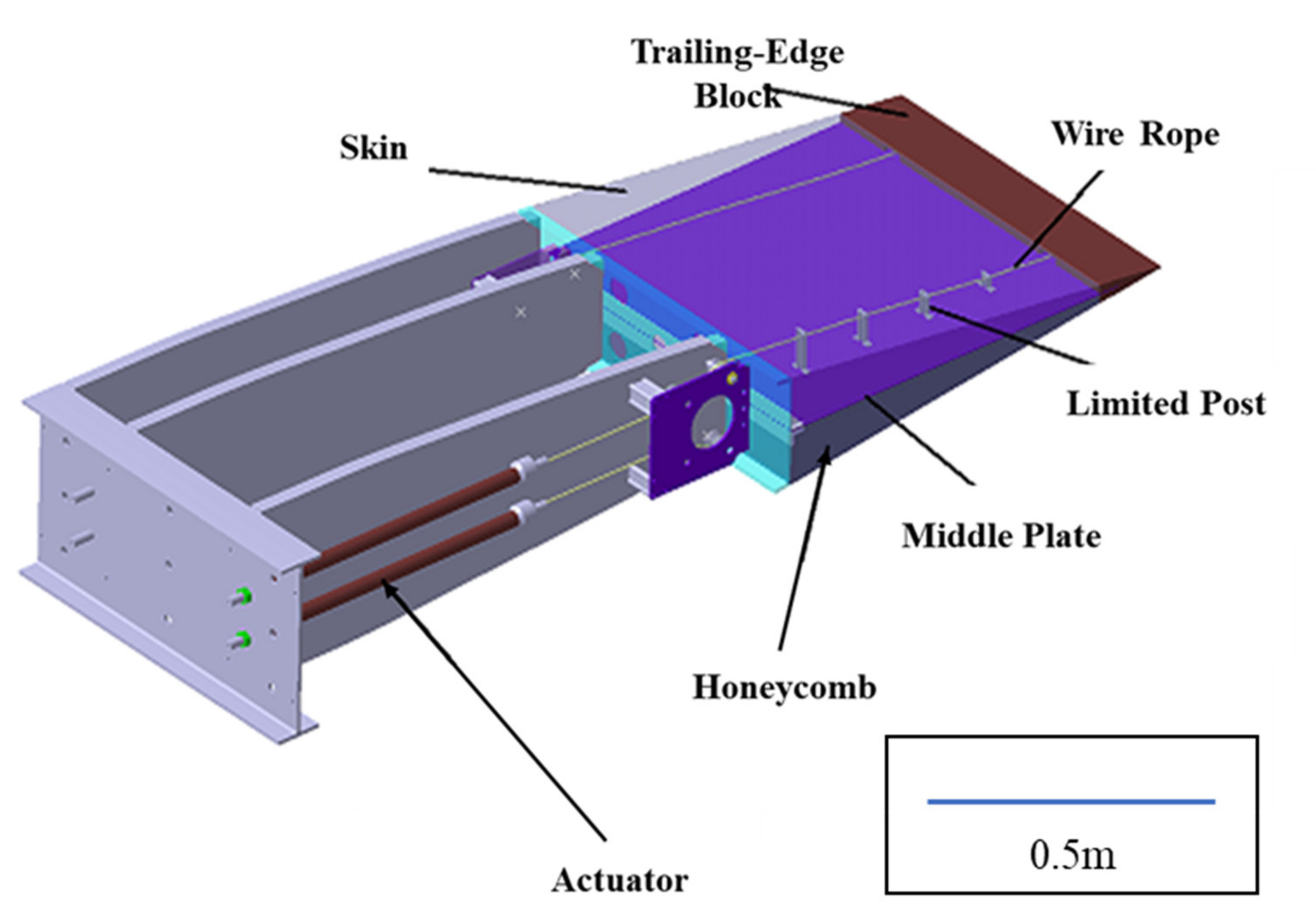
The flexible trailing edge structure shown in Figure 1 consists of the following parts: the composite middle plate, the flexible skin, the flexible honeycomb, the limited post, the wire rope and the trailing edge block. The wire rope is connected to the pneumatic muscle actuators, which is used to produce the activation forces. With the increase in internal pressure, the pneumatic muscle actuators contract to drive the FTE. The limited posts are used to constrain the wire rope’s movement to prevent damage to the flexible skin in the large deformation. The baseline airfoil is NACA0012. The length of the test model’s chord is 2000 mm. The length of span is 500 mm. The length of FTE in chord direction is 600 mm.
2.1.1. Actuator Model
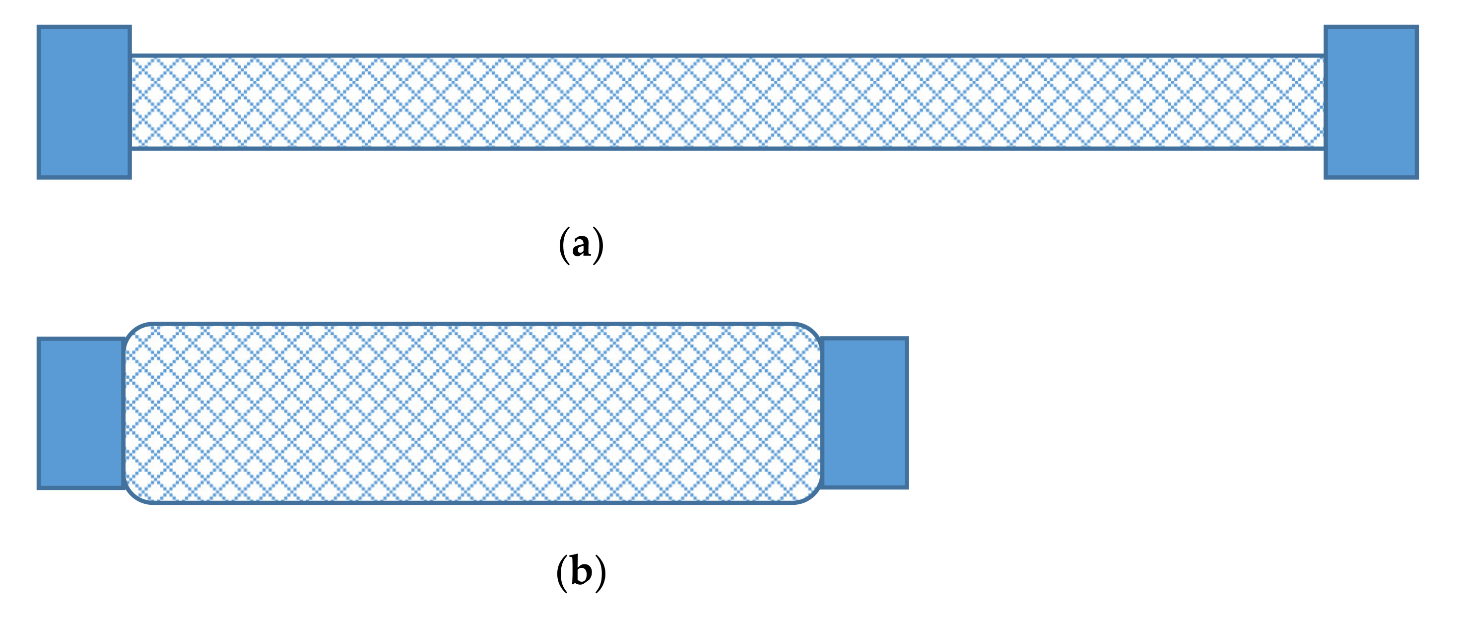
The actuation concept of pneumatic artificial muscles is shown in Figure 2. As the actuator is filled with air, it expands in the radial direction. A reduction in the overall length of the actuator is produced. In order to simplify the actuation model, surrogate model is established based on the experiment data to estimate the driving pressure. Quadratic response surface model is used here to validate the pressure result of simulation with the experiment data. The driving pressure is estimated based on the actuation force and contraction of the pneumatic artificial muscle actuator. These two items can be obtained by the FE model of FTE.
2.1.2. Wire-Pulley Transmission Model
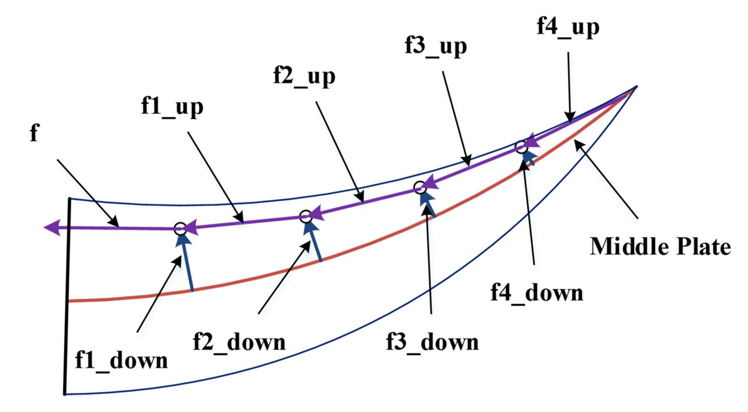
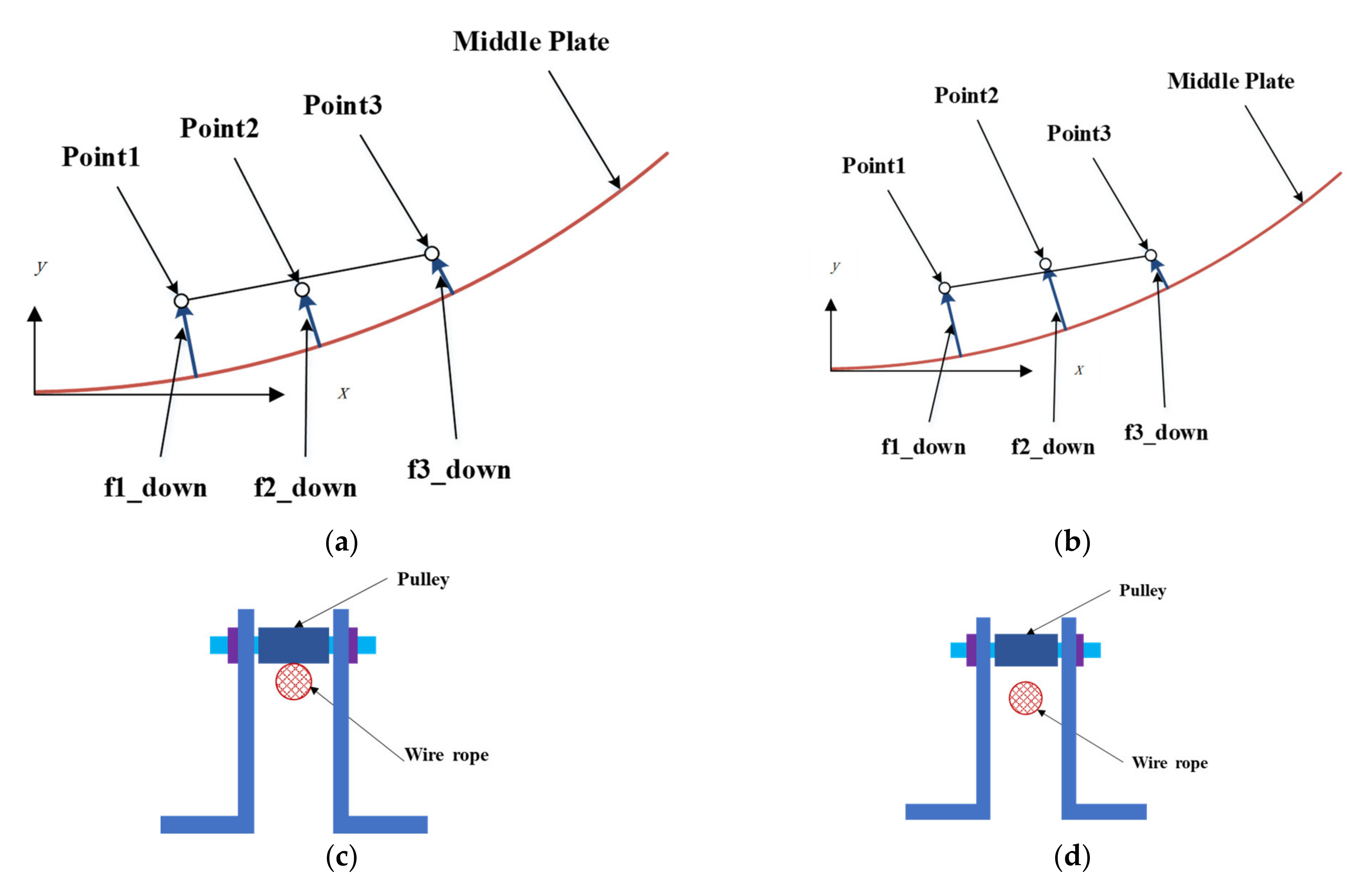
The limited posts, wire rope and the contact between them are not easy to establish in FE model. In this paper, MATLAB code is used to calculate the directions of internal forces (f1_up, f2_up, f3_up, f4_up) of wire rope as shown in Figure 3. The limited posts and wire rope are substituted by the internal forces (f1_down, f2_down, f3_down, f4_down). If the friction between the rope and the pulley is neglectful, the magnitude of the internal forces of wire rope is equal to the magnitude of activation force produced by the pneumatic muscle actuators. The equivalent forces (f1_down, f2_down, f3_down, f4_down) applied to the middle plate can be calculated as shown in Figure 4. Relative position relationship between the rope and pulley is as follows: (a) f2_down exists; (b) f2_ down does not exist; (c) f2_down exists; (d) f2_down does not exist. By calculating the relative position relationship between the rope and limited posts, the MATLAB code can be used to determine the existence of the corresponding equivalent force., as shown in Figure 4. Relative position relationship between the rope and pulley is as follows: (a) f2_down exists; (b) f2_ down does not exist; (c) f2_down exists; (d) f2_down does not exist. If point 2 is in the upside of the line connected by point 1 and point2, f2_down exists. If point 2 is in the downside of the line connected by point 1 and point2, f2_down does not exist.
2.1.3. Flexible Trailing Edge Model
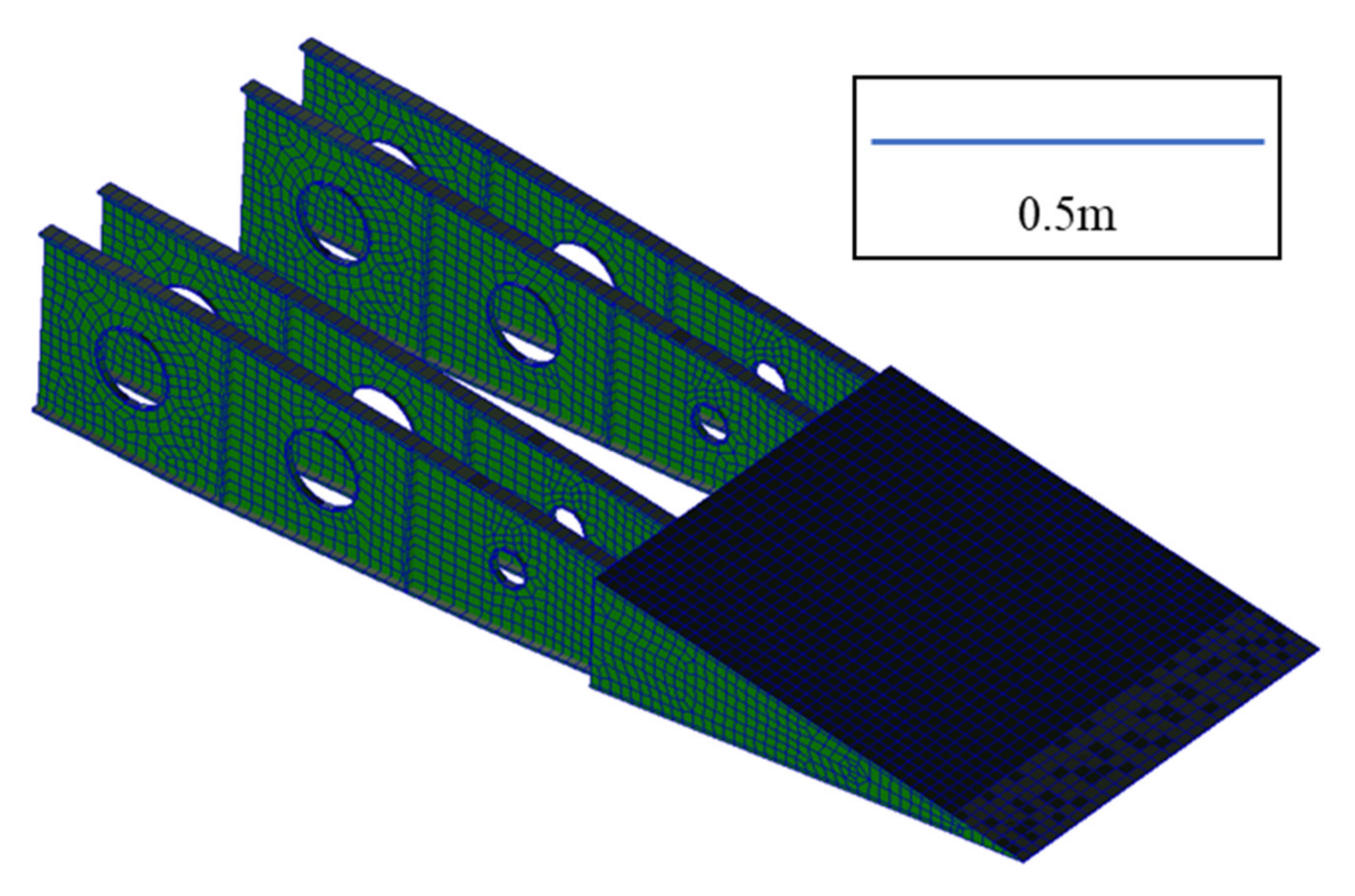
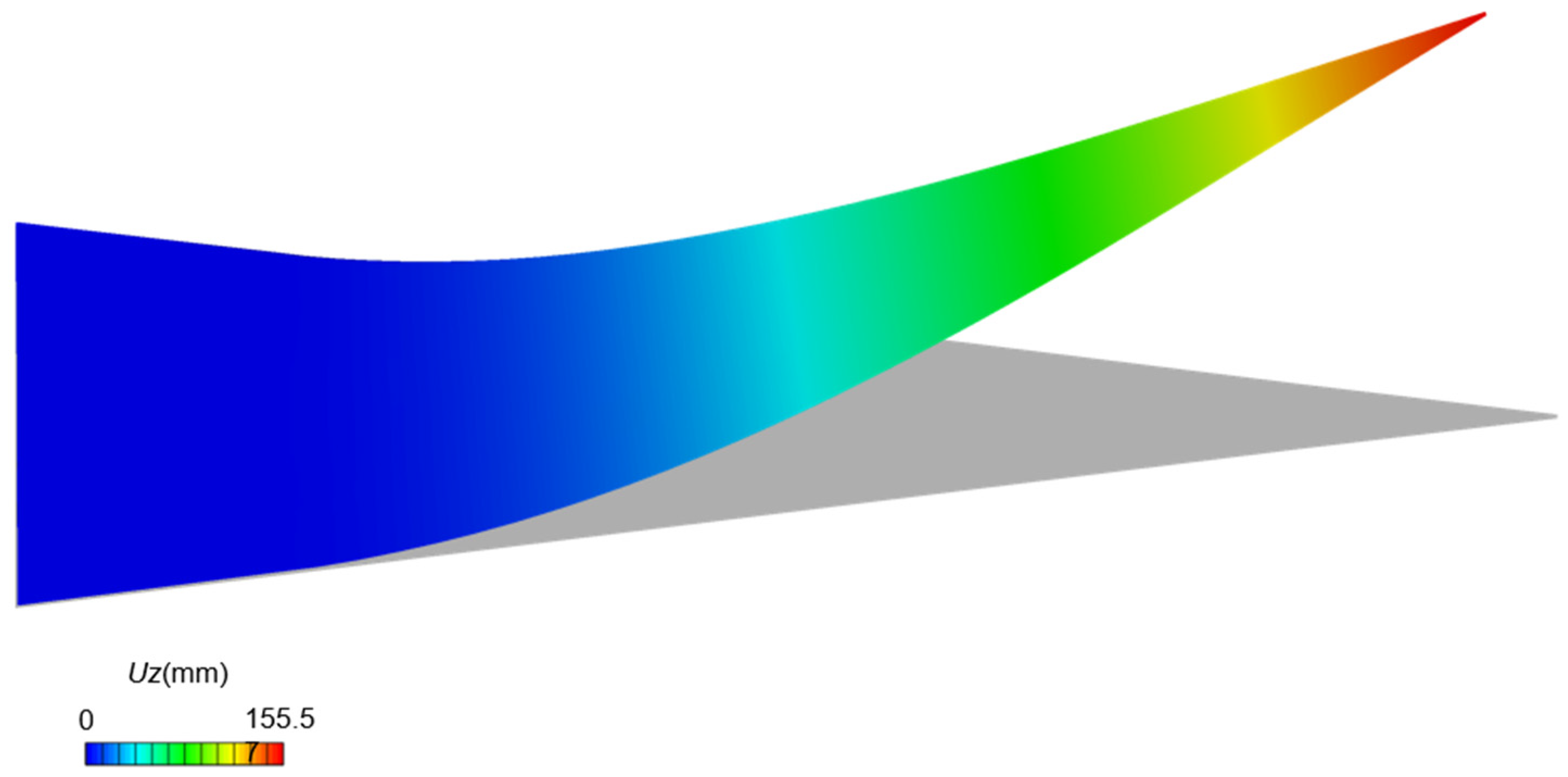
An FE model is established according to the test model, as shown in Figure 5. The FE model contains the following parts: the ribs, the composite middle plate, the flexible skin, the flexible honeycomb, and the trailing edge block. The ribs, the middle plate, the flexible skin are established using shell element. The minimum grid size is 14 mm. The trailing edge block and the flexible honeycomb are established using 3D element. The minimum grid size is 1.5 mm. The skin is made of silicone. The properties of flexible honeycomb with overlying elastomer are shown in Table 1 [17]. The material of middle plate is carbon fiber composite. The unidirectional lamina material properties are listed in Table 2. The fiber direction is the same as the chord direction. The thickness is 2 mm. The elastic modulus of silicone skin is 2.14 MPa, and Poisson’s ratio 0.45. The elastic modulus of aluminum middle plate is 72 GPa, and Poisson’s ratio 0.33. Figure 6 shows the deformation shape of the FE model when the deflection angle is 15°. The deflection angle is defined as the tip displacement divided by the length of flexible trailing edge in chord direction.
2.1.4. Physical Flexible Trailing Edge
A physical morphing wing model with FTE is manufactured using honeycomb structure. Experiment is conducted to verify the FE model. The FTE deflection is measured based on binocular vision. The test model is shown in Figure 7. The FTE is placed vertically so as to reduce the effect of gravity. Some markers are placed on the edge of the FTE to obtain the 3D coordinates of them. By calculating the distance of the markers from the two cameras, the 3D coordinates of the markers can be obtained. By obtaining all the markers’ 3D coordinates, the original and deformed shape of the FTE can be described.
The measurement method based on binocular vision principle is a non-contact and multi-point measurement technology. Firstly stick the markers on the flexible trailing edge. Based on the coordinates of the markers displacement of expected points on the FTE, deformation shape of the trailing edge can be calculated. Both cross and speckle pattern markers are used in the test. The binocular vision system is composed of two CMOS industrial cameras, tripod with a bar, and VIC-3D software, as shown in Figure 8. The two cameras are Gazelle GZL-CL-41C6M series by Point Grey Company, which are used to capture the flexible trailing edge synchronously from different perspectives. The bar on the tripod is used to clamp the cameras, and it can be adjusted in three directions. The VIC-3D software is used to process the captured pictures to obtain the coordinates of the markers. Binocular vision measurement includes camera calibration, image acquisition and processing, etc. Calibration is the process of solving camera parameters, which is used to determine the relationship between the 3D geometric position of the space and the corresponding points in the image [31]. Camera calibration must be carried out before test, as the results affect the accuracy of binocular vision measurement directly. Circular point array calibration target is used to calibrate the two cameras in this paper. Computer vision techniques including feature extraction and 3D reconstruction are used to process image pairs. Both cameras calibration and image processing are completed in the VIC-3D software, in which the 3D coordinates of markers can be calculated. In order to analyze the dynamic deformation of the FTE, images are captured by two cameras with an interval of 0.02 s. The measurement accuracy of the binocular vision system is 0.1 mm.
The measurement accuracy of the binocular vision system can be validated by measuring the known distance between markers as shown in Figure 8. The given distances between markers are measured by millimeter scale. The distances measured by the binocular vision system is compared with the known distance, as shown in Table 2. It can be seen that the errors are within 0.1 mm, which indicates that the measurement accuracy of the binocular vision system is 0.1 mm.
2.1.5. Validation of the Structure Model
The relationship between the driving pressure and deflection angle should be validated. Figure 8 shows the simulation result and test data of the relationship between driving pressure and deflection angle. Good agreement is achieved. Before driving pressure reaches 0.045 MPa, the displacement is zero. This is because under the pressure magnitude, the actuator could not produce any actuation force. With the increase in driving pressure magnitude, the deflection angle increases. The relationship between them is nearly linear. When the driving pressure exceeds 0.2 MPa, the relationship between them is obviously nonlinear. This is due to the nonlinearity between the wire movement (or actuator contraction) and the deflection angle.
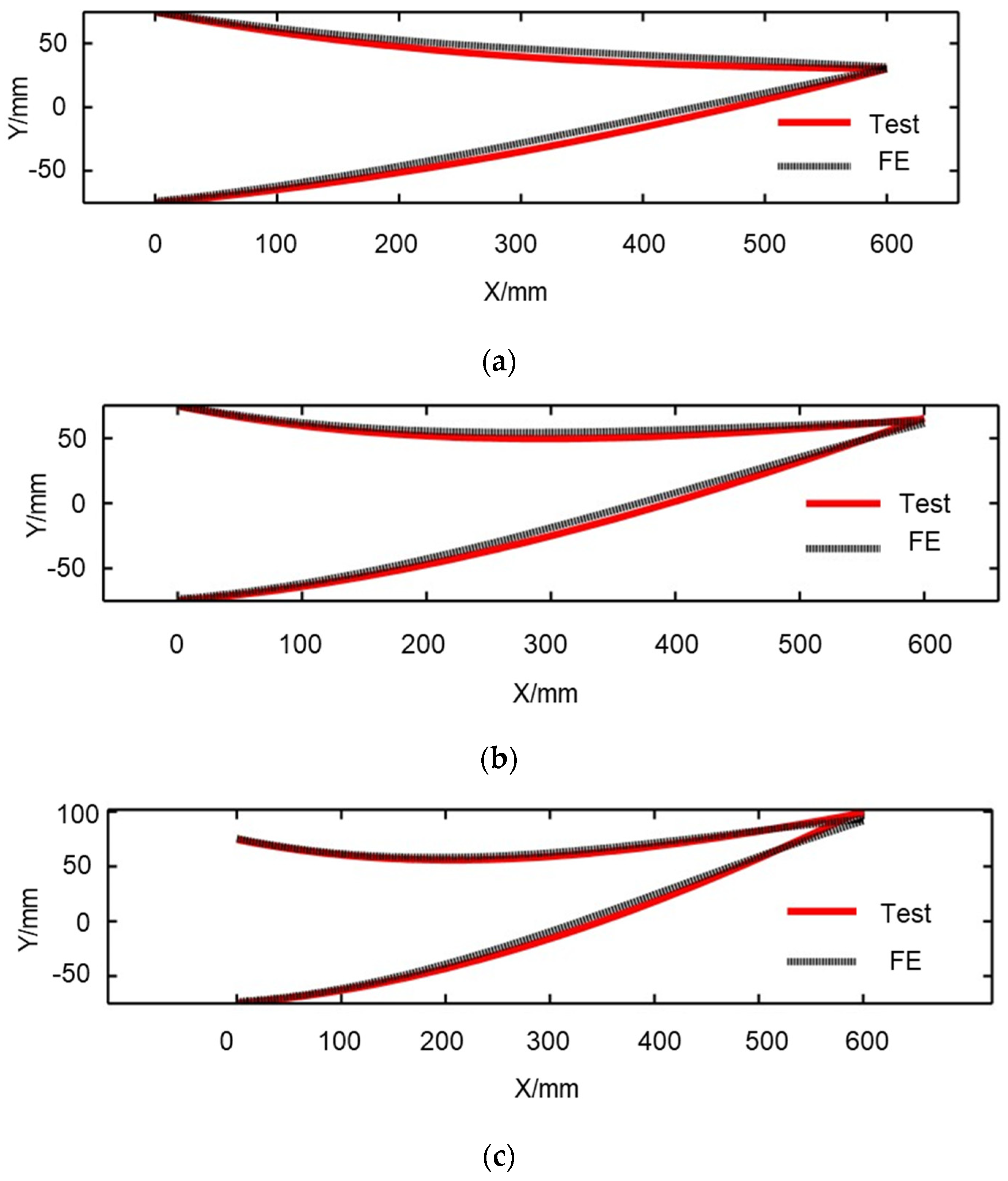
The deformation shapes of the FE model should also be validated with the measured shapes. Figure 9 shows the comparation of the simulated and measured shape under different deflection angles. The agreement of the FE model and test model is also quite good.
2.2. Static Aeroelastic Analysis
2.2.1. Aerodynamic Model
The aerodynamic pressure distribution acting on the structure is calculated using the XFOIL, the well-known free-licensed aerodynamic analysis code written by Mark Drela in 1986 [32]. Compared to other CFD solvers, XFOIL is faster and has been used in a series of works on morphing airfoils. Cody et al. [33] used XFOIL to perform fast and relatively accurate 2D steady-flow simulations of different morphed configurations using a camber-controlled morphed wing for maneuvering. Fincham et al. [34] adopted XFOIL as the source of aerodynamic predictions. It was found that the performance of the morphing aerofoil was nearly as good as a hypothetical aerofoil. XFOIL is compared against the open-source CFD solver OpenFOAM by Benjamin et al. [35]. XFOIL was found to provide very similar aerodynamic performance predictions to OpenFOAM, but at a fraction of the computational cost incurred by the CFD solver. Moreover, XFOIL is easy to integrate into MATLAB, and so provides an ideal solution for the static aeroelastic analysis. The aerodynamic conditions are as follows: Mach number is 0.1, Reynolds number is 5.2 × 10⁶.
2.2.2. Static Aeroelastic Analysis
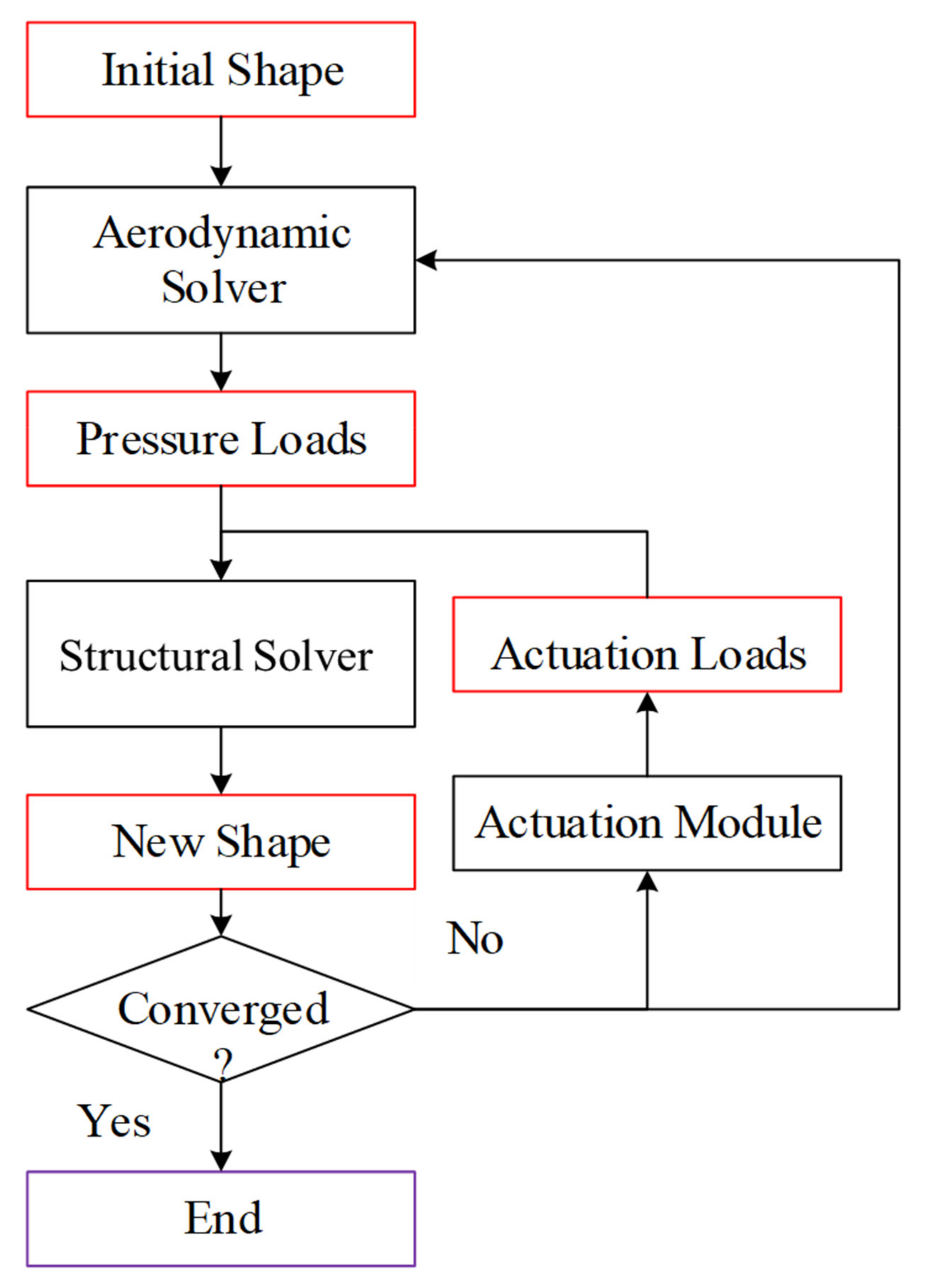
The static aeroelastic algorithm shown in Figure 10 is as follows. The static aeroelastic model couples a 3D FE model with a 2D viscous XFOIL panel code model. The FE and XFOIL simulations run separately with the solution of one passed to the other using a fully automated MATLAB script. Firstly calculate the pressure loads of the initial airfoil using XFOIL. Secondly distribute the pressure loads into the structural model, calculate the FE model using NASTRAN to get a new shape of the model. Thirdly if the lift coefficient, drag coefficient and displacement differences between the current step and the previous step are less than 1% of the total value, it is concluded that the static aeroelastic analysis is convergent. If not, extract the shape of the model in the previous step from NASTRAN’s result file. Import the shape data into MATLAB, and then call XFOIL to calculate the pressure loads of the shape. Based on the shape of the previous step, calculate the new equivalent forces (actuation loads) applied to the middle plate. Definition of lift coefficient is as follows:
where L is the lift, ρ is the air density, v is the velocity, S is the wing area.
Definition of lift coefficient is as follows:
where D is the drag, ρ is the air density, v is the velocity, S is the wing area.
2.2.3. Aerodynamic Load Transformation
The shape of the model in the previous step can be extracted from NASTRAN’s result file. Through the extracted shape data, the pressure loads can be obtained using XFOIL. However the aerodynamic coordinates and the structural coordinates are different, aerodynamic loads cannot be applied to the FE model directly, they need to be converted from the aerodynamic coordinate to the structural coordinate. The aerodynamic displacements that correspond to any linear combination of the structural displacements can be determined by the following:
where is the matrix corresponding to the evaluation of the interpolation at the aerodynamic nodes. is the interpolation matrix based on the radial basis function approach. is the coupling matrix that transforms the aerodynamic displacements to the structural ones.
Based on the principle of virtual work, we can get the following expression:
where is the aerodynamic load on the structural nodes, is the aerodynamic load on the aerodynamic nodes. is the matrix that we need to transform aerodynamic load from aerodynamic nodes to the structural ones.
where is the dimension of Euclidean space. Here, due to the number of coordinates, the value of here for 3D FE model is 3. is the aerodynamic nodes’ number.
The symmetric matrix can be written as follows:
where the following applies:
where . is the structural nodes’ number.
where .
3. Results and Discussion
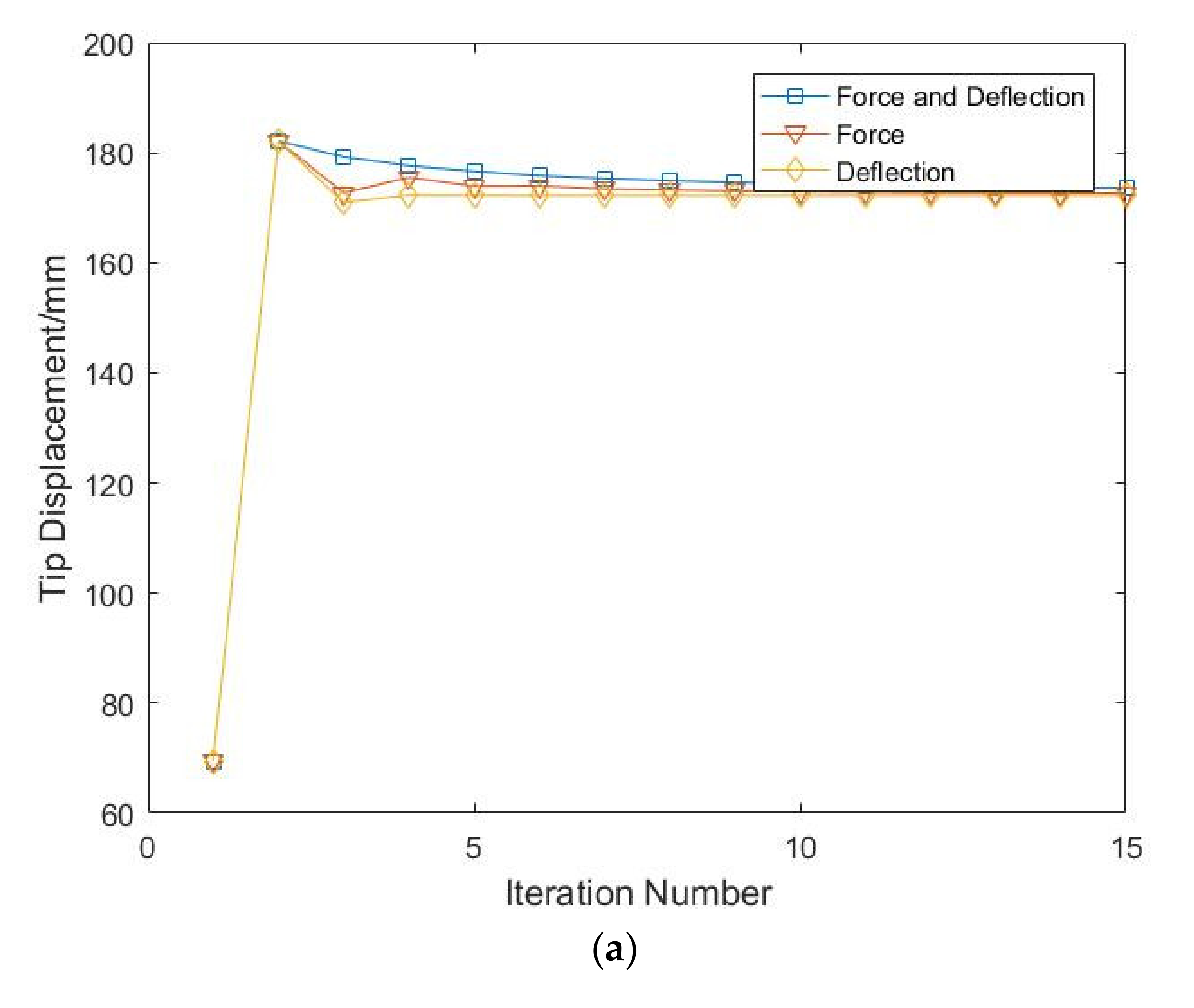
A fixed relaxation parameter is adopted in the static aeroelastic analysis. Relaxation parameters work by adding numerical damping to the solution, whereby the solution is only partially moved toward the solution predicted for the next iteration. In this way, the change during the iteration is reduced, and the tendency to experience fluctuating solutions of increasing divergence is tempered. If properly formulated, relaxation parameters do not change the value of the final converged solution, although they can decrease the speed of convergence. A simple form of a fixed relaxation parameter is as follows:
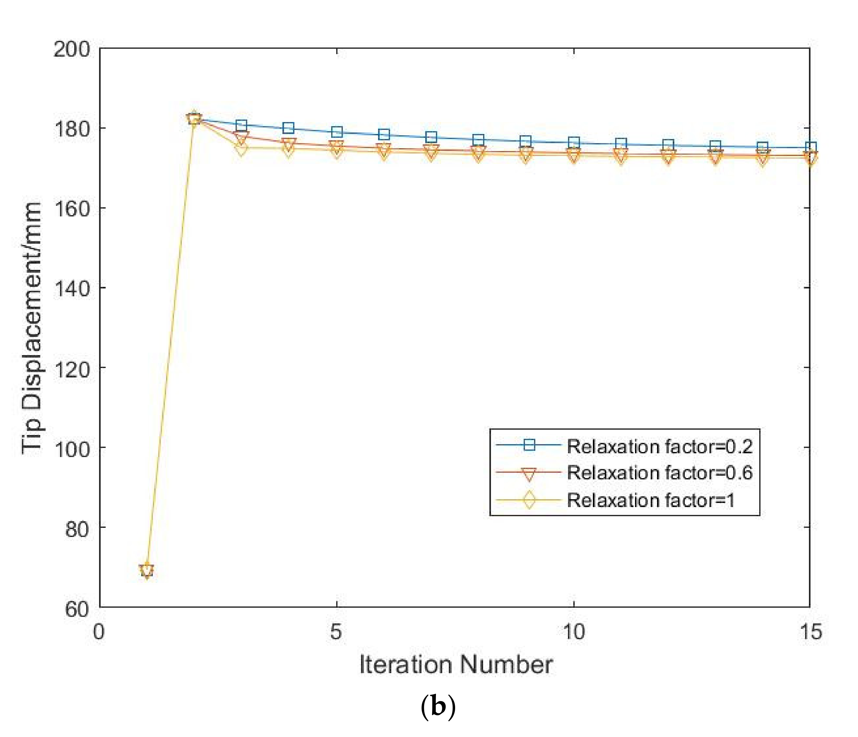
where the fixed relaxation parameter is a constant value, tuned for the static aeroelastic analysis, and is the estimated solution for the next iteration. A value of close to zero will lead to a very slow, but stable, convergence, whereas values close to one will reduce the relaxation effect, increasing the risk of instability.
Typically, two coupled components (deflection, force) can be found in the static aeroelastic analysis. As shown in Figure 11a, applying a relaxation parameter to force is sufficient to stabilize the convergence. Relaxing the deflection produces the best result, providing a quick and stable approach to the converged solution. As shown in Figure 11b, the closer the value of is to one, the faster the convergence rate is. However, this would also increase the risk of instability. Therefore, the selected value of is 0.4.
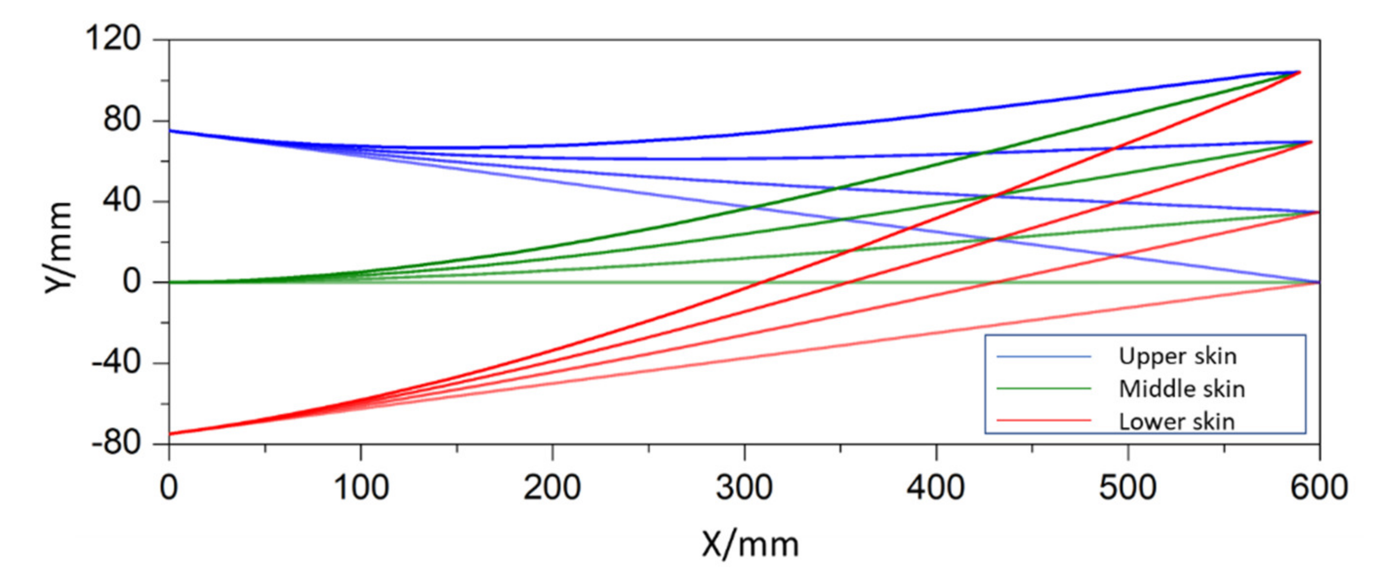
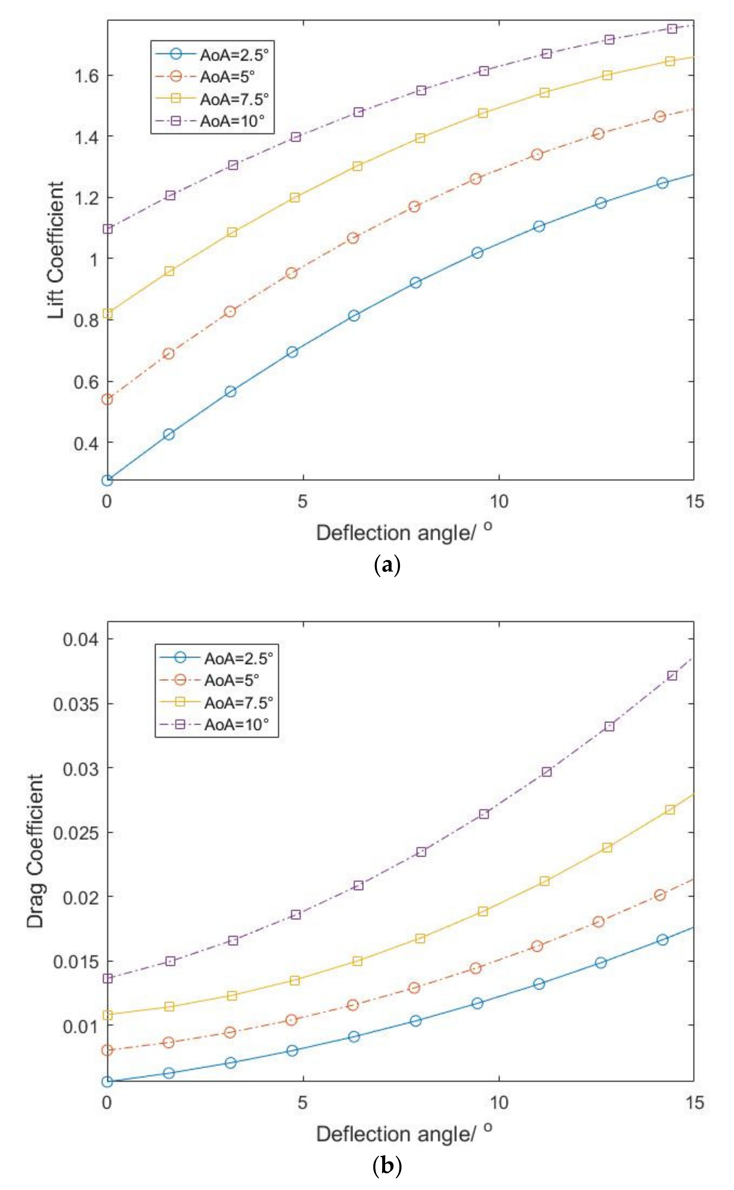
As the driving pressure increases, the deflection angle increases. The position of middle plate, and upper and lower skins under different pressures is shown in Figure 12. The relationship between the aerodynamic coefficients and deflection angle is shown in Figure 13. It shows that as the angle of attack increases, the magnitude of the lift coefficient increases less. However, the magnitude of the drag coefficient increases more with the increase in the deflection angle.
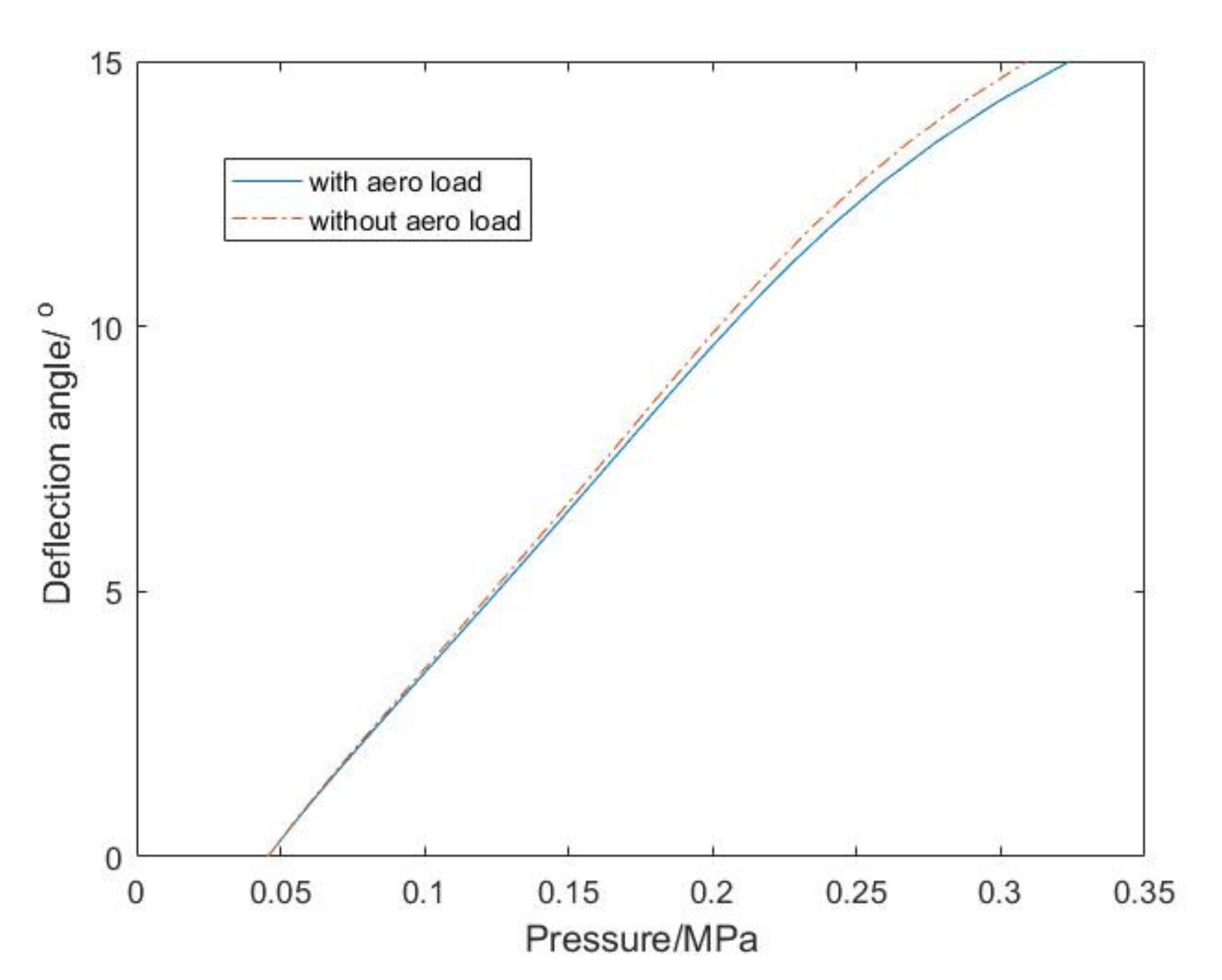
Compared to a traditional control surface, FTE needs to bear the structure stiffness besides the aerodynamic force. Figure 14 shows the relationship between the driving pressure and deflection angle, including the actuation force results for the same geometry configuration, but with no applied aerodynamic loading. This provides insight into the relative stiffness of the structural and aerodynamic loads. For the fairly low-speed condition studied here, the aerodynamic pressure on the trailing edge is quite low, and most of the driving pressure required to deflect the model is from the structural stiffness.
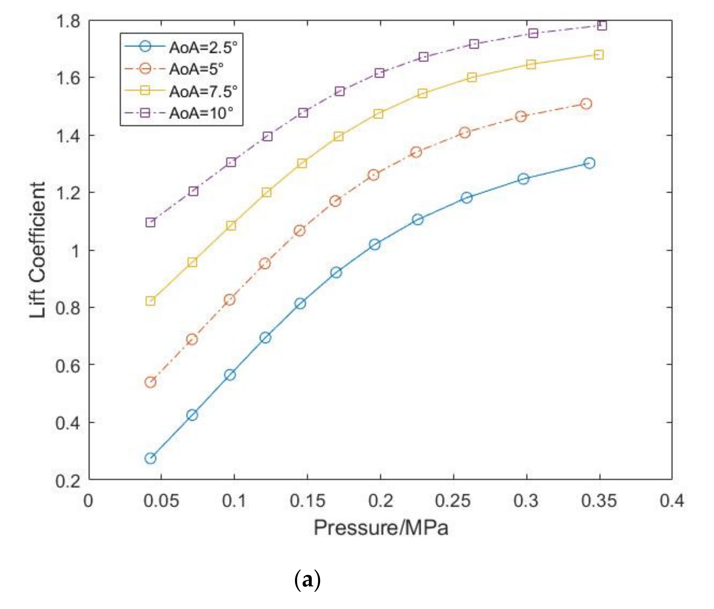
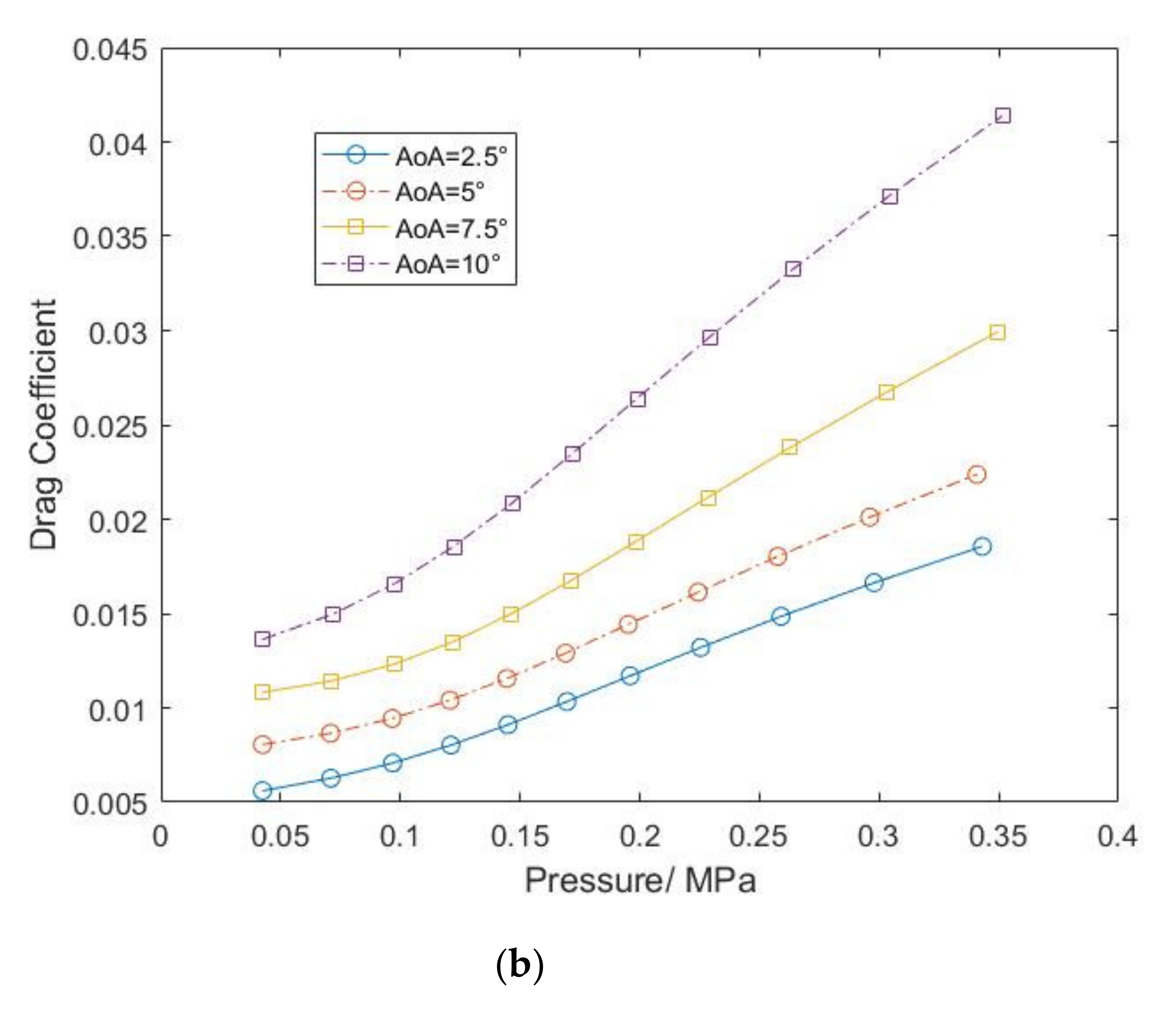
In order to predict the pressure needed for a given lift coefficient, the relationship between the actuation force and aerodynamic coefficients is investigated. Figure 15a shows the relationship between the driving pressure and lift coefficient. Figure 15b shows the relationship between the driving pressure and drag coefficient. With the increase in the driving pressure, the magnitude of the lift coefficient increases less. However, the magnitude of the drag coefficient increases more with the increase in pressure under 0.2 MPa. When the driving pressure exceeds 0.2 MPa, the relationship between them is nearly linear. This is because a nonlinear relationship can be found between the pressure and deflection angle.
4. Conclusions
In this paper, an investigation of a morphing trailing edge’s static aeroelastic characteristics is conducted. Flight efficiency could be improved by using FTE because of its high aerodynamic efficiency. The dynamic characteristics of FTE will be investigated in future work.
The actuator model is established based on the quadratic response surface method. The wire-pulley transmission model is built to identify the existence of equivalent forces, and produce the equivalent forces as the substitute of actuation force. A finite element model of the morphing trailing edge is established, which is validated by the test data. A nonlinear relationship is found between the driving pressure and deflection angle. This is due to the nonlinear relationship between the actuation force and driving pressure.
The results show that the pressure needed to bear the structural stiffness is much larger than that of the aerodynamic loads, when the Mach number is 0.1. With the increase in pressure, the magnitude of the lift coefficient increases less. However, the magnitude of the drag coefficient increases more with the increase in pressure under 0.2 MPa. When the driving pressure exceeds 0.2 MPa, the relationship between them is nearly linear.
Author Contributions
Conceptualization, S.Z., D.L. and J.Z.; methodology, S.Z., E.S.; validation, S.Z.; formal analysis, S.Z., J.Z.; investigation, D.L., E.S.; resources, S.Z., D.L.; data curation, S.Z., E.S.; writing—original draft preparation, S.Z.; writing—review and editing, S.Z., J.Z.; visualization, S.Z., J.Z.; supervision, S.Z., J.Z.; project administration, S.Z., D.L. and J.Z. All authors have read and agreed to the published version of the manuscript.
Funding
The research was funded in part by the National Natural Science Foundation of China (Grant No. 11402014; Grant No. 11572023), and in part by the National Research Project “Variable Camber Wing Technology(VCAN)” of China.
Institutional Review Board Statement
Not applicable.
Informed Consent Statement
Not applicable.
Data Availability Statement
Not applicable.
Conflicts of Interest
The authors declare no conflict of interest.
References
- Li, D.; Zhao, S.; Da Ronch, A.; Xiang, J.; Drofelnik, J.; Li, Y.; Zhang, L.; Wu, Y.; Kintscher, M.; Monner, H.P.; et al. A review of modelling and analysis of morphing wings. Prog. Aerosp. Sci. 2018, 100, 46–62. [Google Scholar] [CrossRef] [Green Version]
- Ismail, N.; Zulkifli, A.; Abdullah, M.; Basri, M.H.; Abdullah, N.S. Optimization of aerodynamic efficiency for twist morphing MAV wing. Chin. J. Aeronaut. 2014, 27, 475–487. [Google Scholar] [CrossRef] [Green Version]
- Huang, R.; Qiu, Z. Transient aeroelastic responses and flutter analysis of a variable-span wing during the morphing process. Chin. J. Aeronaut. 2013, 26, 1430–1438. [Google Scholar] [CrossRef] [Green Version]
- Koreanschi, A.; Gabor, O.S.; Acotto, J.; Brianchon, G.; Portier, G.; Botez, R.M.; Manou, Y.; Mebarki, Y. Optimization and design of an aircraft’s morphing wing-tip demonstrator for drag reduction at low speed, Part I—Aerodynamic optimization using genetic, bee colony and gra-dient descent algorithms. Chin. J. Aeronaut. 2017, 30, 149–163. [Google Scholar] [CrossRef]
- Koreanschi, A.; Gabor, O.S.; Acotto, J.; Brianchon, G.; Portier, G.; Botez, R.M. Optimization and design of an aircraft’s morphing wing-tip demonstrator for drag reduction at low speeds, Part II-Experimental validation using Infra-Red transition measure-ment from Wind Tunnel tests. Chin. J. Aeronaut. 2017, 30, 164–174. [Google Scholar] [CrossRef]
- Li, D.; Liu, Q.; Wu, Y.; Xiang, J. Design and analysis of a morphing drag rudder on the aerodynamics, structural deformation, and the required actuating moment. J. Intell. Mater. Syst. Struct. 2018, 29, 1038–1049. [Google Scholar] [CrossRef]
- Kan, Z.; Li, D.; Xiang, J. Delaying stall of morphing wing by periodic trailing-edge deflection. Chin. J. Aeronaut. 2020, 33, 493–500. [Google Scholar] [CrossRef]
- Xiang, J.; Liu, K.; Li, D.; Cheng, C.; Sha, E. Unsteady aerodynamic characteristics of a morphing wing. Aircr. Eng. Aerosp. Technol. 2018, 91, 1–9. [Google Scholar] [CrossRef]
- Li, D.; Guo, S.; Aburass, T.O.; Yang, D.; Xiang, J. Active control design for an unmanned air vehicle with a morphing wing. Aircr. Eng. Aerosp. Technol. 2016, 88, 168–177. [Google Scholar] [CrossRef]
- Li, D.; Guo, S.; Xiang, J. Modeling and nonlinear aeroelastic analysis of a wing with morphing trailing edge. Proc. Inst. Mech. Eng. Part G J. Aerosp. Eng. 2012, 227, 619–631. [Google Scholar] [CrossRef]
- Li, D.; Guo, S.; He, Y.; Xiang, J. Nonlinear aeroelastic analysis of a morphing flap. Int. J. Bifurc. Chaos 2012, 22, 1250099. [Google Scholar] [CrossRef]
- Woods, B.K.; Bilgen, O.; Friswell, M.I. Wind Tunnel Testing of the Fishbone Active Camber Morphing Concept. J. Int. Mat. Syst. Str. 2014, 5, 772–785. [Google Scholar] [CrossRef]
- Chen, Q.; Bai, P.; Yin, W.; Leng, J.; Zhan, H.; Liu, Z. Analysis on the aerodynamic characteristics of variable camber airfoils with continuous smooth morphing trailing edge. Acta Phys. 2010, 28, 46–53. [Google Scholar]
- Woods, B.K.S.; Dayyani, I.; Friswell, M. Fluid/Structure-Interaction Analysis of the Fish-Bone-Active-Camber Morphing Concept. J. Aircr. 2015, 52, 307–319. [Google Scholar] [CrossRef] [Green Version]
- Yokozeki, T.; Sugiura, A.; Hirano, Y. Development of Variable Camber Morphing Airfoil Using Corrugated Structure. J. Aircr. 2014, 51, 1023–1029. [Google Scholar] [CrossRef] [Green Version]
- Airoldi, A.; Crespi, M.; Quaranti, G.; Sala, G. Design of a Morphing Airfoil with Composite Chiral Structure. J. Aircr. 2012, 49, 1008–1019. [Google Scholar] [CrossRef]
- Zhang, P.; Zhou, L.; Cheng, W.; Qiu, T. Conceptual Design and Experimental Demonstration of a Distributedly Actuated Morphing Wing. J. Aircr. 2015, 52, 452–461. [Google Scholar] [CrossRef]
- Xie, D.; Ma, Z.; Liu, J.; Zuo, S. Pneumatic Artificial Muscle Based on Novel Winding Method. Actuators 2021, 10, 100. [Google Scholar] [CrossRef]
- Cao, Y.; Fu, Z.; Zhang, M.; Huang, J. Extended-State-Observer-Based Super Twisting Control for Pneumatic Muscle Actuators. Actuators 2021, 10, 35. [Google Scholar] [CrossRef]
- Zhao, W.; Song, A. Active Motion Control of a Knee Exoskeleton Driven by Antagonistic Pneumatic Muscle Actuators. Actuators 2020, 9, 134. [Google Scholar] [CrossRef]
- Yin, W.; Liu, L.; Chen, Y.; Leng, J. Variable camber wing based on pneumatic artificial muscles. In Proceedings of the Second International Conference on Smart Materials and Nanotechnology in Engineering, Weihai, China, 8–11 July 2009. [Google Scholar]
- Barbarino, S.; Pecora, R.; Lecce, L.; Concilio, A.; Ameduri, S.; Calvi, E. A Novel SMA-based Concept for Airfoil Structural Morphing. J. Mater. Eng. Perform. 2009, 18, 696–705. [Google Scholar] [CrossRef]
- Bae, J.S.; Kyong, N.H.; Seigler, T.M. Aeroelastic Considerations on Shape Control of an Adaptive Wing. J. Int. Mat. Syst. Str. 2005, 16, 1051–1056. [Google Scholar] [CrossRef]
- Campanile, L.F.; Anders, S. Aerodynamic and aeroelastic amplification in adaptive belt-rib airfoils. Aerosp. Sci. Technol. 2005, 9, 55–63. [Google Scholar] [CrossRef]
- Bilgen, O.; Flores, E.I.S.; Friswell, M.I. Optimization of Surface-Actuated Piezocomposite Variable-Camber Morphing Wings. In Smart Materials, Adaptive Structures and Intelligent Systems, Proceedings of the ASME 2011 Conference on Smart Materials, Adaptive Structures and Intelligent Systems, Scottsdale, AZ, USA, 18–21 September 2011; Adaptive Structures and Intelligent Systems American Society of Mechanical Engineers: New York, NY, USA, 2011; pp. 315–322. [Google Scholar]
- Daynes, S.; Weaver, P.M. Morphing Blade Fluid-Structure Interaction. In Proceedings of the 53rd AIAA Structures, Structural Dynamics, and Materials Conference, Honolulu, HI, USA, 23–26 April 2012; pp. 1–15. [Google Scholar]
- Botez, R.M.; Koreanschi, A.; Gabor, O.S. Numerical and experimental transition results evaluation for a morphing wing and aileron system. Aeronaut. J. 2018, 122, 747–784. [Google Scholar] [CrossRef]
- Communier, D.; Botez, R.; Wong, T. Experimental validation of a new morphing trailing edge system using Price—Païdoussis wind tunnel tests. Chin. J. Aeronaut. 2019, 32, 1353–1366. [Google Scholar] [CrossRef]
- Yerkes, N.; Wereley, N. Pneumatic Artificial Muscle Activation for Trailing Edge Flaps. In Proceedings of the 46th AIAA Aerospace Sciences Meeting and Exhibit, Reno, NV, USA, 7–10 January 2008; American Institute of Aeronautics and Astronautics: Reston, VA, USA, 2008; pp. 1–10. [Google Scholar]
- Woods, B.K.S. Pneumatic Artificial Muscle Driven Trailing Edge Flaps for Active Rotors[M]; University of Maryland: College Park, MD, USA, 2012. [Google Scholar]
- Bradski, G.; Kaehler, A. Learning OpenCV: Computer Vision in C++ with the OpenCV Library; O’Reilly Media, Inc.: Sebastopol, CA, USA, 2013. [Google Scholar]
- Drela, M. XFOIL: An Analysis and Design System of Low Reynolds Number Aerofoils. Low Reynolds Number Aerodyn. 1989, 54, 1–12. [Google Scholar]
- Cody, L.; Kelly, C.; Shaaban, A. Use of XFOIL in design of camber-controlled morphing UAVs. Comput. Appl. Eng. Educ. 2012, 20, 673–680. [Google Scholar]
- Woods, B.; Fincham, J.H.S.; Friswell, M.I. Aerodynamic modelling of the fish bone active camber morphing concept. In Proceedings of the RAeS Applied Aerodynamics Conference 2014, Bristol, UK, 22–24 July 2014. [Google Scholar]
- Fincham, J.H.S.; Friswell, M.I. Aerodynamic optimisation of a camber morphing aerofoil. Aerosp. Sci. Technol. 2015, 43, 245–255. [Google Scholar] [CrossRef] [Green Version]
Figure 1.
Flexible trailing edge structure.

Figure 2.
Actuation concept of pneumatic artificial muscles: (a) initial state; (b) air pressured state.
Figure 2.
Actuation concept of pneumatic artificial muscles: (a) initial state; (b) air pressured state.

Figure 3.
Equivalent model of driving force.

Figure 4.
Relative position relationship between the rope and pulley: (a) f2_down exists; (b) f2_ down does not exist; (c) f2_down exists; (d) f2_down does not exist.
Figure 4.
Relative position relationship between the rope and pulley: (a) f2_down exists; (b) f2_ down does not exist; (c) f2_down exists; (d) f2_down does not exist.

Figure 5.
3D FE model of flexible trailing edge model.

Figure 6.
Deformation shape of FE model.

Figure 7.
Binocular vision test.

Figure 8.
Driving pressure vs. deflection angle.

Figure 9.
Simulated and measured shape: (a) deflection angle is 3°; (b) deflection angle is 6°; (c) deflection angle is 9°.
Figure 9.
Simulated and measured shape: (a) deflection angle is 3°; (b) deflection angle is 6°; (c) deflection angle is 9°.

Figure 10.
Static aeroelastic analysis algorithm schematic.

Figure 11.
Application of fixed relaxation parameter to various system components: (a) relaxing factor with and without force or deflection; (b) the influence of relaxation factor on the convergence rate.
Figure 11.
Application of fixed relaxation parameter to various system components: (a) relaxing factor with and without force or deflection; (b) the influence of relaxation factor on the convergence rate.


Figure 12.
Position of middle plate, and upper and lower skins under different pressures.

Figure 13.
Deflection angle vs. aerodynamic coefficients: (a) deflection angle vs. lift coefficient; (b) deflection angle vs. drag coefficient.
Figure 13.
Deflection angle vs. aerodynamic coefficients: (a) deflection angle vs. lift coefficient; (b) deflection angle vs. drag coefficient.

Figure 14.
Driving pressure vs. deflection angle under different conditions.

Figure 15.
Pressure vs. aerodynamic coefficients: (a) pressure vs. lift coefficient; (b) pressure vs. drag coefficient.
Figure 15.
Pressure vs. aerodynamic coefficients: (a) pressure vs. lift coefficient; (b) pressure vs. drag coefficient.


Table 1.
Properties of flexible honeycomb with overlying silicone skin.
| Parameters | (MPa) | (MPa) | (MPa) | (MPa) | (MPa) | (MPa) |
|---|---|---|---|---|---|---|
| Value | 0.094 | 0.181 | 0.58 | 1.88e3 | 228.46 | 270.66 |
Table 2.
Accuracy of binocular vision system.
| Item | By Binocular Vision/mm | Known/mm | Relative Error/% |
|---|---|---|---|
| Transverse | 100.087 | 100 | 0.087 |
| Longitudinal | 50.096 | 50 | 0.192 |
Publisher’s Note: MDPI stays neutral with regard to jurisdictional claims in published maps and institutional affiliations. |
© 2021 by the authors. Licensee MDPI, Basel, Switzerland. This article is an open access article distributed under the terms and conditions of the Creative Commons Attribution (CC BY) license (https://creativecommons.org/licenses/by/4.0/).
Share and Cite
MDPI and ACS Style
Zhao, S.; Li, D.; Zhou, J.; Sha, E. Numerical and Experimental Study of a Flexible Trailing Edge Driving by Pneumatic Muscle Actuators. Actuators 2021, 10, 142. https://doi.org/10.3390/act10070142
AMA Style
Zhao S, Li D, Zhou J, Sha E. Numerical and Experimental Study of a Flexible Trailing Edge Driving by Pneumatic Muscle Actuators. Actuators. 2021; 10(7):142. https://doi.org/10.3390/act10070142
Chicago/Turabian StyleZhao, Shiwei, Daochun Li, Jin Zhou, and Enlai Sha. 2021. "Numerical and Experimental Study of a Flexible Trailing Edge Driving by Pneumatic Muscle Actuators" Actuators 10, no. 7: 142. https://doi.org/10.3390/act10070142
Note that from the first issue of 2016, this journal uses article numbers instead of page numbers. See further details here.