Symbiotic Organism Search Algorithm with Multi-Group Quantum-Behavior Communication Scheme Applied in Wireless Sensor Networks

Abstract

The symbiotic organism search (SOS) algorithm is a promising meta-heuristic evolutionary algorithm. Its excellent quality of global optimization solution has aroused the interest of many researchers. In this work, we not only applied the strategy of multi-group communication and quantum behavior to the SOS algorithm, but also formed a novel global optimization algorithm called the MQSOS algorithm. It has speed and convergence ability and plays a good role in solving practical problems with multiple arguments. We also compared MQSOS with other intelligent algorithms under the CEC2013 large-scale optimization test suite, such as particle swarm optimization (PSO), parallel PSO (PPSO), adaptive PSO (APSO), QUasi-Affine TRansformation Evolutionary (QUATRE), and oppositional SOS (OSOS). The experimental results show that MQSOS algorithm had better performance than the other intelligent algorithms. In addition, we combined and optimized the DV-hop algorithm for node localization in wireless sensor networks, and also improved the DV-hop localization algorithm to achieve higher localization accuracy than some existing algorithms.

1. Introduction

In the past several decades, intelligent computing has developed rapidly. Researchers have evolved a variety of intelligent computing algorithms inspired by natural phenomena [1,2]. While conducting research, we often encounter complex problems that require the extreme value of a multivariate function to be found. The usual practice is to calculate the gradient of the function. When functions have higher dimensions or are relatively complex themselves, the gradient of the computational function will be very time consuming, and thus unable to complete tasks. Moreover, many problem functions are inseparable in real life, which limits the feasibility of the gradient calculation of correlated functions. The advent of computational intelligence provides a new way of thinking about the solution of these optimal solutions, thereby breaking the limitations of traditional methods for solving extreme values of functions that require low-dimensional differentiation. In this paper, we take the 28 unrestricted objective functions in CEC2013 [3,4,5] as an example to analyze and compare the newly proposed algorithms. Although the objective function has multiple constraints in the objective world, the performance of the objective function of the algorithm under unconstrained conditions plays a fundamental role in various optimization applications, which will then affect the performance and direction of the algorithm in a constrained objective function. Computational intelligence (CI) [6,7,8,9,10] not only deals with complex problems in real life (most notably the objective functions of uncertain or noisy problems [11]), it can also give calculation methods and solutions to solve these optimization problems. Evolutionary computation (EC) [12,13,14,15] is a branch of CI that provides an optimization method with evolutionary ideas. There are many branches in the CI field, such as computational learning theory (CLT), evolutionary computing, fuzzy logic (FL), artificial neural networks (ANNs), and quantum computing (QC). Swarm intelligence (SI) is one branch of evolutionary computing [16,17], including evolutionary algorithm (EAs), memetic calculation (MC), and so forth. EC encompasses a variety of optimization algorithms developed by researchers and various scholars. It is based on the inspiration and simulation of various natural phenomena in nature. The PSO algorithm is a classic intelligent algorithm inspired by the foraging behavior of birds. Many scholars have developed and improved on this basis to enhance the global optimization of PSO algorithms [18,19], with developments such as parallel PSO (PPSO) [20], adaptive PSO (APSO) [21], and so on. Differential evolution (DE) [5,5] is a stochastic model that simulates the evolution of organisms. It is an evolutionary algorithm that is preserved by individuals which adapt to the environment through repeated iterations. QUasi-Affine TRansformation Evolutionary (QUATRE) [22,23] is an algorithm based on the quasi-affine transformation in geometry. It overcomes the shortcoming of the DE algorithm where as the number of evolutionary iterations increases, the diversity of the population is reduced, and it converges to a local optimization point prematurely or the algorithm stagnates. The artificial bee colony (ABC) [24,25,26], ant colony optimization (ACO) [27], and cat group optimization algorithms (CSO) [28,29] also have similar functionalities.

Symbiotic organism search (SOS) [30,31] is a very promising meta-heuristic optimization algorithm with state-of-the-art global optimization ability. It uses the symbiotic relationship between two organisms in an ecosystem to survive, and cycles to find the optimal value of the objective function. In 2014, Cheng and Prayogo pioneered the algorithm. Subsequently, many researchers and scholars improved this algorithm [32,33]. For example, in 2019, Falguni Chakraborty, Debashis Nandi, and Provas Kumar Roy proposed oppositional SOS (OSOS) [30,34]. In order to further improve the global optimization ability of the SOS algorithm (including the optimal solution and convergence speed), this paper will integrate the quantum behavior [35,36] and the idea of multi-group optimization into the SOS algorithm, while drawing comparisons with the other algorithms mentioned in this paper. Experimental results indicate that the performance of the proposed MQSOS algorithm is superior to other algorithms.

Wireless network node positioning plays a very important role in wireless sensor networks (WSNs) [37,38,39,40], navigating, monitoring, and other applications [41,42]. According to whether the distance between nodes needs to be measured, the position can be divided into positioning based on the distance measurement and positioning not based on the distance measurement. On the basis of the deployment occasion, it can be divided into outdoor positioning and indoor positioning [43]. Common methods based on distance measurement include triangulation, trilateration, and maximum likelihood estimation [23,44,45]. Common ranging methods include DV-hop [46], RSSI [47,48], etc. The DV-hop-based positioning algorithm is simple and has high positioning accuracy, which has made the research results published in this area widely used in recent years. Many scholars have applied intelligent algorithms to wireless sensor network location algorithms based on distance measurement. The accuracy of positioning is being continuously improved. The combination of the MQSOS algorithm and the DV-hop algorithm to improve the performance of original DV-hop positioning is also proposed in this paper.

Section 2 of this paper briefly introduces the DV-hop algorithm and several EC algorithms such as native PSO, SOS, QUATRE, OSOS, and so on. Section 3 is dedicated to the newly proposed MQSOS algorithm and the algorithm MQSOS_DV-hop that is generated in combination with the DV-hop algorithm. Section 4 shows the experimental results under the CEC2013 test suite and compares the proposed method with other EC algorithms. At the same time, the improvement of the DV-hop algorithm by MQSOS and other CI algorithms is also compared. Finally, in Section 5, the corresponding conclusions are drawn based on the experimental results.

2. Related Works

2.1. Native PSO Algorithm

The PSO algorithm is a classic global optimization algorithm inspired by the foraging behavior of birds in nature, where the area where the birds forage is simulated as the range of the solution, the position of the bird is the position of the current particle, and the position of the food is the position of the global optimal solution. The specific process of the PSO algorithm is as follows. In the initial stage, the scope of the group search is set along with the critical value of the speed in the particle search process. The position of the randomly initialized group is $\mathbf{X}=\left[\begin{array}{c}{\mathbf{x}}_1,{\mathbf{x}}_2,\dots ,{\mathbf{x}}_{ps}\end{array}\right]$ and the speed is $\mathbf{V}=\left[\begin{array}{c}{\mathbf{v}}_1,{\mathbf{v}}_2,\dots ,{\mathbf{v}}_{ps}\end{array}\right]$.

$${\mathbf{x}}_i=(x_{i,1},x_{i,2},\dots ,x_{i,D}),$$

(1)

$${\mathbf{v}}_i=(v_{i,1},v_{i,2},\dots ,v_{i,D}),$$

(2)

where ${\mathbf{x}}_i$ and ${\mathbf{v}}_i$ represent the position and velocity of the ith particle in the population, D represents the dimension of the population, and $ps$ is the population size.

In the evolutionary stage, the iterative evolution of the population is continually carried out by Equations (3) and (4) until the conditions for the iterations to stop are met.

$${\mathbf{v}}_i^{t+1}=\omega {\mathbf{v}}_i^t+c_1{r}_1({\mathbf{P}}_i^t-{\mathbf{x}}_i^t)+c_2{r}_2({\mathbf{G}}_i^t-{\mathbf{x}}_i^t),$$

(3)

$${\mathbf{x}}_i^{t+1}={\mathbf{x}}_i^t+{\mathbf{v}}_i^{t+1},$$

(4)

where ${\mathbf{v}}_i^t$ represents the velocity of the ith particle at the tth iteration, and ${\mathbf{x}}_i^t$ represents the position of the tth iteration of the ith particle. $\omega$ denotes the inertia coefficient of the particle that maintains its current velocity during the optimization process. ${\mathbf{P}}_i^t$ represents the individual optimal position after iterating i times, and ${\mathbf{G}}_i^t$ represents the global optimal position after iterating i times. $c_1$ and $c_2$ denote the ability to learn individual optimality and global optimality, respectively. $r_1$ and $r_2$ denote random numbers between 0 and 1.

2.2. QUATRE Algorithm

The QUATRE algorithm simulates the process of particles moving from one affine space to another in geometry [22,49]. The exact evolutionary formula of QUATRE is shown in Equation (5):

$$\mathbf{X}\leftarrow \mathbf{M}\otimes \mathbf{X}+\overline{\mathbf{M}}\otimes \mathbf{B},$$

(5)

where the operator ⊗ denotes the multiplication of the values on the corresponding parts of the matrix. $\mathbf{X}$ is expressed as the position matrix of all particles of the population. $\mathbf{M}$ is a contribution matrix consisting of 0 and 1. When $ps=2\ast D+2$, the matrix $\mathbf{M}$ is formed as shown in Equation (6), where $ps$ is the population number and D is the dimension of the space in which the population is located. $\overline{\mathbf{M}}$ represents a matrix of binary inverse operations while $\mathbf{M}$. $\mathbf{B}$ is represented as a mutation matrix with its generation strategy shown in

Table 1. Seven schemes of mutation matrix $\mathbf{B}$ calculation. QUATRE: QUasi-Affine TRansformation Evolutionary algorithm.

$\mathbf{No}.$	$\mathbf{QUATRE}/\mathbf{x}/\mathbf{y}$	$\mathbf{Equation}$
1	QUATRE/rand/1	$\mathbf{B}={\mathbf{X}}_{\mathbf{r}\mathbf{1},\mathbf{G}}+F·({\mathbf{X}}_{\mathbf{r}\mathbf{2},\mathbf{G}}-{\mathbf{X}}_{\mathbf{r}\mathbf{3},\mathbf{G}})$
2	QUATRE/best/1	$\mathbf{B}={\mathbf{X}}_{\mathbf{gbest},\mathbf{G}}+F·({\mathbf{X}}_{\mathbf{r}\mathbf{1},\mathbf{G}}-{\mathbf{X}}_{\mathbf{r}\mathbf{2},\mathbf{G}})$
3	QUATRE/target/1	$\mathbf{B}=\mathbf{X}+F·({\mathbf{X}}_{\mathbf{r}\mathbf{1},\mathbf{G}}-{\mathbf{X}}_{\mathbf{r}\mathbf{2},\mathbf{G}})$
4	QUATRE/target-to-best/1	$\mathbf{B}=\mathbf{X}+F·({\mathbf{X}}_{\mathbf{gbest},\mathbf{G}}-\mathbf{X})+F·({\mathbf{X}}_{\mathbf{r}\mathbf{1},\mathbf{G}}-{\mathbf{X}}_{\mathbf{r}\mathbf{2},\mathbf{G}})$
5	QUATRE/rand/2	$\mathbf{B}={\mathbf{X}}_{\mathbf{r}\mathbf{1},\mathbf{G}}+F·({\mathbf{X}}_{\mathbf{r}\mathbf{2},\mathbf{G}}-{\mathbf{X}}_{\mathbf{r}\mathbf{3},\mathbf{G}})+F·({\mathbf{X}}_{\mathbf{r}\mathbf{4},\mathbf{G}}-{\mathbf{X}}_{\mathbf{r}\mathbf{5},\mathbf{G}})$
6	QUATRE/best/2	$\mathbf{B}={\mathbf{X}}_{\mathbf{gbest},\mathbf{G}}+F·({\mathbf{X}}_{\mathbf{r}\mathbf{1},\mathbf{G}}-{\mathbf{X}}_{\mathbf{r}\mathbf{2}})+F·({\mathbf{X}}_{\mathbf{r}\mathbf{3},\mathbf{G}}-{\mathbf{X}}_{\mathbf{r}\mathbf{4},\mathbf{G}})$
7	QUATRE/target/2	$\mathbf{B}=\mathbf{X}+F·({\mathbf{X}}_{\mathbf{r}\mathbf{1},\mathbf{G}}-{\mathbf{X}}_{\mathbf{r}\mathbf{2},\mathbf{G}})+F·({\mathbf{X}}_{\mathbf{r}\mathbf{3},\mathbf{G}}-{\mathbf{X}}_{\mathbf{r}\mathbf{4},\mathbf{G}})$

. ${\mathbf{X}}_{r1}$, ${\mathbf{X}}_{r2}$, ${\mathbf{X}}_{r3}$, ${\mathbf{X}}_{r4}$, and ${\mathbf{X}}_{r5}$ represent a random matrix that randomly arranges the vectors in matrix $\mathbf{X}$, respectively. ${\mathbf{X}}_{gbest}$ represents the optimal position matrix. F denotes a control factor.

$${\mathbf{M}}_{\mathbf{tmp}}=\left[\begin{array}{ccccc}1& & & \dots & \\ 1& 1& & \dots & \\ 1& 1& 1& \dots & \\ & & & \dots & \\ 1& 1& 1& \dots & 1\\ 1& & & \dots & \\ 1& 1& & \dots & \\ 1& 1& 1& \dots & \\ & & & \dots & \\ 1& 1& 1& \dots & 1\\ 1& & & \dots & \\ 1& 1& & \dots & \end{array}\right]\mathbf{M}=\left[\begin{array}{ccccc}1& \dots & & 1& \\ & 1& & \dots & \\ 1& 1& \dots & 1& 1\\ & & & \dots & \\ 1& & & \dots & 1\\ & 1& \dots & 1& \\ 1& 1& & \dots & \\ 1& & 1& \dots & \\ & & & \dots & \\ & 1& & \dots & \\ 1& & 1& \dots & 1\\ 1& 1& 1& \dots & 1\end{array}\right]$$

(6)

2.3. SOS Algorithm

There are three phases in the SOS algorithm—the mutualism phase, the commensalism phase, and the parasitism phase. In the mutualism phase, each individual ${\mathbf{X}}_i$ interacts with other individuals ${\mathbf{X}}_j$$(i\ne j)$ in the population to benefit both individuals. The interaction between two organisms in the ecosystem is shown in Equations (7)–(10).

$$\left\{\begin{array}{c}{\mathbf{X}}_{inew}={\mathbf{X}}_i+r_1\times ({\mathbf{X}}_{gbest}-{\mathbf{X}}_{MV}\times b_1),\hfill \\ {\mathbf{X}}_{jnew}={\mathbf{X}}_j+r_2\times ({\mathbf{X}}_{gbest}-{\mathbf{X}}_{MV}\times b_1),\hfill \end{array}\right.$$

(7)

$${\mathbf{X}}_{MV}=\frac{{\mathbf{X}}_i+{\mathbf{X}}_j}{2},$$

(8)

$$\left\{\begin{array}{c}{b}_1=round(1+rand(0,1)),\hfill \\ b_2=round(1+rand(0,1)),\hfill \end{array}\right.$$

(9)

where ${\mathbf{X}}_{inew}$ and ${\mathbf{X}}_{jnew}$ represent the latest positions of ${\mathbf{X}}_i$ and ${\mathbf{X}}_j$ after mutual benefit, respectively. ${\mathbf{X}}_{MV}$ represents an interaction vector representing a mutual symbiotic relationship between organisms ${\mathbf{X}}_i$ and ${\mathbf{X}}_j$. $r_1$ and $r_2$ are between 0 and 1 subject to a uniformly distributed random variable. $b_1$ and $b_2$ respectively represent the benefit factors of each organism in the mutually beneficial phase, and the formulae for the formation of $b_1$ and $b_2$ are as shown in Equation (10). Through Equation (11), the optimal position of the organism in the population after the mutual benefit phase is retained.

$$\left\{\begin{array}{c}{\mathbf{X}}_i={\mathbf{X}}_{inew},iff\left({\mathbf{X}}_i\right)>f\left({\mathbf{X}}_{inew}\right),\hfill \\ {\mathbf{X}}_j={\mathbf{X}}_{jnew},iff\left({\mathbf{X}}_j\right)>f\left({\mathbf{X}}_{jnew}\right),\hfill \end{array}\right.$$

(10)

In the commensalism phase, two organisms ${\mathbf{X}}_i$ and ${\mathbf{X}}_j$ undergo random selection from the ecosystem for interaction with symbiotic relationships. ${\mathbf{X}}_i$ attempts to profit from the symbiotic relationship and find a better position, but ${\mathbf{X}}_j$ will not be affected by this stage. This symbiotic relationship is shown in Equation (11):

$$\left\{\begin{array}{cc}\hfill & {\mathbf{X}}_{inew}={\mathbf{X}}_i+r_3\times ({\mathbf{X}}_{gbest}-{\mathbf{X}}_j),\hfill \\ \hfill & {\mathbf{X}}_i={\mathbf{X}}_{inew},iff\left({\mathbf{X}}_i\right)>f\left({\mathbf{X}}_{inew}\right),\hfill \end{array}\right.$$

(11)

where $r_3$ is a uniform distribution between $-1$ and 1. $f\left(x\right)$ is a fitness function. ${\mathbf{X}}_i$ will update to the state of ${\mathbf{X}}_{inew}$ when the fitness value of ${\mathbf{X}}_{inew}$ is better than ${\mathbf{X}}_i$. By Equation (12), ${\mathbf{X}}_i$ can benefit from this symbiotic relationship with ${\mathbf{X}}_j$, but the state of ${\mathbf{X}}_j$ does not change.

To illustrate the parasitic phase, we can briefly describe the parasitic relationship between the malaria parasite and the human host. Plasmodium sp. infects human hosts via the bite of a mosquito carrying the parasite. After successfully infecting the humans, the malaria parasite will grow in the host and invade red blood cells to cause malaria. If the host’s immunity is strong enough, the antibodies will destroy the parasite. Otherwise, the host will die of serious illness under the invasion of the parasites.

The process is implemented by first selecting a parasite carrier (e.g., a mosquito) ${\mathbf{X}}_i$ and a human-like host ${\mathbf{X}}_j$ from the ecosystem, and then performing host infection by Equation (12) to generate parasite ${\mathbf{X}}_{parasite}$. If the insect’s ${\mathbf{X}}_{parasite}$ has a better fitness value than the host ${\mathbf{X}}_j$, then the parasite ${\mathbf{X}}_{parasite}$ will replace the host ${\mathbf{X}}_j$; otherwise, the host ${\mathbf{X}}_j$ will exert immunity against the parasite ${\mathbf{X}}_{parasite}$. The parasitic phase is calculated as shown in Equation (13).

$$\left\{\begin{array}{cc}{\mathbf{X}}_{parasite}={\mathbf{X}}_i,\hfill & rand(0,1)>0.5\hfill \\ {\mathbf{X}}_{parasite}=rand(0,1)\times (UB-LB)+LB,\hfill & rand(0,1)\le 0.5\hfill \end{array}\right.$$

(12)

$${\mathbf{X}}_j={\mathbf{X}}_{parasite},iff\left({\mathbf{X}}_{parasite}\right)<f\left({\mathbf{X}}_j\right)$$

(13)

In Equations (12) and (14), UB and LB are the maximum and minimum boundary values for the creature to search within the D-dimensional space, respectively.

2.4. OSOS Algorithm

Oppositional symbiotic organism search optimization (OSOS) is a new SOS algorithm with a solution based on opposite-based learning (OBL) [34] which can improve the performance of SOS through the concept of opposite learning. The specific flow of the OSOS algorithm is as follows.

First, according to the SOS algorithm, the reciprocal phase, the symbiotic phase, and the parasitic phase are iterated, and then based on the ratio of the number of the individuals to the number of all biological individuals after each iteration, a strategy of using opposite learning is determined. This strategy is shown in Equation (14):

$$\left\{\begin{array}{cc}{\overline{\mathbf{x}}}_i=(UB+LB)-{\mathbf{x}}_i,\hfill & ifP<p,\hfill \\ {\mathbf{x}}_i={\overline{\mathbf{x}}}_i,\hfill & iff\left({\overline{\mathbf{x}}}_i\right)<f\left({\mathbf{x}}_i\right),\hfill \end{array}\right.$$

(14)

where P represents the rate of change of all biological states after one iteration. p is a proportionality constant. If the value of p is too large, the biological population is likely to fall into local optimum and if the p value is too small, the performance of the SOS algorithm cannot be improved. When the value of p is too small, the strategy based on opposite-based learning will not achieve the desired effect. When the value of p is too large, the group will easily fall into a local optimum and converge too soon in the optimization process. So, the value of P is usually set to 0.35. After the opposite-based learning, the creature can maintain its optimal position state.

2.5. Original DV-Hop Algorithm

The DV-hop positioning algorithm is a distributed positioning method using the idea of distance vector routing and GPS positioning. The algorithm is not only simple but also has high positioning accuracy. The DV-hop algorithm has the following three stages.

In the first stage, the location information packet of each anchor node in the network is broadcast to the neighboring nodes through itself by a typical distance vector exchange protocol, so that all nodes in the network can obtain the hop count information of the distance node.

In the second phase, after the average per hop of each anchor node is obtained, it needs to be broadcast to other nodes in the network.

$$\left\{\begin{array}{c}H{s}_i=\frac{{\sum }_{j=2,j\ne i}^m{h}_{i,j}{d}_{i,j}}{{\sum }_{j=2,j\ne i}^m{h}_{i,j}^2},\hfill \\ d_{i,j}=\sqrt{{(x_i-x_j)}^2+{(y_1-y_2)}^2},\hfill \end{array}\right.$$

(15)

where $H{s}_i$ represents the average distance per hop from all anchor nodes to the ith anchor node, $h_{i,j}$ is the number of hops of anchor nodes i to j, and $d_{i,j}$ is the distance between the anchor nodes i and j.

$$\left\{\begin{array}{c}U{s}_{i,u}={\lambda }_{i,u}\times H{s}_i,\hfill \\ {\lambda }_{i,u}=\frac{h_{i,u}}{{\sum }_{k=1}^M{h}_{k,u}},\hfill \end{array}\right.$$

(16)

where ${\lambda }_{i,u}$ represents the weight of the average hop distance of anchor node i, and $h_i$ is the number of hops from anchor node i to an unknown node u. $U{s}_u$ represents the average distance of each hop from the unknown node u to the anchor node i. Finally, the approximate distance ${\widehat{d}}_{i,u}$ of the anchor node i to the unknown node u can be found by Equation (17):

$${\widehat{d}}_{i,u}=U{s}_u\times h_{i,u}.$$

(17)

In the third stage, after calculating the distance between an unknown node and three or more anchor nodes by Equation (17), it is possible to calculate the unknown node position by trilateration or maximum likelihood estimation. Since the maximum likelihood of the estimation method is more accurate than the trilateration method in the positioning process, the simulation experiment carried out in this thesis uses the method of maximum likelihood estimation to locate the nodes, as shown in Figure 1. Next, we will introduce the node location method for maximum likelihood estimation.

Assuming that the unknown node coordinates are (x, y), the coordinates of the anchor node $A{N}_i$ are ($m_i$, $n_i$) and the number of anchor nodes is k. The solution formula for the unknown node position coordinate point is as follows:

$$\left\{\begin{array}{ccc}\hfill {(m_1-x)}^2+{(n_1-y)}^2& =\hfill & \hfill {\widehat{d}}_1^2\\ \hfill {(m_2-x)}^2+{(n_2-y)}^2& =\hfill & \hfill {\widehat{d}}_2^2\\ \hfill \dots \\ \hfill {(m_k-x)}^2+{(n_k-y)}^2& =\hfill & \hfill {\widehat{d}}_k^2\end{array}\right.$$

(18)

We expand on each equation of Equation (18), and then subtract the last equation from each formula to get Equation (19). Finally, we use Equations (20)–(23) to simplify the form of the matrix solution.

$$\left\{\begin{array}{c}{m}_1^2-m_k^2+2(m_1-m_k)x+n_1^2-n_k^2-2(n_1-n_k)y={\widehat{d}}_1^2-{\widehat{d}}_k^2\hfill \\ m_2^2-m_k^2+2(m_2-m_k)x+n_2^2-n_k^2-2(n_2-n_k)y={\widehat{d}}_2^2-{\widehat{d}}_k^2\hfill \\ \dots \hfill \\ m_{k-1}^2-m_k^2+2(m_{k-1}-m_k)x+n_{k-1}^2-n_k^2-2(n_{k-1}-n_k)y={\widehat{d}}_{k-1}^2-{\widehat{d}}_k^2\hfill \end{array}\right.$$

(19)

$$\mathbf{X}=\left[\begin{array}{c}x\\ y\end{array}\right]$$

(20)

$$\mathbf{A}=\left[\begin{array}{cc}2(m_1-m_k)& 2(n_1-n_k)\\ 2(m_2-m_k)& 2(n_2-n_k)\\ \dots \\ 2(m_{k-1}-m_k)& 2(n_{k-1}-n_k)\end{array}\right]$$

(21)

$$\mathbf{B}=\left[\begin{array}{c}{m}_1^2+n_1^2-m_k^2-n_k^2+{\widehat{d}}_k^2-{\widehat{d}}_1^2\\ m_2^2+n_2^2-m_k^2-n_k^2+{\widehat{d}}_k^2-{\widehat{d}}_2^2\\ \dots \\ m_{k-1}^2+n_{k-1}^2-m_k^2-n_k^2+{\widehat{d}}_k^2-{\widehat{d}}_{k-1}^2\end{array}\right]$$

(22)

$$\mathbf{AX}=\mathbf{B}\Rightarrow \mathbf{X}={\left({\mathbf{A}}^{\mathbf{T}}\mathbf{A}\right)}^{-\mathbf{1}}{\mathbf{A}}^{\mathbf{T}}\mathbf{B}$$

(23)

3. Our Proposed MQSOS Algorithm and Its Improvement on the DV-Hop Algorithm

3.1. MQSOS Algorithm

SOS and OSOS algorithms have the following disadvantages: the group is less diverse, they easily fall into local optima, and they converge prematurely. We introduce multi-group ideas and inter-group communication strategies based on quantum behavior to improve the SOS algorithm’s global optimization ability. The algorithm is shown in the following steps.

Step 1: initialize the biological population size ($ps$), the range of the biological search space, the number of subgroups ($gs$) divided, and the inter-group communication step size ($cs$). Each subgroup undergoes three stages: mutualism, commensalism, and parasitism through Equations (7)–(14), and iterates independently.

Step 2: all subgroups are independently iterated $gs$ times and then the best individuals in each subgroup are compared. The point with the best position state is chosen as the current global optimum. Then, the inter-group communication strategy based on quantum behavior is selected to update the position status of some individuals in each subgroup. Assuming that the population size is 100, divided into 4 subgroups, there are then 25 individuals in each subgroup. Five better-performing points are selected among all individuals in each sub-group, updated by Equation (24), and five points with poorer status are selected to update the position of the poorest creature using Equation (25).

$$\left\{\begin{array}{c}{\mathbf{X}}_{inew}={\mathbf{P}}_i\pm \alpha \times |{\mathbf{X}}_i-{\mathbf{C}}_i|\times ln\frac{1}{u}\hfill \\ {\mathbf{X}}_i={\mathbf{X}}_{inew},iff\left({\mathbf{X}}_{inew}\right)<f\left({\mathbf{X}}_i\right)\hfill \end{array}\right.$$

(24)

The difference between Equations (24) and (25) is that when the point with better state in each subgroup is updated, a condition for judging whether the position state of the individual is superior is added, so that the individual with the better state always maintains the optimal value. In the case of updating a poorly-performing individual, there is no condition for judging whether the state is superior, so the poor points in the group are freed from the convergence process only toward one local optimum to find other advantageous positions. Therefore, each group can be explored to a wider range, and the diversity of the group can be enhanced, so that the group does not converge to the local optimal position in advance, resulting in poor performance of the algorithm in the global optimization performance, especially in the multi-objective function. Therefore, the convergence speed is improved by updating the individuals with better position states, and the diversity of the algorithm’s global optimization is improved by updating the state of the poorly positioned particles.

$$\left\{\begin{array}{cc}{\mathbf{X}}_{inew}\hfill & ={\mathbf{P}}_i\pm \alpha \times |{\mathbf{X}}_i-{\mathbf{C}}_i|\times ln\frac{1}{u},\hfill \\ {\mathbf{X}}_i\hfill & ={\mathbf{X}}_{inew},\hfill \end{array}\right.$$

(25)

where ${\mathbf{X}}_i$ is the position vector of the current individual and ${\mathbf{X}}_{inew}$ is the updated position vector. ${\mathbf{C}}_i$ is a vector of the average value of the ith individual’s historical optimal position, with the calculation formula shown in Equation (26). In quantum mechanics, ${\mathbf{P}}_i$ is a local attraction point, and the quantum tilts toward the local attraction point during free movement until the potential energy is 0, as shown in Equation (27). $\alpha$ is the convergence coefficient that affects the convergence of the MQSOS algorithm. $\alpha$ can be found according to Equation (28). u is a random variable that is uniformly distributed from 0 to 1.

$${\mathbf{C}}_i=\frac{1}{M}\times \sum _{t=1}^M{\mathbf{Pbest}}_{i,t},$$

(26)

where M is the current number of iterations, and ${\mathbf{Pbest}}_{i,t}$ is the position of the ith best position state of the biological individual after the tth iteration in the population. Through this formula, the optimal center position of each individual is iterated M times.

$$\left\{\begin{array}{c}{\mathbf{P}}_i=\phi \times {\mathbf{G}}_i+(1-\phi )\times \left(\frac{{\sum }_{j=0,j\ne i}^{gs}{\mathbf{G}}_j}{gs-1}\right),\hfill \\ \phi =\frac{c_1{r}_1}{c_1{r}_1+c_2{r}_2},\hfill \end{array}\right.$$

(27)

where ${\mathbf{G}}_i$ represents the most individual in the ith subgroup, $gs$ is the number of subgroups, $\phi$ is the inertia weight coefficient, and $c_1$ and $c_2$ are the learning factors of the optimal learning group and other subgroups. Values of the constants range from 0 to 4, with a constraint of $c_1$ + $c_2$⩽ 4. $r_1$ and $r_2$ are between 0 and 1 subject to a uniformly distributed random variable.

$$\alpha =\frac{0.5+0.5\times \left(T_{max}\right)-T}{T_{max}}$$

(28)

where $T_{max}$ represents the maximum number of iterations set by the algorithm, and T is the number of iterations reached by the current algorithm.

The pseudo-code of the execution process of the entire SOS algorithm is shown in Algorithm 1.

Algorithm 1 Pseudo-code of the MQSOS algorithm.

1: $//\mathbf{initialization}$ Initialize the maximum and minimum values of the boundaries of the bio-search space $UB$ and $LB$, the dimension D of the population search space, the number of individuals $ps$ in the population, the number of sub-groups $gs$, the maximum number of iterations $T_{max}$, and the inter-group communication step size $cs$. The number of current iterations T is 1. 2: $//\mathbf{MainLoop}$ Randomly generate the locations of all living things in the population and divide them into $gs$ subgroups. 3: Evaluate the fitness values of all individuals. 4: $subps=ps/gs;$$//subps$ is the number of organisms divided into each subgroup. 5: while ($T<T_{max}$) do 6:   if $T\%cs==0$ then //Each iteration $cs$ selects an inter-group communication strategy based //on quantum behavior to communicate between subgroups. 7:   8:    for $g=1;g<=gs;g++$do 9:     $/\ast \mathbf{step}\mathbf{1}\ast /$ 10:     Select several organisms with better positional status in the gth subgroup to communicate between groups by Equation (24). 11:     $/\ast \mathbf{step}\mathbf{2}\ast /$ 12:     Select several organisms with poor positional status in the gth subgroup to communicate between groups by Equation (25). 13:    end for 14:   end if 15:   for $g=1$;$g<=subgs$;$g++$do 16:    for $i=1$;$i<=ps$;$i++$do 17:     $/\ast \mathbf{Mutualism}\mathbf{phase}\ast /$ 18:     Randomly select a creature ${\mathbf{X}}_j$, where $i\ne j$ 19:     The interaction between the biological i and the biological j through Equations (7)–(10) is the mutualism phase. 20:     $/\ast \mathbf{Commensalism}\mathbf{phase}\ast /$ 21:     Randomly select a creature ${\mathbf{X}}_j$, where $i\ne j$ 22:     Organism i and organism j interact with the commensalism phase by Equation (11). 23:     $/\ast \mathbf{Parasitism}\mathbf{phase}\ast /$ 24:     Randomly select a creature ${\mathbf{X}}_j$, where $i\ne j$ 25:     Organism i and organism j interact in the parasitism phase by Equations (12) and (13). 26:    end for 27:   end for 28: end while

Output: The global optimum ${\mathbf{X}}_{gbest}$, global best fitness value f(${\mathbf{X}}_{gbest}$).

3.2. Our Proposed Algorithm’s Application in WSN Localization Based on DV-hop

This section describes the use of MQSOS positioning in DV-hop-based wireless sensor network node location. We know that the hop count between anchor nodes is obtained by the anchor node transmitting broadcast information, and the distance between the anchor node and the unknown node is multiplied by the average distance per hop of the anchor node by the anchor node to the unknown node. The number of hops between the two nodes is obtained. The location of the unknown node is then estimated by the method of least squares or maximum likelihood estimation of the nodes. However, since the method has an error in estimating the average distance per hop, it presents a decrease in positioning accuracy. The main purpose of the positioning problem is to minimize the estimation error and improve the positioning accuracy. An improved DV-hop algorithm based on swarm intelligence for the unknown node location in WSN is proposed to reduce the estimation error.

It is known that in network node positioning, the greater the number of hops between nodes, the higher the positioning accuracy. Therefore, the fitness function in the WSN location node positioning algorithm is shown in Equation (30), where $ho{p}_{ui}$ is the number of hops from anchor node u to an unknown node, ${\widehat{d}}_{ui}$ is the estimated distance from the anchor node u to the unknown node i by the maximum likelihood estimation method, and $d_{ui}$ is the actual distance between node u ($x_u$, $y_u$) and position node i ($x_i$, $y_i$).

$$d_{ui}=\sqrt{{(x_u-x_i)}^2+{(y_u-y_i)}^2}$$

(29)

$$f(x,y)=min(\sum _{i=1}^m{(\frac{1}{ho{p}_{ui}})}^2{(d_{ui}-{\widehat{d}}_{ui})}^2)$$

(30)

The MQSOS_DV-hop algorithm first calculates the minimum hop count and the distance between the anchor nodes by communication between the anchor nodes, and then calculates the average step size of each anchor node. The hops received by all anchor nodes are then weighted to calculate the hop of the unknown node. Finally, the location of the unknown node is estimated by the proposed MQSOSE algorithm.

For each unknown node we use the complete MQSOS algorithm for positioning. The steps are as follows.

Step 1: calculate the average distance per hop of all anchor nodes, the number of hops between nodes, and so on.

Step 2: calculate the distance between the unknown node and all the anchor nodes.

Step 3: initialize the parameters used by the MQSOS algorithm (population size, population search space size, population dimension, etc.).

Step 4: randomly generate the position of the individual, and divide it into $gs$ subgroups for iteration, with the inter-group communication based on the quantum behavior being performed every $cs$ times.

Step 5: repeat step 4 until the maximum number of iterations is reached and then output the position of the optimal node.

4. Experimental Analysis

This section presents the results of node positioning using the CEC2013 benchmark suite test function and our newly proposed algorithm for DV-hop in wireless sensor networks.

4.1. Simulation Results on CEC2013 Standard Bounded Constraint Benchmark

In the following experimental results, we used the CEC2013 benchmark function set to verify the performance of our newly proposed MQSOS algorithm. There are 5 single objective functions ($f_1$–$f_5$), 15 multi-objective functions ($f_6$–$f_{20}$), and 8 composite functions ($f_{21}$–$f_{28}$) in the CEC2018 benchmark function set. The performance of the MQSOS algorithm was verified by comparing the minimum values obtained by the MQSOS algorithm with the PSO, PPSO (uses the algorithm’s first parallel strategy), APSO, SOS, OSOS, and QUATRE/best/1 algorithms in the 28 functions of CEC2013. These algorithms were set to a 10-dimensional search space with a search range of $-100$ to 100 for each dimension and 100 individual organisms in the population. The averages of 51 runs obtained by running each of the algorithms in the 28 test functions of CEC2013 are shown in

Table 2. The average result of 51 runs of the 28 test functions of CEC2013. OSOS: oppositional symbiotic organism search; SOS: symbiotic organism search; PSO: particle swarm optimization; PPSO: parallel PSO; APSO: adaptive PSO.

10D	QSOS	OSOS	QUATRE/best/1	SOS	PSO	PPSO	APSO
$f_1$	1.18 × 10${}^{-10}$	0.009640731	2.27 × 10${}^{-\mathbf{13}}$	0.038254473	289.4136577	10.04216027	5.62 × 10${}^{-13}$
$f_2$	193367.9438	113763.592	889449.4249	145575.2446	10837116.07	14001923.19	$\mathbf{2547.75727}$
$f_3$	$\mathbf{11880480.72}$	16909742.94	23330872.95	23726585.02	4951324311	3244216188	22948055.61
$f_4$	661.440066	175.162262	131.3633898	152.7108574	8600.319725	10477.12871	$\mathbf{0.342498633}$
$f_5$	0.004097075	0.189700439	1.72 × 10${}^{-\mathbf{13}}$	0.140903611	38.01069592	41.65887436	2.28 × 10${}^{-6}$
$f_6$	$\mathbf{2.740562037}$	11.01590683	44.00418878	8.070490159	90.41673181	87.49306032	10.52798203
$f_7$	14.63153166	$\mathbf{8.260054514}$	66.99438202	9.326686201	122.6511894	117.4431652	69.98246858
$f_8$	20.29520798	20.30506148	21.17324133	20.28710544	21.17500409	21.18592137	$\mathbf{20.2805531}$
$f_9$	4.106030908	3.887585628	37.13346545	$\mathbf{3.335481458}$	56.86665037	56.32169745	7.401379274
$f_{10}$	1.412587281	3.350325979	$\mathbf{0.056224489}$	4.340255885	45.43815507	32.62018286	0.454624473
$f_{11}$	3.125514927	$\mathbf{2.458508876}$	83.91416214	2.575184185	463.1454425	406.0993089	3.687190726
$f_{12}$	$\mathbf{10.92322063}$	13.05767574	171.1598925	13.06953884	492.1355397	420.6903226	57.93064594
$f_{13}$	$\mathbf{18.62053621}$	21.64559719	256.5157113	21.28818981	604.8453199	552.22279	61.67670155
$f_{14}$	$\mathbf{22.47892499}$	163.3439652	2407.877979	157.3712725	7186.806812	7409.258683	490.8691883
$f_{15}$	$\mathbf{389.2997671}$	941.4180847	11162.633	929.5794833	8833.067255	8927.017959	1113.300043
$f_{16}$	0.908436333	0.960089119	3.243875708	0.973481914	3.49881289	2.242848436	$\mathbf{0.549564067}$
$f_{17}$	14.1026589	18.72894243	145.6661446	19.51473017	530.8252613	454.0139662	$\mathbf{9.924413615}$
$f_{18}$	$\mathbf{22.47224658}$	33.177874	337.4434254	34.66681477	537.0074268	483.7155871	39.20187771
$f_{19}$	0.829976787	0.836401626	8.440261004	0.805727226	36.55774468	30.81993874	$\mathbf{0.353383372}$
$f_{20}$	2.184865268	2.250843251	21.81858302	$\mathbf{2.097217739}$	23.23990292	23.61282538	3.593762056
$f_{21}$	386.4532439	396.2728612	860.3816959	400.195441	932.5338316	940.1287436	$\mathbf{353.0780298}$
$f_{22}$	$\mathbf{58.59191557}$	150.4605807	2452.529171	126.0279799	9884.874283	10467.13819	598.9627235
$f_{23}$	$\mathbf{518.2871717}$	670.0505397	11090.5636	743.1169371	11455.73222	11372.86454	1487.015091
$f_{24}$	214.2191613	$\mathbf{197.4156461}$	276.2135126	212.798625	384.6004172	372.6251127	225.9659846
$f_{25}$	207.1848093	$\mathbf{185.4059034}$	312.0851878	209.3880697	438.818476	429.9179684	226.8415975
$f_{26}$	$\mathbf{126.7225764}$	169.5477313	358.426793	171.6842972	423.1558806	341.1912057	209.3710808
$f_{27}$	$\mathbf{390.7050789}$	414.2617179	1096.020791	396.0662283	2005.041586	1937.655962	538.6672654
$f_{28}$	$\mathbf{298.0657625}$	359.308157	1228.074714	353.224138	2646.484041	729.2107403	662.5128806

.

In Table 2, the bolded values represent the smallest fitness function error values obtained by comparing the seven algorithms. The MQSOS algorithm obtained a better fitness function value than other algorithms when using 12 benchmark functions ($f_3$, $f_6$, $f_{12}$, $f_{13}$, $f_{14}$, $f_{15}$, $f_{18}$, $f_{22}$, $f_{23}$, $f_{26}$, $f_{27}$, $f_{28}$). OSOS achieved the optimal value using four benchmark functions ($f_7$, $f_{11}$, $f_{24}$, $f_{25}$), QUATRE/best/1 in three benchmark functions ($f_1$, $f_5$, $f_{10}$), the SOS algorithm in two benchmark functions ($f_9$, $f_{20}$), and APSO in seven benchmark functions ($f_2$, $f_4$, $f_8$, $f_{16}$, $f_{17}$, $f_{19}$, $f_{20}$). PSO and PPSO did not get the optimal value in any of the 28 benchmark functions.

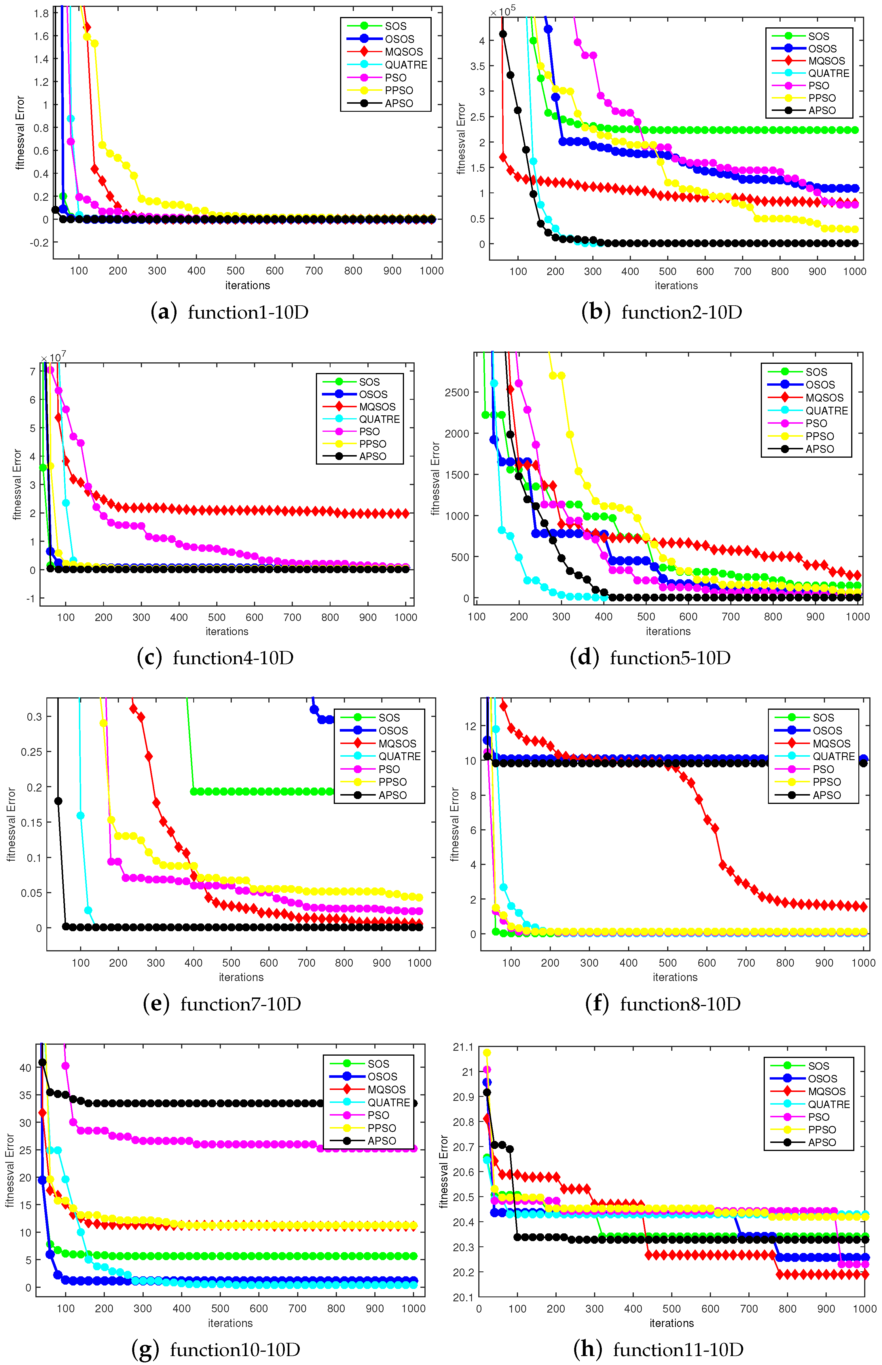
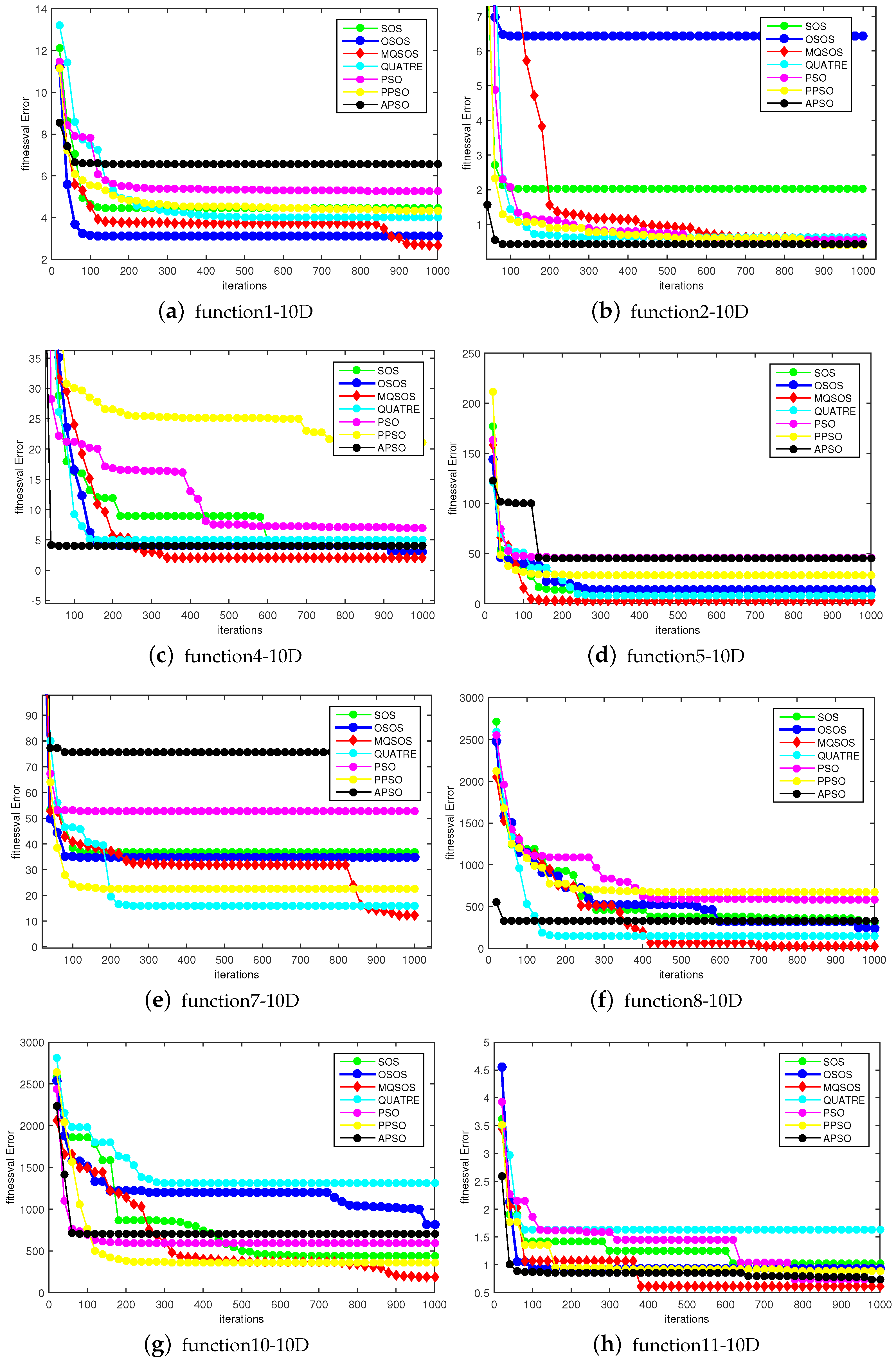
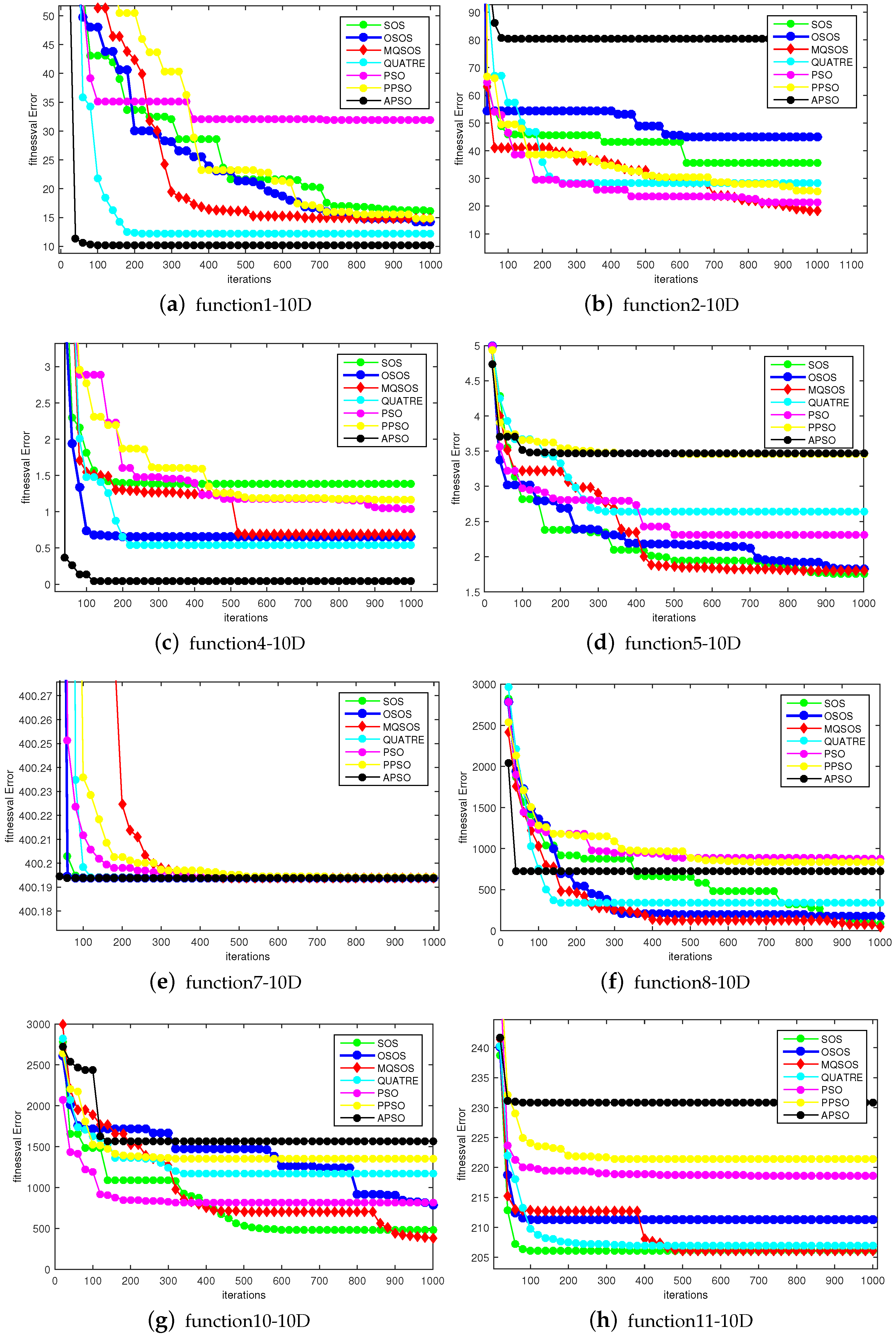
The global optimization capabilities of the seven algorithms based on the 28 benchmark functions of CEC2013 are shown in Figure 2, Figure 3, Figure 4 and Figure 5. According to the global optimization process and the final optimization result of each algorithm in these figures, the MQSOS algorithm was superior to the other algorithms in 15 benchmark functions ($f_8$, $f_9$, $f_{11}$, $f_{12}$, $f_{13}$, $f_{14}$, $f_{15}$, $f_{16}$,$f_{18}$, $f_{20}$, $f_{22}$, $f_{23}$, $f_{24}$, $f_{26}$, $f_{28}$). The APSO algorithm outperformed other algorithms in 8 benchmark functions ($f_1$, $f_2$, $f_3$, $f_5$, $f_{10}$, $f_{17}$, $f_{19}$, $f_{21}$). The QUATRE/best/1 algorithm outperformed other algorithms in 3 benchmark functions ($f_4$, $f_7$, $f_{27}$). The SOS algorithm obtained the optimal value in benchmark function $f_6$. The OSOS algorithm achieved this in benchmark function $f_{25}$.

4.2. Simulation Results of Applied MQSOS to Node Localization in WSN Based on DV-Hop

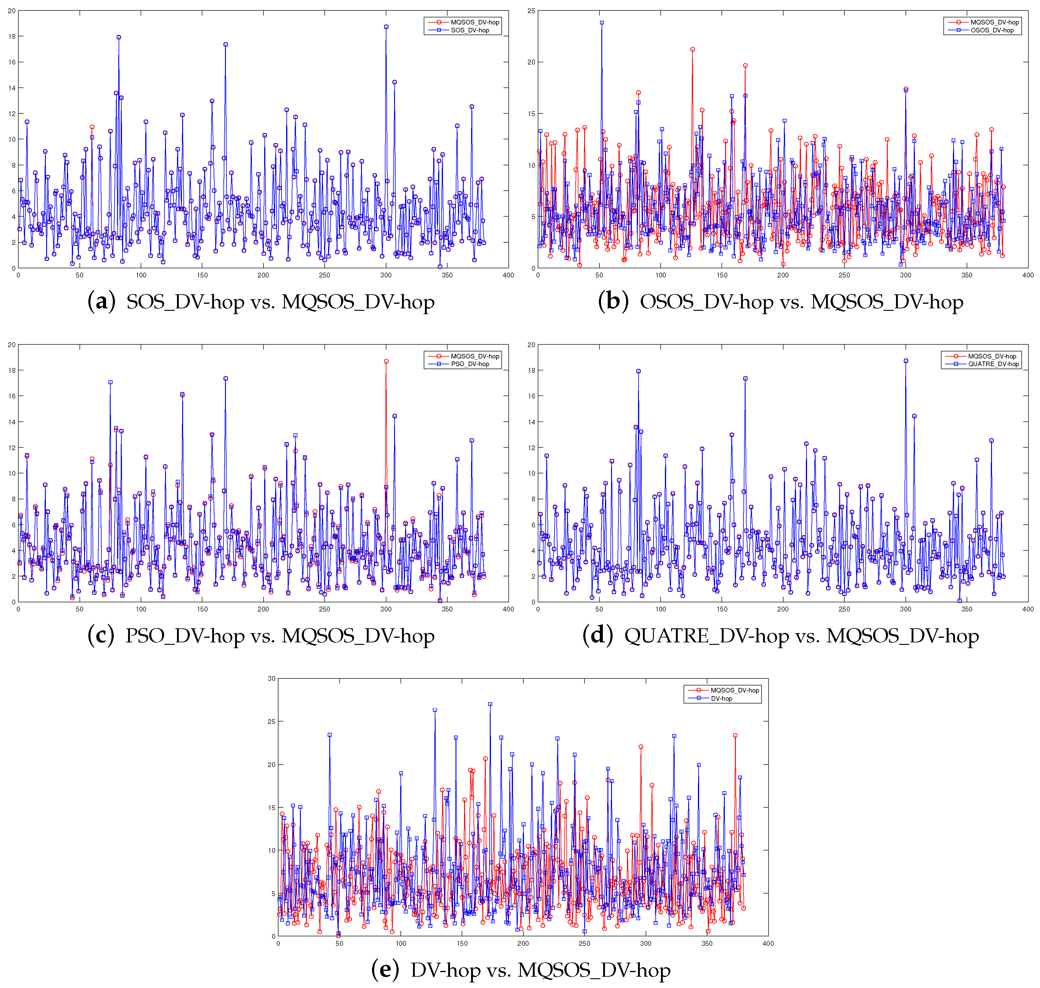
In this section, the results of the practical application of the newly proposed MQSOS algorithm in wireless node positioning are shown and compared with the results of the PSO, QUATRE/best/1, OSOS, and SOS algorithms in this application, and the performance of our proposed algorithm in practical applications is verified. In the environment simulated in this experiment, there were 20 anchor nodes and 380 unknown nodes in a two-dimensional space of 100 m × 100 m, and the communication radius of the nodes was 20 m. The results of each of these algorithms in simulation experiments are shown in

Table 3. Four positioning errors.

MQSOS_DV-hop	OSOS_DV-hop	SOS_DV-hop	QUATRE_DV-hop	PSO_DV-hop	DV-hop
$\mathbf{0.2242}$	0.2924	0.2246	0.2243	0.2924	0.4988

.

The error graphs of each unknown node of the MQSOS algorithm and other algorithms in wireless sensor positioning are shown in Figure 6. They show the sum of the errors of each node and all anchor nodes.

5. Conclusions

This paper proposes a novel SOS algorithm called the MQSOS algorithm that is based on a quantum state-based inter-group communication strategy. In the implementation process, the algorithm is first divided into several subgroups for independent iterative evolution, and the corresponding group communication is performed after each subgroup iterates to achieve the step size of inter-group communication. The quantum state-based inter-group communication strategy is used to iterate several organisms with better states in each subgroup and replace the organisms with poor states in order to enhance the convergence speed and improve the overall performance of the algorithm due to the increase of diversity. In order to verify the performance of the newly proposed MQSOS algorithm, the CEC2013 test suite was applied to compare the algorithm with other swarm intelligence algorithms. The experimental results indicate that the performance of the MQSOS algorithm was better than those of other intelligent algorithms (PSO, PPSO, original SOS, QUATRE, APSO, and OSOS algorithms). We also applied the algorithm to the location of wireless sensor nodes to form a new DV-hop algorithm called MQSOS_DV-hop, with the aim of improving the accuracy of DV-hop algorithm node positioning, and simulated the MQSOS_DV-hop wireless sensor location algorithm in Matlab. The experimental results show that the MQSOS algorithm had higher accuracy in wireless sensor network node location.

In the future, we will further study more accurate and efficient evolutionary algorithms, evolutionary programs, and communication strategies to improve the performance and efficiency of social intelligence algorithms. We also need to apply subsequent improved algorithms to different types of application scenarios, such as hierarchical routing, node deployment, clustering methods, and coverage issues in WSNs, in addition to applications in transportation, energy supply, etc.

References

- Wang, H.; Rahnamayan, S.; Sun, H.; Omran, M.G. Gaussian bare-bones differential evolution. IEEE Trans. Cybern. 2013, 43, 634–647. [Google Scholar] [CrossRef] [PubMed]
- Meng, Z.; Pan, J.S.; Tseng, K.K. PaDE: An enhanced Differential Evolution algorithm with novel control parameter adaptation schemes for numerical optimization. Knowl. Based Syst. 2019, 168, 80–99. [Google Scholar] [CrossRef]
- Zambrano-Bigiarini, M.; Clerc, M.; Rojas, R. Standard particle swarm optimisation 2011 at CEC-2013: A baseline for future pso improvements. In Proceedings of the 2013 IEEE Congress on Evolutionary Computation, Cancun, Mexico, 20–23 June 2013; pp. 2337–2344. [Google Scholar]
- Tanabe, R.; Fukunaga, A. Evaluating the performance of SHADE on CEC 2013 benchmark problems. In Proceedings of the 2013 IEEE Congress on Evolutionary Computation, Cancun, Mexico, 20–23 June 2013; pp. 1952–1959. [Google Scholar]
- Tvrdík, J.; Poláková, R. Competitive differential evolution applied to CEC 2013 problems. In Proceedings of the 2013 IEEE Congress on Evolutionary Computation, Cancun, Mexico, 20–23 June 2013; pp. 1651–1657. [Google Scholar]
- Jang, J.S.R.; Sun, C.T.; Mizutani, E. Neuro-fuzzy and soft computing-a computational approach to learning and machine intelligence [Book Review]. IEEE Trans. Autom. Control 1997, 42, 1482–1484. [Google Scholar] [CrossRef]
- Pan, J.S.; Lee, C.Y.; Sghaier, A.; Zeghid, M.; Xie, J. Novel Systolization of Subquadratic Space Complexity Multipliers Based on Toeplitz Matrix-Vector Product Approach. IEEE Trans. Very Large Scale Integr. (VLSI) Syst. 2019, 27, 1614–1622. [Google Scholar] [CrossRef]
- Pan, J.S.; Dao, T.K. A Compact Bat Algorithm for Unequal Clustering in Wireless Sensor Networks. Appl. Sci. 2019, 9, 1973. [Google Scholar]
- Wang, H.; Jin, Y.; Sun, C.; Doherty, J. Offline data-driven evolutionary optimization using selective surrogate ensembles. IEEE Trans. Evolut. Comput. 2018, 23, 203–216. [Google Scholar] [CrossRef]
- Sun, C.; Jin, Y.; Cheng, R.; Ding, J.; Zeng, J. Surrogate-assisted cooperative swarm optimization of high-dimensional expensive problems. IEEE Trans. Evolut. Comput. 2017, 21, 644–660. [Google Scholar] [CrossRef] [Green Version]
- Pan, J.S.; Hu, P.; Chu, S.C. Novel Parallel Heterogeneous Meta-Heuristic and Its Communication Strategies for the Prediction of Wind Power. Processes 2019, 7, 845. [Google Scholar] [CrossRef] [Green Version]
- Nguyen, T.T.; Pan, J.S.; Dao, T.K. An Improved Flower Pollination Algorithm for Optimizing Layouts of Nodes in Wireless Sensor Network. IEEE Access 2019, 7, 75985–75998. [Google Scholar] [CrossRef]
- Xue, X.; Chen, J.; Yao, X. Efficient User Involvement in Semiautomatic Ontology Matching. In IEEE Transactions on Emerging Topics in Computational Intelligence; IEEE: Piscataway, NJ, USA, 2018; pp. 1–11. [Google Scholar]
- Eiben, A.E.; Schoenauer, M. Evolutionary computing. Inf. Process. Lett. 2002, 82, 1–6. [Google Scholar] [CrossRef]
- Chu, S.C.; Roddick, J.F.; Pan, J.S. Ant colony system with communication strategies. Inf. Sci. 2004, 167, 63–76. [Google Scholar] [CrossRef]
- Hu, P.; Pan, J.S.; Chu, S.C.; Chai, Q.W.; Liu, T.; Li, Z.C. New Hybrid Algorithms for Prediction of Daily Load of Power Network. Appl. Sci. 2019, 9, 4514. [Google Scholar] [CrossRef] [Green Version]
- Chu, S.C.; Xue, X.; Pan, J.S.; Wu, X. Optimizing Ontology Alignment in Vector Space. J. Internet Technol. 2019. [Google Scholar] [CrossRef]
- Eberhart, R.; Kennedy, J. Particle swarm optimization. In Proceedings of the IEEE International Conference on Neural Networks, Perth, Australia, 27 November–1 December 1995; Volume 4, pp. 1942–1948. [Google Scholar]
- Tian, J.; Tan, Y.; Zeng, J.; Sun, C.; Jin, Y. Multiobjective Infill Criterion Driven Gaussian Process-Assisted Particle Swarm Optimization of High-Dimensional Expensive Problems. IEEE Trans. Evolut. Comput. 2018, 23, 459–472. [Google Scholar] [CrossRef]
- Chang, J.F.; Roddick, J.F.; Pan, J.S.; Chu, S. A parallel particle swarm optimization algorithm with communication strategies. J. Inf. Sci. Eng. 2005, 21, 809–818. [Google Scholar]
- Zhan, Z.H.; Zhang, J.; Li, Y.; Chung, H.S.H. Adaptive particle swarm optimization. IEEE Trans. Syst. Man Cybern. Part B (Cybern.) 2009, 39, 1362–1381. [Google Scholar] [CrossRef] [Green Version]
- Meng, Z.; Pan, J.S.; Xu, H. QUasi-Affine TRansformation Evolutionary (QUATRE) algorithm: A cooperative swarm based algorithm for global optimization. Knowl. Based Syst. 2016, 109, 104–121. [Google Scholar] [CrossRef]
- Liu, N.; Pan, J.S.; Wang, J.; Nguyen, T.T. An Adaptation Multi-Group Quasi-Affine Transformation Evolutionary Algorithm for Global Optimization and Its Application in Node Localization in Wireless Sensor Networks. Sensors 2019, 19, 4112. [Google Scholar] [CrossRef] [Green Version]
- Karaboga, D.; Ozturk, C. A novel clustering approach: Artificial Bee Colony (ABC) algorithm. Appl. Soft Comput. 2011, 11, 652–657. [Google Scholar] [CrossRef]
- Wang, H.; Wu, Z.; Rahnamayan, S.; Sun, H.; Liu, Y.; Pan, J.S. Multi-strategy ensemble artificial bee colony algorithm. Inf. Sci. 2014, 279, 587–603. [Google Scholar] [CrossRef]
- Tsai, P.W.; Khan, M.K.; Pan, J.S.; Liao, B.Y. Interactive artificial bee colony supported passive continuous authentication system. IEEE Syst. J. 2012, 8, 395–405. [Google Scholar] [CrossRef]
- Dorigo, M.; Gambardella, L.M. Ant colony system: A cooperative learning approach to the traveling salesman problem. IEEE Trans. Evolut. Comput. 1997, 1, 53–66. [Google Scholar] [CrossRef] [Green Version]
- Chu, S.C.; Tsai, P.W.; Pan, J.S. Cat swarm optimization. In Pacific Rim International Conference on Artificial Intelligence; Springer: Guilin, China, 2006; pp. 854–858. [Google Scholar]
- Kong, L.; Pan, J.S.; Tsai, P.W.; Vaclav, S.; Ho, J.H. A balanced power consumption algorithm based on enhanced parallel cat swarm optimization for wireless sensor network. Int. J. Distrib. Sens. Netw. 2015, 11, 729680. [Google Scholar] [CrossRef] [Green Version]
- Ezugwu, A.E.; Prayogo, D. Symbiotic organisms search algorithm: Theory, recent advances and applications. Expert Syst. Appl. 2019, 119, 184–209. [Google Scholar] [CrossRef]
- Truong, K.H.; Nallagownden, P.; Baharudin, Z.; Vo, D.N. A Quasi-Oppositional-Chaotic Symbiotic Organisms Search algorithm for global optimization problems. Appl. Soft Comput. 2019, 77, 567–583. [Google Scholar] [CrossRef]
- Zhou, Y.; Miao, F.; Luo, Q. Symbiotic organisms search algorithm for optimal evolutionary controller tuning of fractional fuzzy controllers. Appl. Soft Comput. 2019, 77, 497–508. [Google Scholar] [CrossRef]
- Ezugwu, A.E. Enhanced symbiotic organisms search algorithm for unrelated parallel machines manufacturing scheduling with setup times. Knowl. Based Syst. 2019, 172, 15–32. [Google Scholar] [CrossRef]
- Chakraborty, F.; Nandi, D.; Roy, P.K. Oppositional symbiotic organisms search optimization for multilevel thresholding of color image. Appl. Soft Comput. 2019, 82, 105577. [Google Scholar] [CrossRef]
- Liu, Z.; Sun, H.; Hu, H. Two sub-swarms quantum-behaved particle swarm optimization algorithm based on exchange strategy. In Proceedings of the 2010 Third International Symposium on Intelligent Information Technology and Security Informatics, Jinggangshan, China, 2–4 April 2010; pp. 212–215. [Google Scholar]
- Sun, J.; Xu, W.; Feng, B. A global search strategy of quantum-behaved particle swarm optimization. In Proceedings of the IEEE Conference on Cybernetics and Intelligent Systems, Singapore, 1–3 December 2004; Volume 1, pp. 111–116. [Google Scholar]
- Wang, J.; Gao, Y.; Yin, X.; Li, F.; Kim, H.J. An enhanced PEGASIS algorithm with mobile sink support for wireless sensor networks. Wirel. Commun. Mob. Comput. 2018, 2018, 1–9. [Google Scholar] [CrossRef]
- Wang, J.; Gao, Y.; Liu, W.; Sangaiah, A.K.; Kim, H.J. An intelligent data gathering schema with data fusion supported for mobile sink in wireless sensor networks. Int. J. Distrib. Sens. Netw. 2019, 15, 1550147719839581. [Google Scholar] [CrossRef] [Green Version]
- Jia, K.; Wei, Z. Water conservancy monitoring based on visual sensor networks. Int. J. Distrib. Sens. Netw. 2018, 14, 1550147718779572. [Google Scholar] [CrossRef] [Green Version]
- Zhang, F.; Ding, G.; Xu, L.; Chen, B.; Li, Z. An effective method for the abnormal monitoring of stage performance based on visual sensor network. Int. J. Distrib. Sens. Netw. 2018, 14, 1550147718769573. [Google Scholar] [CrossRef] [Green Version]
- Caballero, F.; Merino, L.; Gil, P.; Maza, I.; Ollero, A. A probabilistic framework for entire WSN localization using a mobile robot. Robot. Auto. Syst. 2008, 56, 798–806. [Google Scholar] [CrossRef]
- Chen, C.H.; Lee, C.A.; Lo, C.C. Vehicle localization and velocity estimation based on mobile phone sensing. IEEE Access 2016, 4, 803–817. [Google Scholar] [CrossRef]
- Pan, J.S.; Kong, L.; Sung, T.W.; Tsai, P.W.; Snášel, V. α-Fraction first strategy for hierarchical model in wireless sensor networks. J. Internet Technol. 2018, 19, 1717–1726. [Google Scholar]
- Li, J.; Wang, D. The Security DV-Hop Algorithm against Multiple-Wormhole-Node-Link in WSN. TIIS 2019, 13, 2223–2242. [Google Scholar]
- Li, J.; Wang, D.; Wang, Y. Security DV-hop localisation algorithm against wormhole attack in wireless sensor network. IET Wirel. Sens. Syst. 2017, 8, 68–75. [Google Scholar] [CrossRef]
- Labraoui, N.; Gueroui, M.; Aliouat, M. Secure DV-Hop localization scheme against wormhole attacks in wireless sensor networks. Trans. Emerg. Telecommun. Technol. 2012, 23, 303–316. [Google Scholar] [CrossRef]
- Barsocchi, P.; Lenzi, S.; Chessa, S.; Giunta, G. A novel approach to indoor RSSI localization by automatic calibration of the wireless propagation model. In Proceedings of the VTC Spring 2009—IEEE 69th Vehicular Technology Conference, Barcelona, Spain, 26–29 April 2009; pp. 1–5. [Google Scholar]
- Awad, A.; Frunzke, T.; Dressler, F. Adaptive distance estimation and localization in WSN using RSSI measures. In Proceedings of the 10th Euromicro Conference on Digital System Design Architectures, Methods and Tools (DSD 2007), Lubeck, Germany, 29–31 August 2007; pp. 471–478. [Google Scholar]
- Pan, J.S.; Meng, Z.; Xu, H.; Li, X. QUasi-Affine TRansformation Evolution (QUATRE) algorithm: A new simple and accurate structure for global optimization. In Proceedings of the International Conference on Industrial, Engineering and Other Applications of Applied Intelligent Systems, 29th International Conference on Industrial Engineering and Other Applications of Applied Intelligent Systems, Morioka, Japan, 2–4 August 2016; Volume 9799, pp. 657–667. [Google Scholar]
Figure 1.
Maximum likelihood estimation localization method.
Figure 2.
Comparison of the best fitnesses for functions with 10D optimization.
Figure 3.
Figure 4.
Figure 5.
Figure 6.
Comparison diagram of positioning errors between the MQSOS_DV-hop positioning algorithm and other positioning algorithms.