Article

Spatial Proximity-Based Geographically Weighted Regression Model for Landslide Susceptibility Assessment: A Case Study of Qingchuan Area, China

1
School of Civil Engineering, Central South University, Changsha 410075, China
2
Department of Civil and Environmental Engineering, Nagaoka University of Technology, Nagaoka 940-2188, Japan
*
Author to whom correspondence should be addressed.
Appl. Sci. 2020, 10(3), 1107; https://doi.org/10.3390/app10031107
Submission received: 27 December 2019 / Revised: 4 February 2020 / Accepted: 4 February 2020 / Published: 7 February 2020
(This article belongs to the Special Issue Novel Approaches in Landslide Monitoring and Data Analysis)

Abstract

:

Featured Application

Landslide susceptibility assessment and other geological disaster assessment issues.

Abstract

Landslides pose a serious threat to the safety of human life and property in mountainous regions. Susceptibility assessment for landslides is critical in landslide management strategy. Recent studies indicate that the traditional assessment models in many previous studies commonly assume a fixed relationship between influencing factors and landslide occurrence within an area, resulting in an inadequate evaluation for the local landslides susceptibility. To address this issue, in this paper we propose a spatial proximity-based geographically weighted regression (S-GWR) model considering spatial non-stationarity of landslide data for assessing the landslide susceptibility. Spatial proximity is the basic input condition for the proposed S-GWR model. The challenge lies in defining the spatial proximity expression that shows the geographical features of landslides and therefore affects the model ability of S-GWR. Our solution chooses the slope unit as spatial adjacency, rather than the grid unit in DTM. The multicollinearity between landslide influencing factors is then eliminated through variance inflation factor (VIF) method and principal component analysis (PCA). The proposed model is subsequently validated by using data in Qingchuan County, southwestern China. Spatial non-stationary is identified for landslide data. A comparison with grid unit and four traditional evaluation models is conducted. Validation results using the area under the ROC (receiver operating characteristic) curve and success rate curve indicate that the spatial proximity-based GWR model with slope unit has the highest predictive accuracy (0.859 and 0.850 respectively).

1. Introduction

Landslides are catastrophic natural hazards frequently posing risks to the major societal, economic, and environmental on an international scale [1]. According to the report from EM-DAT [2], 21,412 landslides occurred worldwide between 1900 and 2014, resulting in 38,521,499 fatalities, with 7,229,487,068 people affected and total direct economic losses exceeding $2.7 trillion.
Landslide susceptibility assessment has long been recognized as a useful tool for landslide hazard management through land use planning and better decision making in landslide prone areas [3]. It is generally based on heuristic, statistical, or deterministic models [4,5,6,7,8]. Heuristic models are subjective and much susceptible to the expectation of the results [9,10]. Deterministic models have been reported with higher accuracy, but are limited by the difficulty of obtaining detailed landslide database [11,12]. Statistical models are the most widely used models due to their simplicity and high efficiency [13,14]. Many remarkable studies on the above aspects have been made, laying a solid foundation for landslide susceptibility mapping. However, in general, most of the previous studies consider the relationship between triggering factors and landslide occurrence as a fixed effect within an area, whereas different degrees of parameter influence may occur, such that, with the change of location, the effect of parameters can be consequently changed. The uncertainties due to this varied relationship remain a scientific challenge.
The second law of geography suggests that there exists variability over space of a given relationship between variables widely in spatial data [15], which is the so-called spatial non-stationarity. In view of that landslide susceptibility assessment is heavily based on spatial data, the relationship between influencing factors and landslide susceptibility may also have the characteristics of spatial non-stationarity. Previous studies, e.g., [16], have also suggested that the effective parameters in the occurrence of a natural disaster phenomenon do not have the same importance in different parts of an area. The existence of spatial non-stationarity indicates that average relationships fitted to the whole study area of traditional models might be inappropriate since they do not accurately fit local conditions [17]. This spatial non-stationarity characteristics in the data pose difficulties in landslide susceptibility assessment based on the traditional models.
Geographically weighted regression (GWR), the most popular local regression format, shows great capability in dealing with spatial non-stationary relationships [18]. It allows the relationship between dependent and independent variables to vary over space, as well as that regression coefficients in the model are calculated for each spatial zone [19]. This method has been applied in various fields of study such as social economics, geography, and meteorology [20,21,22]. However, previous studies applying GWR model for the assessment of geological hazard susceptibility have not yet been reported.
One difficulty limiting the application of GWR model in landslide susceptibility assessment is spatial proximity. It is the basic input condition and core problem for GWR model, and the issue regarding an adequate expression for the spatial proximity at different locations directly affects the modeling ability of GWR model [23,24]. Spatial proximity is the distance relationship between two units in space, and the closer the distance, the greater the impact. The key to determining the spatial proximity is segmenting the study area into map units to effectively express the spatial adjacency relationship between landslide data. The relationship should satisfy the requirements of GWR for good internal homogeneity and between-units heterogeneity. The commonly used segmentation methods in previous studies relating to GWR model can be categorized into two major kinds, i.e., administrative units [25] and grid units [26]. Administrative unit is mostly used for social and economic issues, and its segmentation does not accord with the neighborhood characteristics of landslide data. As such, administrative unit is rarely used in geological hazard assessment. Grid unit is a popular mapping unit for susceptibility assessment since it is easily accessible, but it is not associated with geological environments. Slope unit is a relative new mapping unit for evaluating landslide susceptibility, which is generated according to hydrology theory and is the watershed area defined by drainage lines (valley lines) and water divide lines (ridge lines) [27]. It is the basic topographical unit of geological hazard occurrence. Slope unit has higher internal homogeneity and between-unit heterogeneity than grid unit. It is closely related to geological environment conditions. In this sense, slope unit provides an alternative solution for spatial proximity expression of the GWR model for landslide susceptibility assessment.
Two other key issues of GWR model are the multicollinearity elimination and the kernel function establishment. Previous studies, e.g., [28], indicated that GWR is highly susceptible to the effects of multicollinearity between explanatory variables, and collinearity among pairs of explanatory variables or multicollinearity among more than two variables often lead to problems such as parameter estimate instability and unintuitive parameter signs. These problems remain significant owing to the complicated conditions of landslide posing a high possibility of correlations between explanatory variables. Kernel function is based on the distances between observations and calibration units to place emphasis on observations that are closer in space [28]. The selection of kernel function type and the determination of its bandwidth are crucial to the spatial proximity modeling of GWR.
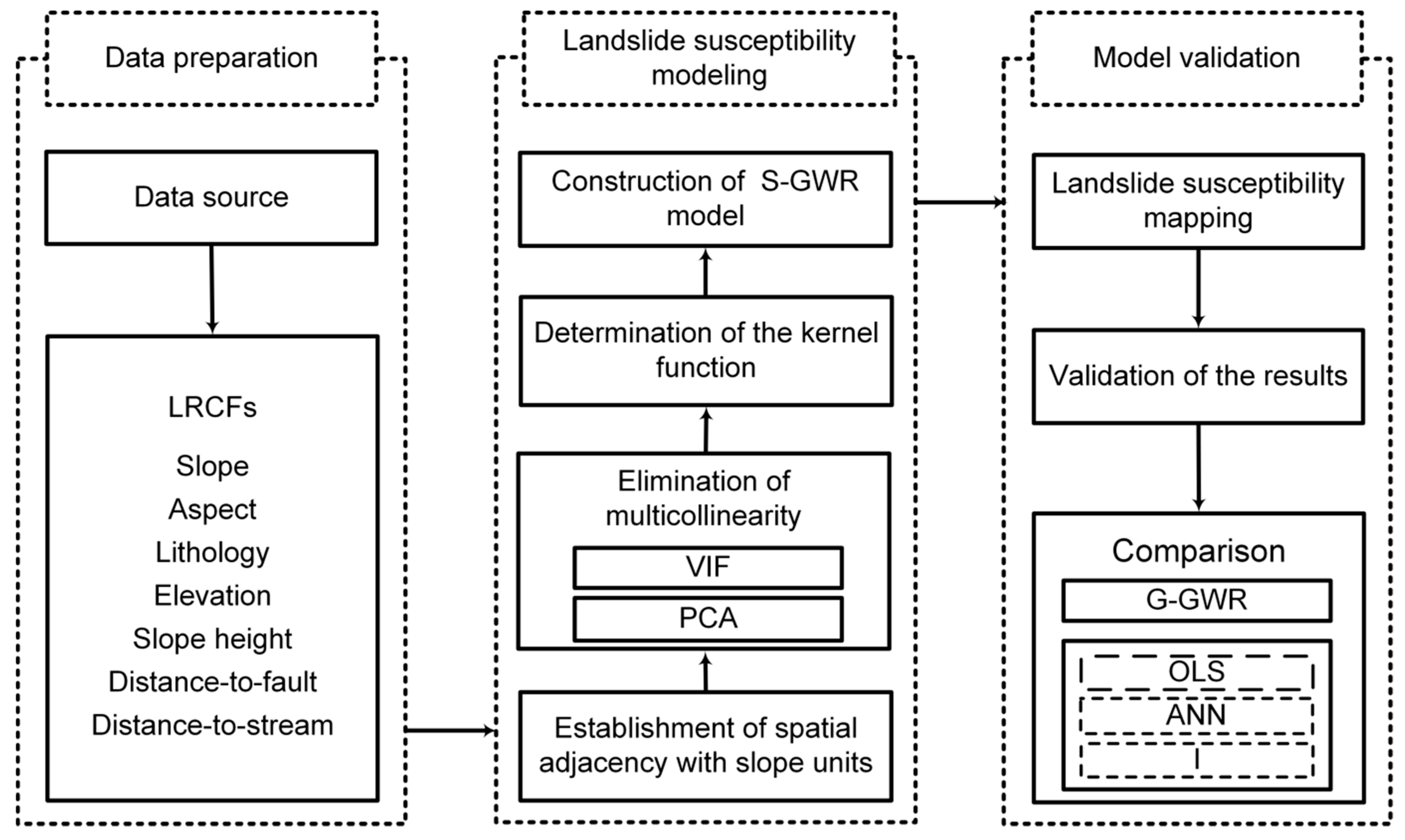
In this study, we attempt to propose a spatial proximity based on geographically weighted regression (S-GWR) model for landslide susceptibility assessment. The presented model resolves the spatial non-stationarity of landslide susceptibility assessment with GWR model. Firstly, we generate slope units to establish spatial adjacency. Then, variance inflation factor (VIF) method [29] and principal component analysis (PCA) method [30] were adopted to eliminate multi-collinearity, and kernel function was determined according to the characteristics of landslide data. Finally, we chose Qingchuan County, Sichuan Province, China, as the study area to validate the applicability of the model, and further compared the established model with the grid-unit GWR model and other evaluation models.

2. Study Area

The study area is the Qingchuan County in the transitional region between the Sichuan Basin and the Western Sichuan Plateau. This area has long been recognized as one of the most landslide-prone areas of China [31]. It locates between 32°12′~32°56′ N in latitude and 104°36′~105°38′ E in longitude, covering a total area of 3217 km2. The minimum elevation of the Qingchuan County is approximately 500 m and the maximum is 3820 m, characterized by northwestern part with higher elevation than the southeastern. Slope gradient reaches a maximum of about 80°, with a mean value of 38°.
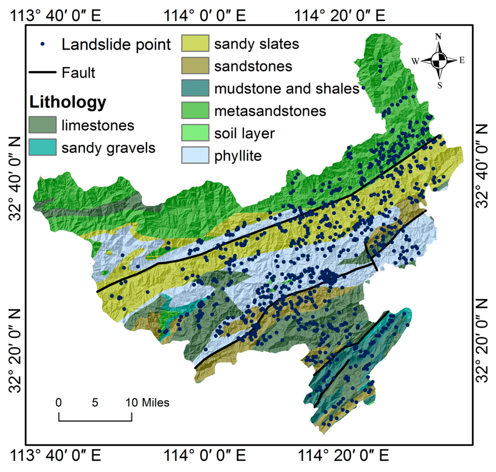
The tectonics and geological settings in the area are complex. Because of the neotectonics, soft-lithology and hard-lithology usually appears alternately. There are about eight types of lithological outcrops throughout the study region (as shown in Figure 1), including the sedimentary rock (limestones, sandstone, and conglomerate) from Cambrian to Jurassic age, magmatic (granite), metamorphic rock (shales, schists, gneiss) from Cambrian to Jurassic age and Quaternary loess unconsolidated sedimentary. Two main active faults cross the area: the Pingwu–Qingchuan fault located in the north and crossing the whole territory, and the Yingxiu–Beichuan fracture which belongs to the Longmenshan fault belt, is a thrust fault 60°–70° NW dipping. Bailong river, Qingzhu river and Qiaozhuang river are distributed in the area. The discharges of the three rivers are measured approximately 525, 30, and 40 m3s−1, respectively, serving as the main channel for atmospheric precipitation and groundwater drainage.

3. Methodology

3.1. Flowchart of Research

The methodologies used in this study are as shown in Figure 2. The flowchart consists of three major steps.
The first step is dataset preparation, including the preparation of basic data and the determination and extraction of landslide-related causal factors (LRCFs);
The second step is the establishment of the landslide susceptibility assessment model, which is the most critical step. Firstly, slope units are generated to establish spatial adjacency of landslide data. After obtaining the data in the slope units, the multicollinearity between data is eliminated by variance inflation factor method (VIF) and principal component analysis (PCA). Then, the spatial kernel function of GWR model is determined, and finally the GWR model based on slope unit (S-GWR) is established for landslide susceptibility evaluation.
The last step is model validation, including applying the S-GWR model to the actual area and generating the landslide susceptibility. The results are then used for validation and compared with the grid-unit GWR model (G-GWR) and other evaluation models including ordinary least squares regression (OLS), artificial neural network (ANN), and information models (I).

3.2. Dataset Preparation

The basic data utilized in the study include the digital elevation model (DEM) of the study area with a spatial resolution of 10 m; a geological map with the scale of 1:100,000; aerial photographs taken by Ministry of Land and Resources. After field identification and interpretation of the color aerial photographs, 973 landslide points are identified, and the distribution is as shown in Figure 1.
Owing to that a variety of factors make a contribution to the landslide occurrence, an adequate selection of the effective parameters is essential to identify areas prone to landslide. We choose these factors in accordance with the well-illustrated criterion in many previous studies (as listed in Table 1). In detail, firstly, the actual conditions of research area are considered. The study area has a complex topography, so topographic factors, such as slope and slope height, provide terrain conditions for landslides. The alternating appearance of soft and hard lithology provides a material basis for the development of landslides. Besides, there are two large faults across the study area, and the landslide frequency may increase as the distance to a major or minor fault decreased [26]. There are also many river systems in the study area. In the dense-river-areas, with the increase of catchment area and reduction of erosion basis, the shearing force of river flow is enhanced, which gives rise to the steep gorges in the downstream and provides premise conditions for the growth of geological disasters.
Based on the analysis of the research area, the factors commonly used in previous studies on landslide susceptibility are further referenced (Table 1), and 7 variables (elevation, slope, slope height, aspect, distance-to-stream, distance-to-fault, and lithology) are finally identified for modeling. All these factors are processed within ArcGIS. Slope, elevation, slope height, and aspect are calculated using DEM. All data are directly obtained by ArcGIS without data transformation. Lithology map is digitized from the existing geological map. Lithology map is digitized from the existing geological map. Distance-to-fault is obtained by calculating the distance to the nearest fault, and distance-to-stream is the distance to the nearest stream.

3.3. Establishment of Spatial Proximity

Spatial proximity is the distance relationship between two units in space. GWR model establishes a model for each unit according to the spatial proximity, and the areas within a unit are considered homogeneous. Therefore, it is essential to determine the spatial adjacency relationship between units, i.e., the boundary of map units. Administrative boundaries [25] and grid boundaries [26] were commonly used as the spatial proximity expressions of GWR in previous studies, but they are inconsistent with the neighborhood characteristics of landslides. These boundaries could not perform well to express the heterogeneity between units and the homogeneity within units, affecting the modeling ability of GWR model.
Therefore, we incorporate the methodology of slope units to express spatial proximity. Slope unit is the basic unit of geological disasters. It divides the terrain into mapping units with similar hydrological and geomorphological conditions, and is shaped by similar processes occurring in the natural landscape under the same geo-environmental conditions [37]. A slope unit division map is formed by the GIS-based hydrologic analysis tool [38]. Firstly, reverse DEM is generated by subtracting the elevation value from the highest elevation value in each unit. Secondly, fill the DEM and reverse DEM, and the flow direction can be obtained by these filled DEMs. Then, by setting the minimum number of cells that flow to the calculating point, the watershed can be calculated. Eventually, by combining the watershed by DEM and the watershed by reverse DEM, slope units can be obtained.

3.4. Elimination of Multicollinearity

Collinearity among pairs of explanatory variables or multicollinearity among more than two variables in regression analysis is known to cause problems such as parameter estimate instability, unintuitive parameter signs, high coefficient of determination (R2) diagnostics despite few or no significant parameters, and others [28]. Due to the huge and complex landslide data, the complicated relationship between geological and topographical factors should be considered. Therefore, the multicollinearity elimination in landslide susceptibility assessment is very important. Correlations in GWR parameters, both within a set of local parameter estimates for all locations (global multicollinearity) and among different parameter estimates at each location (local multicollinearity), are the symptom of multicollinearity among explanatory variables [28].
Global multicollinearity of the entire area can be easily distinguished by the variance inflation factor (VIF) method [29], which measures the effect of collinearity on the estimated variance of a regression coefficient. Local multicollinearity is the linear dependencies in the design matrix of local regression model. Principal component analysis (PCA) [30] is adopted to eliminate local multicollinearity since the diagnosis of local multicollinearity is very complicated. Through data transformation and processing, the influencing factors of landslide susceptibility can be grouped into less integrated factors, which not only maintains the main information of original factors, but also weakens the correlation among them. First obtained initial factor loading matrix. There are two main principles for selecting the principal component: (1) the principal component eigenvalue is greater than 1; (2) the cumulative contribution rate of principal components reaches 80%. Then, the factor rotation is performed so that the obtained factors have clear professional interpretation significance. Quartimax method [39], a common factor rotation method, was used for factor rotation.

3.5. GWR Modeling

GWR model extends the ordinary least squares regression (OLS) [40] by weighting the spatial dependence [41]. Based on the established spatial proximity, the coefficients of the model are estimated for each unit, and the value and symbol of the coefficients vary at different units [16]. This model is in the form of Equation (1)
y i   =   β 0 ( μ i , v i ) + j   =   1 p β i j ( μ i , v i ) x i j + ε i
where ( μ i , v i ) represents the coordinates of an ith unit in space and p is the number of independent factors. x i j is the jth independent variable of the ith unit. β 0   ( μ i , v i ) is the intercept parameter in position i and ε i is the random error. β i j   ( μ i , v i ) is the local regression coefficient for the jth explanatory variable in position i , which varies with the change of spatial position and is a very important parameter for the embodiment of spatial non-stationary.
The establishment of the weight kernel function is an important step of GWR, which is used to determine the scope and degree of spatial dependence. The establishment process includes the selection of the type of kernel function and the determination of its bandwidth, and previous studies have found that the latter has a greater impact on the result of GWR than the former [42]. This paper used a common kernel function, Gauss kernel function [43], as the type of kernel function. Its function form is
w i j   =   e x p ( ( d i j / b ) 2 )
where w i j is the weight for unit j in the neighborhood of unit i , and d i j is the distance between the center point of the unit i and j as the measurement of spatial proximity degree. b is the bandwidth of the Guass kernel function. Many approaches are available for determining the bandwidth, including cross-validation (CV) method [42], Akaike information criterion (AIC) method [44]. Compared with CV method, AIC method is easier to avoid over-fitting problems, and the selected optimal model is often more effective. Therefore, the AIC method was adopted, and the bandwidth corresponding to the weight function with the minimum AIC value is the optimal bandwidth. Equation (3) is used for the calculation of AIC,
A I C = 2 n ln ( σ ^ ) + n ln ( 2 π ) + n [ n + t r ( S ) n 2 t r ( S ) ]
where t r ( S ) is the function of b , and σ ^ is the maximum likelihood estimation for GWR model.

3.6. Validation Processes

The GEZM validation process is important; without this, the study lacks scientific credibility. In this research, we first compare the prediction results with actual units free of or containing landslides [45]. Sample points with 30% of the number of units, accounting for totally 291 landslide points, are randomly selected. The values of the predicted result belonging to the low-susceptibility and very-low-susceptibility area are regarded as the stable points and the others are as the unstable points. Then, calculate the missing rate, which is the ratio of actual unstable slopes classified as stable slopes.
Although the missing rate is one indicator that evaluates the model results, the results are subject to the threshold value, which limits the accuracy of results [46]. Therefore, we introduced ROC curve [47] and success rate curve [34] for further evaluation. The two methods are independent of the specific decision threshold and are able to further verify the accuracy of the result. ROC curve method is a measure of the ability to discriminate landslides from non-landslide locations. Success rate curve, different from the ROC curve, only considers the prediction of the landslide samples. The areas under the curve (AUC) for ROC curve and success rate curve (0.5 to 1.0) are used to assess the accuracy of the models.

4. Results

4.1. Landslide Susceptibility Map Using the Proposed Model

Based on the hydrologic analysis tool in ArcGIS environment, we segment the topography of the study area into 55,899 slope units in total. The schematic diagram of slope units is shown in Figure 3.
Firstly, in order to test the global multicollinearity, the variance inflation factor (VIF) value of each influencing factor is calculated (results shown in Table 2). A greater VIF value indicates a greater multicollinearity of the influencing factors. A value greater than 10 denotes that multicolinearity problems may exist. In this case, elevation factor for instant, the maximum VIF value is 1.88, which is apparently lower than 10. Table 2 indicates that all of the influencing factors used in the proposed S-GWR model pass the global multicollinearity test.
Then, the local multicollinearity problem is subsequently processed with PCA method. According to the principles of selecting principal components, four principal components are selected in our study, and the components explained 81.10% of the total variances. After the factor rotation, four new principal components were obtained. As is shown in Table 3, the accumulative loadings of four principal components decrease systematically. The first component can be interpreted as geological factor, as it has high positive loadings of distance-to-fault and lithology. The second component has high positive loadings of slope and slope height, indicating that this component represents slope shape factor. In the same way, the third and the fourth component represent hydrographic factor and aspect factor, respectively.
The S-GWR model is constructed using the Gaussian kernel function and the AIC method. The neighbors of the model estimated by the AIC method is 1000. According to the prediction results, landslide susceptibility of Qingchuan County is mapped. The landslide susceptibility map is classified into five classes based on the natural breaks method [48], including very low, low, moderate, high, and very-high (shown in Figure 4). The landslide susceptibility map shows that the high-susceptibility area and very-high-susceptibility area are highly consistent with the actual landslide points, and very-low- to very-high-susceptibility classes occupy 46.37%, 25.67%, 17.62%, 8.69%, and 1.65% of study area.

4.2. Validation of the S-GWR Models

4.2.1. Validation of the Spatial Non-Stationary

In order to validate the spatial non-stationary of the S-GWR model, we explore the spatial distribution of the regression coefficients between four principal components and landslide susceptibility. Results are shown in Figure 5. The coefficients estimated by S-GWR vary greatly with districts in space. This result implies a noticeable spatial non-stationarity of the relationship between four principal components and landslide susceptibility. The regression coefficients of each component have positive and negative values, which indicates that the relevance between each influencing factor and landslide susceptibility has varying direction and strength in space.
Spatial distribution of the regression coefficient of geological factors is approximately from northeast to southwest, similar to the distribution of actual lithology features and fault zones. The coefficient values of geological factors tend to decrease with the increase of the distance to fault zone and the large absolute values are mainly distributed in the metasandstones, phyllite, and sandy slates area. The distribution area with large absolute values of the coefficients of slope shape factor consist of the actual landslide points. In most of the eastern part of the study area, slope shape factor is positively correlated with landslide susceptibility, but the opposite effect exists in some central regions. The majority of the coefficient of hydrographic factor is negative, indicating that there is a significant negative correlation between the distance-to-stream and landslide susceptibility in most regions. This correlation is quite obvious in the central area, where most of the landslides occurred, such as Chaoba township, Courtyard Hui township, and the northeast area near the Bailong river. The aspect coefficient distribution map shows that the absolute value in the eastern region is larger than that in the western region. Compared with the first three principal components, the difference between the maximum and minimum values of aspect factor coefficients is the smallest.

4.2.2. Validation of the Accuracy

In order to validate the accuracy and effectiveness of the proposed S-GWR model, we compare the prediction results with actual units free of or containing landslides. Table 4 shows the prediction result of the proposed S-GWR model. Among the 291 actual landslide points, 36 points are classified as stable points with a missing rate of 12.37%. ROC curve and success rate curve are used for further evaluation. Figure 6 shows that the AUC value of ROC curve is 0.859, and the AUC value of success rate curve is 0.850.

4.3. Comparison with Other Models

4.3.1. Comparison with Grid-Unit-Based GWR (G-GWR)

In order to verify the applicability of slope units in expressing spatial proximity of the GWR, the commonly used grid unit is adopted as a comparison. For the validity of contrast and simplicity of calculation, grid size is selected as 200 × 200 m, approximately equal to the slope unit, generating 80,264 grid units.
The following procedure is the same as the process of the proposed S-GWR. The variance inflation factor (VIF) values of each influencing factor are calculated, with the maximum test result of 2.14 (as shown in Table 5). It indicates that the original G-GWR passes the global multicollinearity test. Based on the principles of selecting principal components, G-GWR also obtained four components, including geological factor, slope shape factor, hydrographic factor, and aspect factor. The establishment of kernel function of G-GWR is the same as S-GWR.
The established G-GWR model is then applied to the landslide susceptibility assessment in Qingchuan County. The sample evaluation contingency table of the G-GWR model is shown in Table 6. It shows that 61 points of the 291 actual landslide points are classified as stable points, with a missing rate of 20.96%, which is higher than that of the S-GWR model with 12.37%. The ROC curves and success rate curves of the two models are shown in Figure 7. The AUC values of ROC curve and success rate curve of G-GWR are 0.837 and 0.827 respectively, both lower than those of S-GWR. The comparative verification of the S-GWR model and the G-GWR model shows that the S-GWR model has a better performance in classification precision, thus can better identify susceptible areas to landslide occurrence. This comparison indicates that slope unit is more suitable for GWR model in the expression of spatial relationship than traditional grid unit, in particular for the purpose of landslide susceptibility assessment.

4.3.2. Comparison with OLS, ANN, and I Models

In order to further verify the applicability and accuracy of the landslide susceptibility assessment using the GWR model, we choose the ordinary least squares (OLS) model [40], artificial neural network (ANN) model [32], and information (I) model [49] as compared models, which are commonly used for the susceptibility assessment. The slope units and grid units are adopted as the sampling units of the three models respectively.
The ROC curve and success rate curve of eight models are shown in Figure 8 and Figure 9. It can be seen from the figures that for the same unit type, the AUC values of ROC curve and success rate curve of GWR models are both higher than those of ANN, I, and OLS models. It shows that the GWR model performs better, and further implies the importance of spatial non-stationarity in landslide data sets. As to the results by the same model via different unit types, the AUC values of ROC curve and success rate curve of the models with slope unit are all higher than those of the models with grid unit. It indicates that adopting slope unit as mapping unit can express the landslide characteristics better than the traditional grid unit, highlighting that slope unit is more suitable for landslide assessment.

5. Conclusions

In this paper, a spatial proximity-based geographically weighted regression (S-GWR) model is proposed for assessing the landslide susceptibility. The presented model solves the issues of the spatial non-stationarity between landslide factors and its occurrence that usually neglected in previous landslide susceptibility assessment studies. In order to express spatial proximity properly, slope units are adopted. The multicollinearity between the data is eliminated through VIF method and principal component analysis.
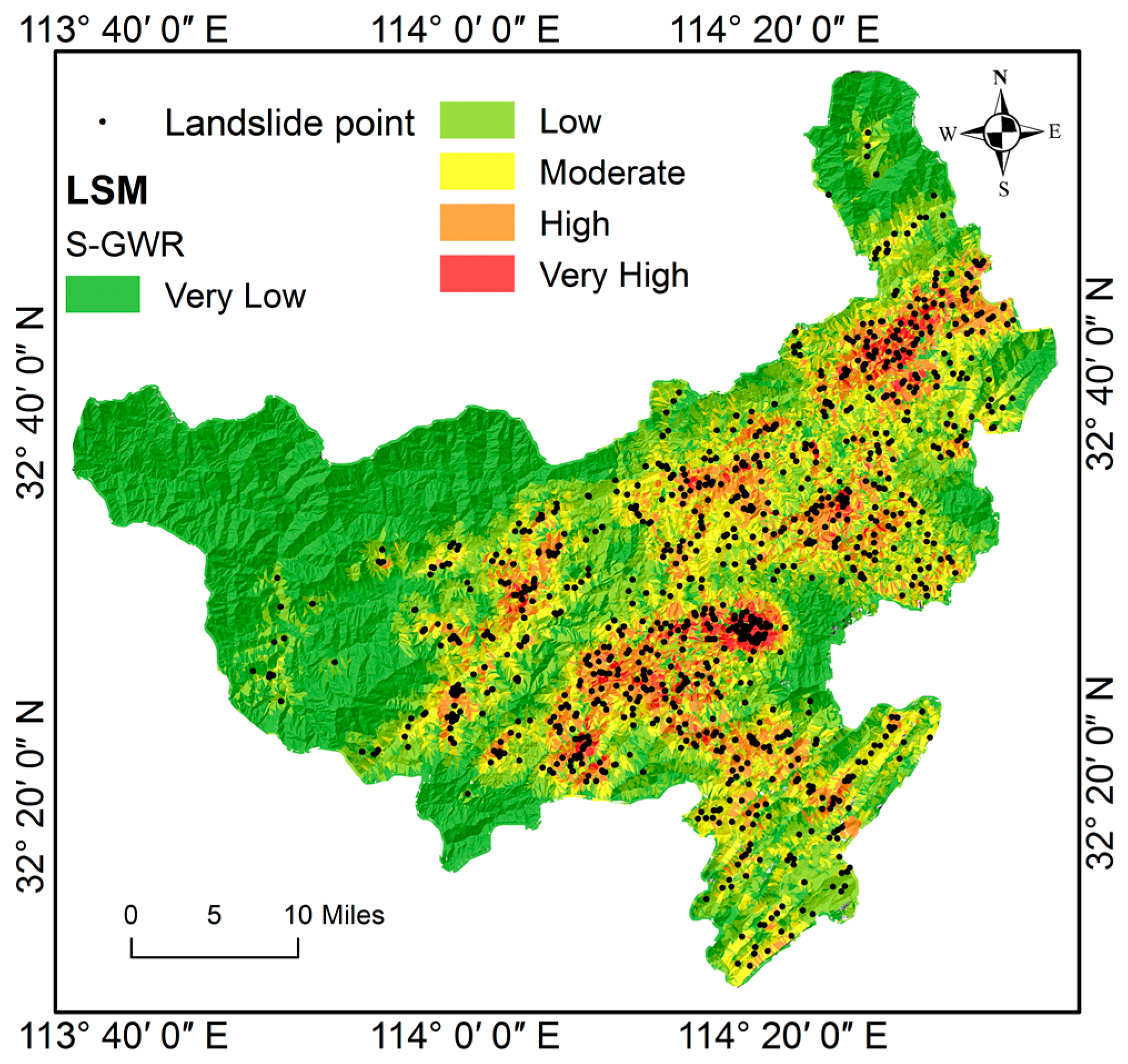
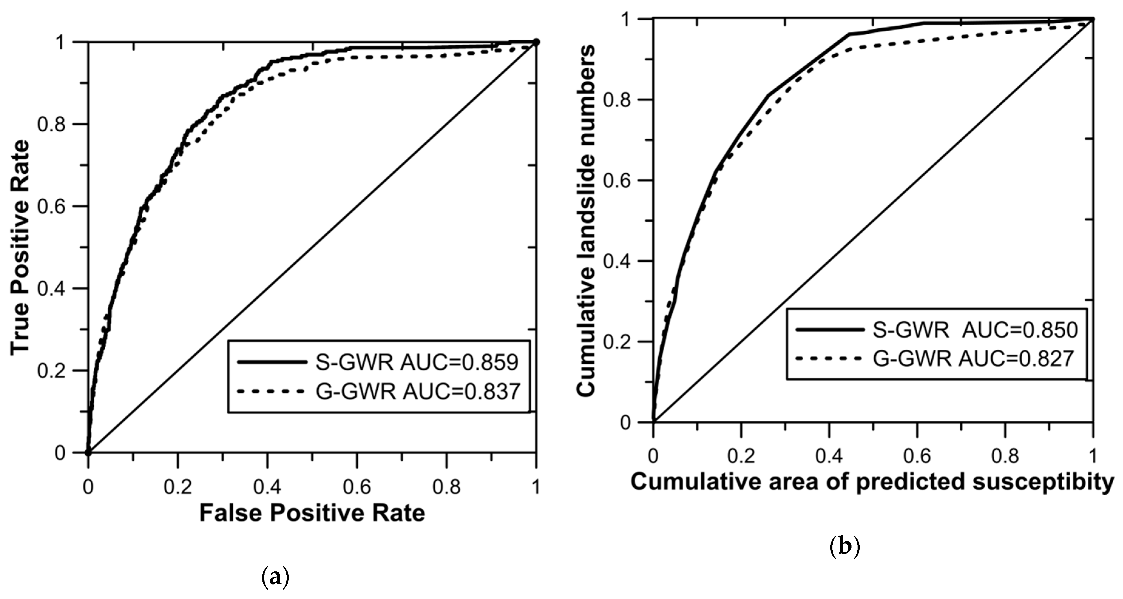
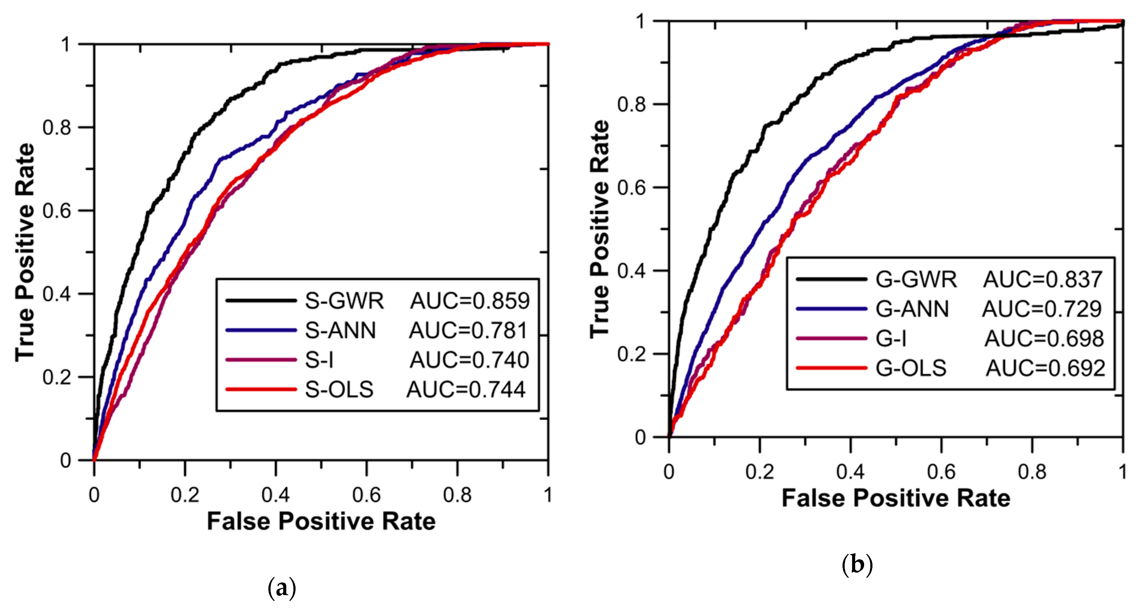
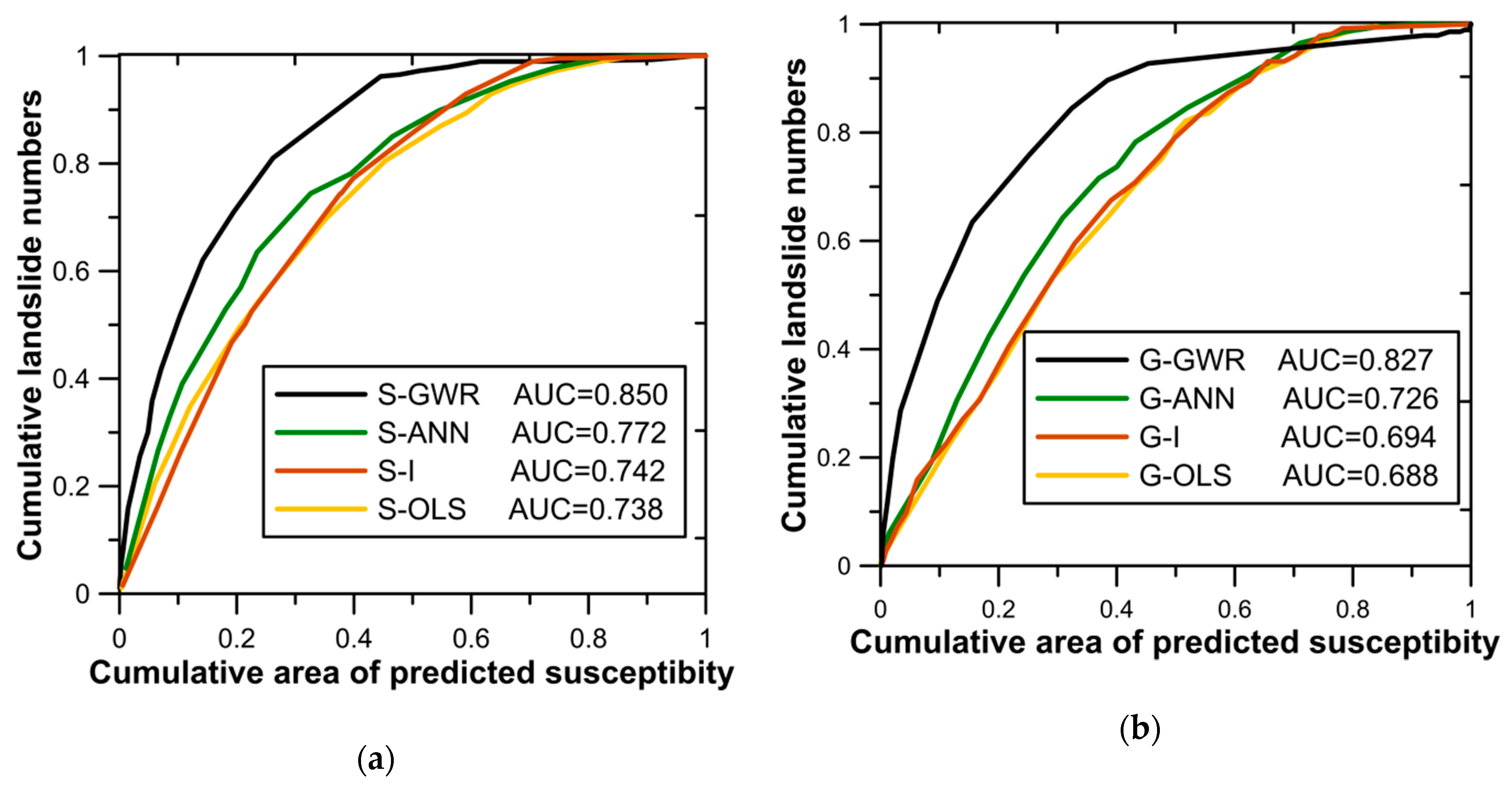
The Qingchuan area in China after the 2008 Ms. 8.0 Wenchuan earthquake is selected as a case study to illustrate the effect and validity of the proposed S-GWR model. The result shows that the four influencing factors (including geological factor, slope shape factor, hydrographic factor, and aspect factor) in the S-GWR model all have noticeable spatial non-stationary effects on the landslide susceptibility. By quantitatively testing, the missing rate of S-GWR is 12.37%, which is much lower than that of G-GWR of 20.96%, and the AUC values of ROC curve and success rate curve of S-GWR (0.859 and 0.850, respectively) are both higher than those of G-GWR (0.837 and 0.827, respectively). Besides, the AUC values of the ROC curve and success rate curve of the GWR models are higher than those of ANN, I, and OLS models, and the accuracy of each model using slope unit is higher than those of the grid unit with similar cell size.
Our study verifies the importance of considering the spatial non-stationary and the applicability of the GWR model in the landslide susceptibility assessment. It also suggests that slope unit can better express the spatial relationship between landslide data and make the evaluation results more accurate.

Author Contributions

Conceptualization and methodology, Y.L. and Z.H.; Writing—validation, X.L.; Review and editing, J.D.; All authors have read and agreed to the published version of the manuscript.

Funding

This study was financially supported by the National Key R&D Program of China (grant no. 2018YFD1100401); the National Natural Science Foundation of China (grant no. 41702310); the Natural Science Foundation of Hunan (grant no. 2018JJ3638); and the Innovation Driven Program of Central South University (grant no. 2019CX011). These financial supports are gratefully acknowledged.

Acknowledgments

We would like to thank W.W. in Central South University, China, for his constructive suggestions. We also extend our gratitude to editor-in-chief and three reviewers for their insightful comments during the review stage while we submitted the manuscript.

Conflicts of Interest

The authors declare no conflict of interest.

References

  1. Han, Z.; Su, B.; Li, Y.G.; Ma, Y.F.; Wang, W.D.; Chen, G.Q. Comprehensive analysis of landslide stability and related countermeasures: A case study of the Lanmuxi landslide in China. Sci. Rep. 2019, 9, 12407. [Google Scholar] [CrossRef] [PubMed]
  2. Guha-Sapir, D.; Below, R.; Hoyois, P. EM-DAT: International Disaster Database; Catholic University of Louvain: Brussels, Belgium, 2014; Volume 27. [Google Scholar]
  3. Pham, B.T.; Pradhan, B.; Bui, D.T.; Prakash, I.; Dholakia, M.B. A comparative study of different machine learning methods for landslide susceptibility assessment: A case study of Uttarakhand area (India). Environ. Model. Softw. 2016, 84, 240–250. [Google Scholar] [CrossRef]
  4. Pourghasemi, H.R.; Yansari, Z.T.; Panagos, P.; Pradhan, B. Analysis and evaluation of landslide susceptibility: A review on articles published during 2005–2016 (periods of 2005–2012 and 2013–2016). Arab. J. Geosci. 2018, 11, 193–205. [Google Scholar] [CrossRef]
  5. Jeong, J.S.; Ramírez-Gómez, Á. Optimizing the location of a biomass plant with a fuzzy-DEcision-MAking Trial and Evaluation Laboratory (F-DEMATEL) and multi-criteria spatial decision assessment for renewable energy management and long-term sustainability. J. Clean. Prod. 2018, 182, 509–520. [Google Scholar] [CrossRef]
  6. Mileu, N.; Queirós, M. Integrating risk assessment into spatial planning: Riskote decision support system. ISPRS Int. J. Geo Inf. 2018, 7, 184. [Google Scholar] [CrossRef] [Green Version]
  7. Abudeif, A.M.; Moneim, A.A.; Farrag, A.F. Multicriteria decision analysis based on analytic hierarchy process in GIS environment for siting nuclear power plant in Egypt. Ann. Nucl. Energy 2015, 75, 682–692. [Google Scholar] [CrossRef]
  8. Dou, J.; Yunus, A.P.; Bui, D.T.; Merghadi, A.; Sahana, M.; Zhu, Z.; Chen, C.W.; Han, Z.; Pham, B.T. Improved landslide assessment using support vector machine with bagging, boosting, and stacking ensemble machine learning framework in a mountainous watershed, Japan. Landslides 2019, 1–18. [Google Scholar] [CrossRef]
  9. Zhu, A.; Pei, T.; Qiao, J.; Chen, Y.; Zhou, C.; Cai, G. A landslide susceptibility mapping approach using expert knowledge and fuzzy logic under GIS. Prog. Geogr. 2006, 25, 1–12. (In Chinese) [Google Scholar] [CrossRef]
  10. Abella, E.A.C.; Van Westen, C.J. Qualitative landslide susceptibility assessment by multicriteria analysis: A case study from San Antonio del Sur, Guantánamo, Cuba. Geomorphology 2008, 94, 453–466. [Google Scholar] [CrossRef] [Green Version]
  11. Wu, W.; Sidle, R.C. A distributed slope stability model for steep forested basins. Water Resour. Res. 1995, 31, 2097–2110. [Google Scholar] [CrossRef]
  12. Montgomery, D.R.; Dietrich, W.E. A physically based model for the topographic control on shallow landsliding. Water Resour. Res. 1994, 30, 1153–1171. [Google Scholar] [CrossRef]
  13. Hjort, J.; Luoto, M. Statistical methods for geomorphic distribution modeling. Treatise Geomorphol. 2013, 2, 59–73. [Google Scholar] [CrossRef]
  14. Baeza, C.; Corominas, J. Assessment of shallow landslide susceptibility by means of multivariate statistical techniques. Earth Surf. Proc. Land 2001, 26, 1251–1263. [Google Scholar] [CrossRef]
  15. O’Sullivan, D. Geographically weighted regression: The analysis of spatially varying relationships. Geogr. Anal. 2003, 35, 272–275. [Google Scholar] [CrossRef]
  16. Arabameri, A.; Pradhan, B.; Rezaei, K. Gully erosion zonation mapping using integrated geographically weighted regression with certainty factor and random forest models in GIS. J. Environ. Manag. 2019, 232, 928–942. [Google Scholar] [CrossRef]
  17. Leyk, S.; Norlund, P.U.; Nuckols, J.R. Robust assessment of spatial non-stationarity in model associations related to pediatric mortality due to diarrheal disease in Brazil. Spat. Spatio Temporal Epidemiol. 2012, 3, 95–105. [Google Scholar] [CrossRef] [Green Version]
  18. Wheeler, D.C.; Páez, A. Geographically weighted regression. Int. Encycl. Hum. Geogr. 2009, 47, 407–414. [Google Scholar] [CrossRef]
  19. Düzgün, H.S.; Kemeç, S. Spatial and Geographically Weighted Regression; Springer: Boston, MA, USA, 2008. [Google Scholar] [CrossRef]
  20. Brunsdon, C.; Fotheringham, A.S.; Charlton, M.E. Geographically weighted regression: A method for exploring spatial nonstationarity. Geogr. Anal. 1996, 28, 281–298. [Google Scholar] [CrossRef]
  21. Páez, A. Exploring contextual variations in land use and transport analysis using a probit model with geographical weights. J. Transp. Geogr. 2006, 14, 167–176. [Google Scholar] [CrossRef]
  22. Tu, J. Spatially varying relationships between land use and water quality across an urbanization gradient explored by geographically weighted regression. Appl. Geogr. 2011, 31, 376–392. [Google Scholar] [CrossRef]
  23. Openshaw, S. The Modifiable Areal Unit Problem; Geo Books: Norwich, UK, 1984. [Google Scholar] [CrossRef]
  24. Wu, S. The Theory and Method of Geographically and Temporally Neural Network Weighted Regression. Ph.D. Thesis, Zhejiang University, Hangzhou, China, 2018. (In Chinese). [Google Scholar]
  25. Zhang, J.; Zhao, R. Study on the influence factors of housing price in the urban area of Bohai Ring Megalopolis based on geographically weighted regression. Territ. Nat. Resour. Study 2019, 87–93. (In Chinese) [Google Scholar] [CrossRef]
  26. Sabokbar, H.F.; Roodposhti, M.S.; Tazik, E. Landslide susceptibility mapping using geographically-weighted principal component analysis. Geomorphology 2014, 226, 15–24. [Google Scholar] [CrossRef]
  27. Ba, Q.; Chen, Y.; Deng, S.; Yang, J.; Li, H. A comparison of slope units and grid cells as mapping units for landslide susceptibility assessment. Earth Sci. Inform. 2018, 11, 373–388. [Google Scholar] [CrossRef]
  28. Fotheringham, A.S.; Oshan, T.M. Geographically weighted regression and multicollinearity: Dispelling the myth. J. Geogr. Syst. 2016, 18, 1–27. [Google Scholar] [CrossRef]
  29. Zhang, F. The Discussion on Solutions of Multicollinearity in Multilinear Regression Models. Master’s Thesis, South China University of Technology, Guangzhou, China, 2010. (In Chinese). [Google Scholar]
  30. Li, G.; Li, R.; Lu, Y.; Zhao, Y.; Yu, B. Using principal component analysis and geographic weighted regression methods to analyze AOD data. Bull. Surv. Mapp. 2018, 493, 50–56. (In Chinese) [Google Scholar] [CrossRef]
  31. Han, Z.; Li, Y.G.; Du, Y.; Wang, W.D.; Chen, G.Q. Noncontact detection of earthquake-induced landslides by an enhanced image binarization method incorporating with Monte-Carlo simulation. Geomat. Nat. Hazards Risk 2019, 10, 219–241. [Google Scholar] [CrossRef]
  32. Kawabata, D.; Bandibas, J. Landslide susceptibility mapping using geological data, a DEM from ASTER images and an Artificial Neural Network (ANN). Geomorphology 2009, 113, 97–109. [Google Scholar] [CrossRef]
  33. Li, Y.; Chen, G.; Tang, C.; Zheng, L. Rainfall and earthquake-induced landslide susceptibility assessment using GIS and Artificial Neural Network. Nat. Hazards Earth Syst. Sci. 2012, 12, 2719–2729. [Google Scholar] [CrossRef]
  34. Pradhan, B. A comparative study on the predictive ability of the decision tree, support vector machine and neuro-fuzzy models in landslide susceptibility mapping using GIS. Comput. Geosci. 2012, 51, 350–365. [Google Scholar] [CrossRef]
  35. Khan, H.; Shafique, M.; Khan, M.A.; Bacha, M.A.; Shah, S.U.; Calligaris, C. Landslide susceptibility assessment using Frequency Ratio, a case study of northern Pakistan. Egypt. J. Remote Sens. Space Sci. 2019, 22, 11–24. [Google Scholar] [CrossRef]
  36. Suh, J.; Choi, Y.; Roh, T.D.; Lee, H.J.; Park, H.D. National-scale assessment of landslide susceptibility to rank the vulnerability to failure of rock-cut slopes along expressways in Korea. Environ. Earth Sci. 2011, 63, 619–632. [Google Scholar] [CrossRef]
  37. Zhuang, J.; Peng, J.; Iqbal, J.; Liu, T.; Liu, N.; Li, Y.; Ma, P. Identification of landslide spatial distribution and susceptibility assessment in relation to topography in the Xi’ an Region, Shaanxi Province, China. Front. Earth Sci. 2015, 9, 449–462. [Google Scholar] [CrossRef]
  38. Kamp, U.; Growley, B.J.; Khattak, G.A.; Owen, L.A. GIS-based landslide susceptibility mapping for the 2005 kashmir earthquake region. Geomorphology 2008, 101, 631–642. [Google Scholar] [CrossRef]
  39. Rossoni, L.; Engelbert, R.; Bellegard, N.L. Normal science and its tools: Reviewing the effects of factor analysis in management. Rev. Adm. 2016, 51, 198–211. [Google Scholar] [CrossRef] [Green Version]
  40. Zheng, W.; Xu, W.; Tong, F.; Shi, A. 3D geological visualization and numerical modeling of complicated slope. Chin. J. Rock Mech. Eng. 2007, 26, 1633–1644. (In Chinese) [Google Scholar]
  41. Su, S.; Gong, Y.; Tan, B.; Pi, J.; Weng, M.; Cai, Z. Area social deprivation and public health: Analyzing the spatial non-stationary associations using geographically weighed regression. Soc. Indic. Res. 2016, 133, 819–832. [Google Scholar] [CrossRef]
  42. Yan, G.; Liang, S.; Zhao, H. Improvement and implementation of slope element partitioning method based on GIS. Sci. Geogr. Sin. 2017, 37, 1764–1770. (In Chinese) [Google Scholar] [CrossRef]
  43. Qin, W. The Basic Theoretics and Application Research on Geographically Weighted Regression. Ph.D. Thesis, Tongji University, Shanghai, China, 2007. [Google Scholar]
  44. Zhang, L.; Yang, Y.; Liang, X. The diagnostic approach of multicollinearity in geographically weighted regression model. Geomat. Spat. Inf. Technol. 2017, 40, 28–31. (In Chinese) [Google Scholar]
  45. Guzzetti, F.; Reichenbach, P.; Ardizzone, F.; Cardinali, M.; Galli, M. Estimating the quality of landslide susceptibility models. Geomorphology 2006, 81, 166–184. [Google Scholar] [CrossRef]
  46. Qiu, H. Study on the Regional Landslide Characteristic Analysis and Hazard Assessment: A Case Study of Ningqiang County. Ph.D. Thesis, Northwest University, Xian, China, 2012. [Google Scholar]
  47. Goetz, J.N.; Guthrie, R.H.; Brenning, A. Integrating physical and empirical landslide susceptibility models using generalized additive models. Geomorphology 2011, 129, 376–386. [Google Scholar] [CrossRef]
  48. Jenks, G. Optimal Data Classification for Choropleth Maps. Ph.D. Thesis, University of Kansas, Kansas, KS, USA, 1977. [Google Scholar]
  49. Akbar, T.A.; Ha, S.R. Landslide hazard zoning along Himalayan Kaghan Valley of Pakistan-by integration of GPS, GIS, and remote sensing technology. Landslides 2011, 8, 527–540. [Google Scholar] [CrossRef]
Figure 1. Lithological map of Qingchuan area and locations of landslide points.
Applsci 10 01107 g001
Figure 2. Methodology of research applied in this study.
Applsci 10 01107 g002
Figure 3. Schematic diagram of spatial proximity expression in slope units.
Applsci 10 01107 g003
Figure 4. Landslide susceptibility mapping (LSM) by the proposed S-GWR model.
Applsci 10 01107 g004
Figure 5. Spatial distribution of the principal component coefficient function estimate. (a) Regression coefficient of geological factor (PC1); (b) Regression coefficient of slope shape factor (PC2); (c) Regression coefficient of hydrographic factor (PC3); (d) Regression coefficient of aspect factor (PC4)).
Applsci 10 01107 g005
Figure 6. Validation of S-GWR model. (a) ROC curve; (b) success rate curve.
Applsci 10 01107 g006
Figure 7. Validation of S-GWR and G-GWR models. (a) ROC curve; (b) success rate curve.
Applsci 10 01107 g007
Figure 8. ROC curves and area under the curves (AUC) for the susceptibility maps produced by GWR, ANN, I, OLS. (a) Slope unit; (b) grid unit.
Applsci 10 01107 g008
Figure 9. Success rate curves and area under the curves (AUC) for the susceptibility maps produced by GWR, ANN, I, OLS. (a) Slope unit; (b) grid unit.
Applsci 10 01107 g009
Table 1. Criteria for a rational selection of landslide factors on the basis of literature review.
CriteriaFormer Studies Using the Same Criterion for Landslide Susceptibility Assessment
ElevationKawabata et al. (2009) [32], Li et al. (2012) [33], Sabokbar et al. (2014) [26], Pradhan. (2013) [34], HawasKhan et al. (2019) [35]
SlopeKawabata et al. (2009) [32], Li et al. (2012) [33], Sabokbar et al. (2014) [26], Pradhan. (2013) [34], HawasKhan et al. (2019) [35], Suh et al. (2019) [36], Zhuang et al. (2012) [37]
Slope heightLi et al. (2012) [33], Suh et al. (2019) [36], Zhuang et al. (2012) [37]
AspectKawabata et al. (2009) [32], Li et al. (2012) [33], Sabokbar et al. (2014) [26], HawasKhan et al. (2019) [35], Zhuang et al. (2012) [37]
Distance-to-streamLi et al. (2012) [33], Sabokbar et al. (2014) [26], Pradhan. (2013) [34], HawasKhan et al. (2019) [35]
Distance-to-faultLi et al. (2012) [33], Sabokbar et al. (2014) [26], HawasKhan et al. (2019) [35], Suh et al. (2019) [36]
LithologyKawabata et al. (2009) [32], Li et al. (2012) [33], Sabokbar et al. (2014) [26], Pradhan. (2013) [34], HawasKhan et al. (2019) [35], Suh et al. (2019) [36]
Table 2. Test results of variance inflation factor method of S-GWR.
Influencing FactorsVIF
Slope1.61
Aspect1.06
Elevation1.88
Slope height1.52
Lithology1.35
Distance-to-fault1.87
Distance-to-stream1.12
Table 3. Rotated component loadings of the indicators on selected principal components.
Principal ComponentsPC1PC2PC3PC4
Slope0.1280.8580.0470.133
Aspect0.0380.1320.0550.981
Elevation0.6750.3740.374−0.007
Slope height0.1060.861−0.152−0.010
Lithology0.829−0.030−0.1950.108
Distance-to-fault0.8600.1220.110−0.066
Distance-to-stream0.070−0.1060.9390.055
Accumulative loadings2.7062.2111.1781.194
Table 4. Sample evaluation contingency table of the proposed S-GWR model.
Predicted Groups (Model)
StableUnstable
Actual Groups (inventory)Stable11,881 (72.43%)4523 (27.57%)
Unstable36 (12.37%)255 (87.63%)
Table 5. Test results of variance inflation factor method of G-GWR.
Influencing FactorsVIF
Slope1.02
Aspect1.83
Elevation2.05
Slope height2.00
Lithology2.14
Distance-to-fault1.10
Distance-to-stream1.36
Table 6. Sample evaluation contingency table of G-GWR model.
Predicted Groups (Model)
StableUnstable
Actual groups (inventory)Stable13,449 (78.20%)3750 (21.80%)
Unstable61 (20.96%)230 (79.04%)

