Strain Influence Factor Charts for Settlement Evaluation of Spread Foundations based on the Stress–Strain Method


Department of Civil Engineering and Geomatics, Cyprus University of Technology, 2-8 Saripolou str, 3603 Limassol, Cyprus
Appl. Sci. 2020, 10(11), 3822; https://doi.org/10.3390/app10113822
Submission received: 10 May 2020
/
Revised: 19 May 2020
/
Accepted: 21 May 2020
/
Published: 31 May 2020
(This article belongs to the Section Civil Engineering)
Abstract
:Featured Application
This study is a practical tool for Civil Engineers for the settlement evaluation of spread foundations using the stress-strain method.
Abstract
In this paper, the stress–strain method for the elastic settlement analysis of shallow foundations is revisited, offering a great number of strain influence factor charts covering the most common cases met in civil engineering practice. The calculation of settlement based on strain influence factors has the advantage of considering soil elastic moduli values rapidly varying with depth, such as those often obtained in practice using continuous probing tests, e.g., the Cone Penetration Test (CPT) and Standard Penetration Test (SPT). It also offers the advantage of the convenient calculation of the correction factor for future water table rise into the influence depth of footing. As is known, when the water table rises into the influence zone of footing, it reduces the soil stiffness and thus additional settlement is induced. The proposed strain influence factors refer to flexible circular footings (at distances 0, R/3, 2R/3 and R from the center; R is the radius of footing), rigid circular footings, flexible rectangular footings (at the center and corner), triangular embankment loading of width B and length L (L/B = 1, 2, 3, 4, 5 and 10) and trapezoidal embankment loading of infinite length and various widths. The strain influence factor values are given for Poisson’s ratio value of soil, ranging from 0 to 0.5 with 0.1 interval. The compatibility of the so-called “characteristic point” of flexible footings with the stress–strain method is also investigated; the settlement under this point is considered to be the same as the uniform settlement of the respective rigid footing. The analysis showed that, despite the effectiveness of the “characteristic point” concept in homogenous soils, the method in question is not suitable for non-homogenous soils, as it largely overestimates settlement at shallow depths (for z/B < 0.35) and underestimates it at greater depths (for z/B > 0.35; z is the depth below the footing and B is the footing width).
1. Introduction
Schmertmann et al.’s [1] strain influence factor method (or stress–strain method) for immediate settlement analysis is among the most popular ones worldwide. In brief, the method in question incorporates the use of a bilinear strain influence factor Iz versus z/B relationship (z is the depth measured from the foundation level and B is the width of foundation); the area under this relationship multiplied by the net footing loading and divided by the elastic modulus of soil, E, gives the footing settlement. As Iz is depth-specific and so is the elastic modulus of soil, the method in question can take into account the fluctuation of E with depth. Schmertmann’s method has been modified by various researchers [2,3,4,5,6,7], who, however, kept the crude bilinear approximation. This semi-empirical approach is suggested by or included in various countries’ design codes and public agencies’ reference manuals, such as AASHTO, EN 1997-2 and Samtani and Nowatzki [8,9,10]. However, in the forthcoming revision of Eurocode 7 (prEN1997-3:202x), Schmertmann’s stress–strain method has been abandoned; it recommends instead the stress–strain method deriving from pure elasticity. An in-depth review of Schmertmann’s method has recently been offered by the author [11]. Indicatively, it is mentioned that independent studies [2,12,13,14,15,16,17,18,19] comparing the measured settlement of structures or full-size test footings with the respective settlement calculated with Schmertmann’s method indicate great deviation. This deviation can be attributed to the replacement of the actual curved Iz–z/B relationship with a simplistic bilinear one, the way the embedment depth is taken into account, the plastic response of the ground and the fact that Schmertmann’s method was developed considering Poisson’s ratio values in the order of 0.4 to 0.5. For the latter, Mayne and Poulos [20] pointed out that accurate measurements using local strain devices mounted midlevel on soil specimens and measured internally to the triaxial cell have shown that the appropriate value of Poisson’s ratio for use in elastic continuum solutions for drained loading is 0.1 < ν < 0.2 for all soil types [20,21,22].
Strain influence factor values derived from the theory of elasticity can be found in various sources [23,24]; however, these are example curves referring to a very limited number of cases. In the present paper, the problem in question is studied on a systematic basis, giving strain influence factors for the most common cases met in practice—i.e., for uniformly loaded flexible and rigid circular footings, uniformly loaded flexible rectangular footings and triangular and trapezoidal embankment loading. The settlement under the so-called “characteristic point” of flexible footings is also investigated; the settlement under this point is considered to be the same as the uniform settlement of the respective rigid footing. The calculation of settlement based on strain influence factors (strain–strain method) offers the advantage of considering non-uniform elastic moduli profiles with depth (e.g., linearly varying modulus with depth or different elastic moduli due to soil stratification), such as those often obtained in practice using continues probing tests—e.g., the Cone Penetration Test (CPT) and Standard Penetration Test (SPT).
2. Derivation of the Strain Influence Factor Charts
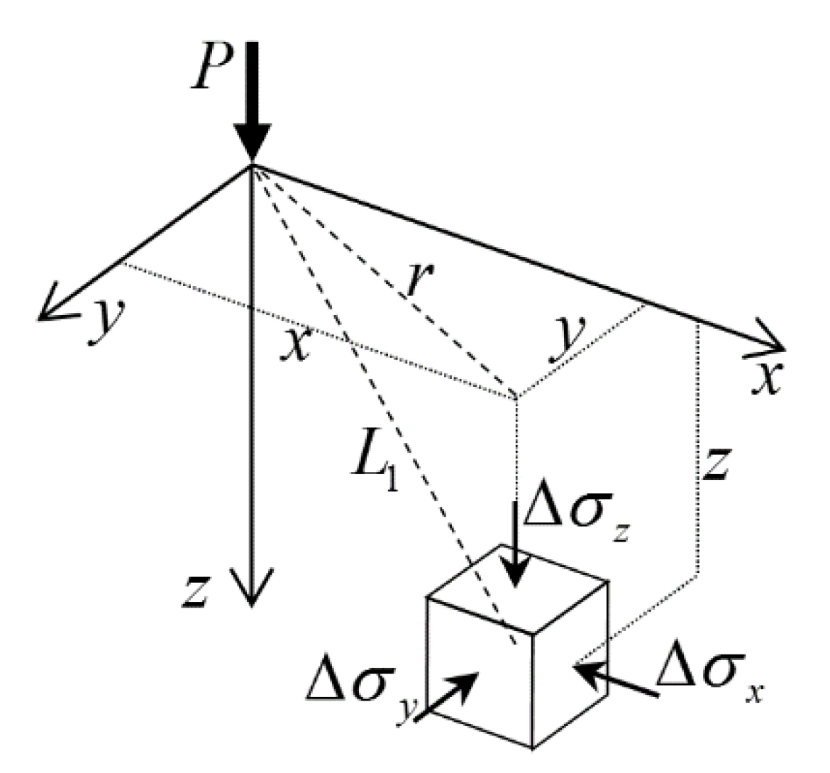
Boussinesq [25] solved the problem of stresses produced at any point in a homogenous, elastic and isotropic medium as the result of a point load applied on the surface of an infinitely large semi-space. Following the notation of Figure 1, the increase in normal stresses caused by the point load P is:
where, , and ν is the Poisson’s ratio [26].
The increase in the normal stress parallel to the i-axis due to loading over a whole surface area can be found by integrating the respective stress increase due to point loading over this area:
Note that the differentials of the variables x and y (i.e., dx and dy) are included in Δσi as the point force at an arbitrary point (x,y) on the surface of the semi-infinite mass domain is P=qdydx (recall Equations (1)–(3); q is the distributed load over the dx dy). The unit vertical strain can then be calculated from the constitutive relationship of Hooke’s law:
(E is the modulus of elasticity of the compressible medium). The latter can be rewritten as:
where, Iz is the non-dimensional strain influence factor:
The settlement, ρ, at depth zα corresponding to a layer extending from zα to a lower depth zb derives from the integration of Equation (6) between these depths (apparently, at the foundation level, zα equals zero):
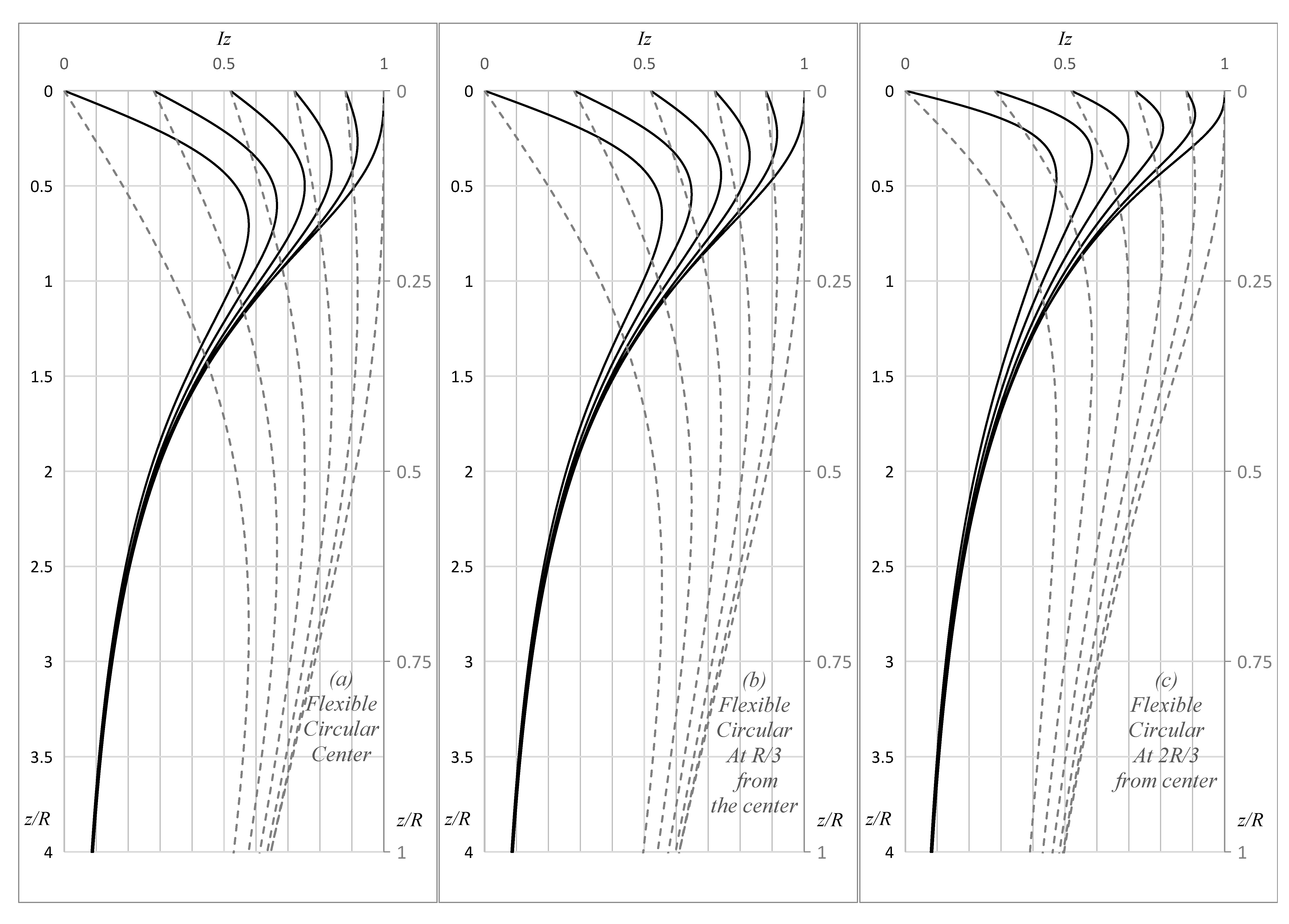
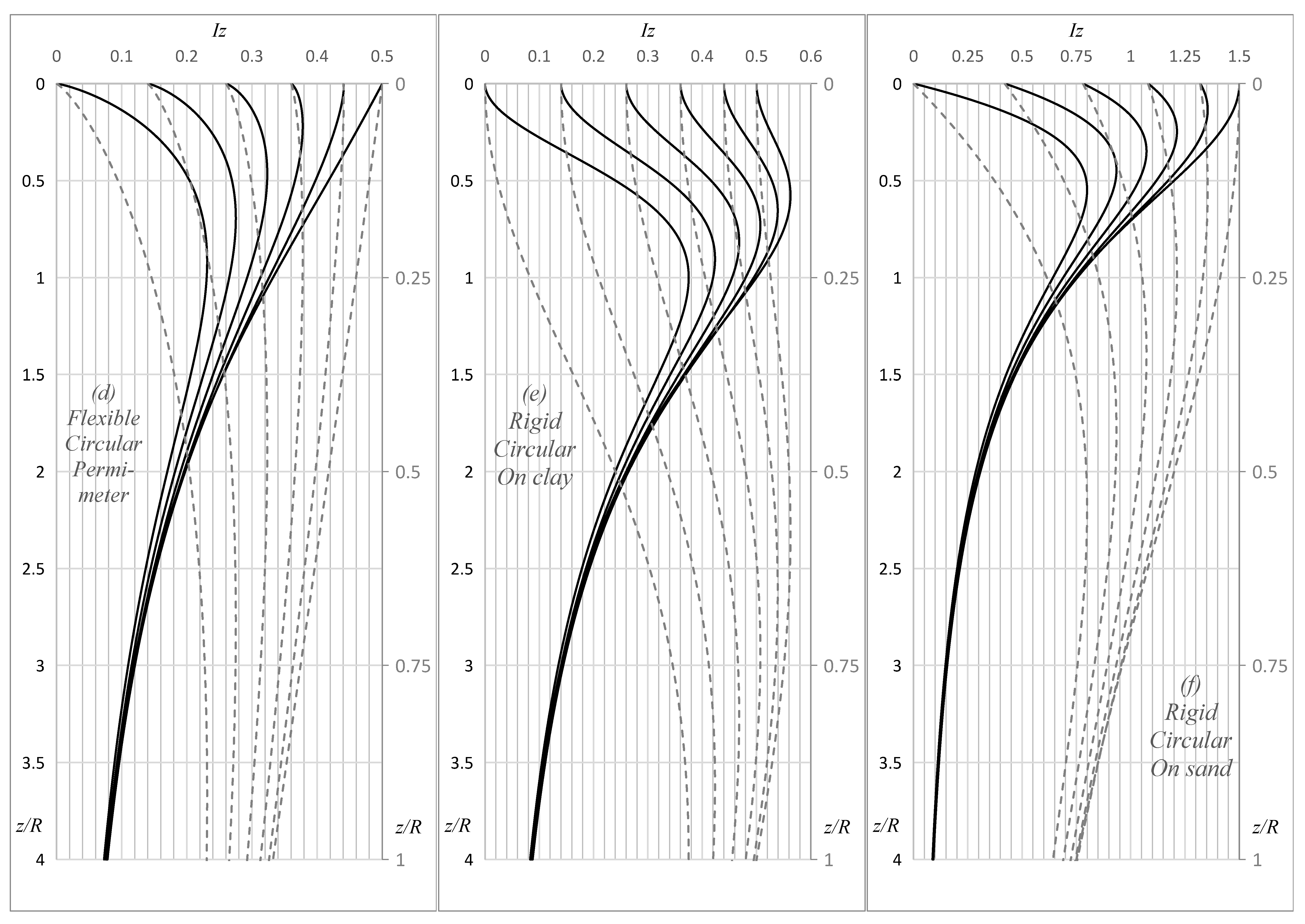
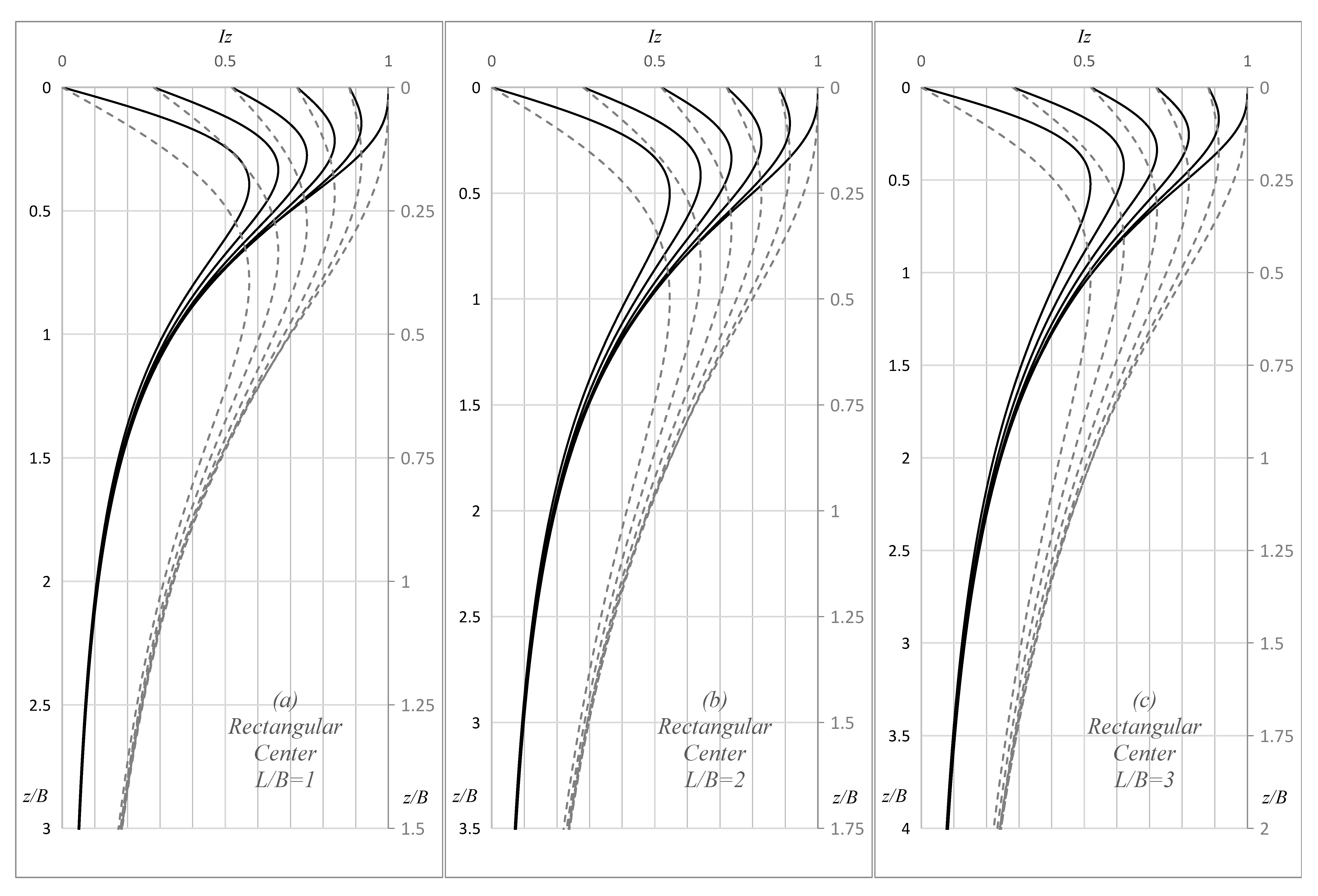
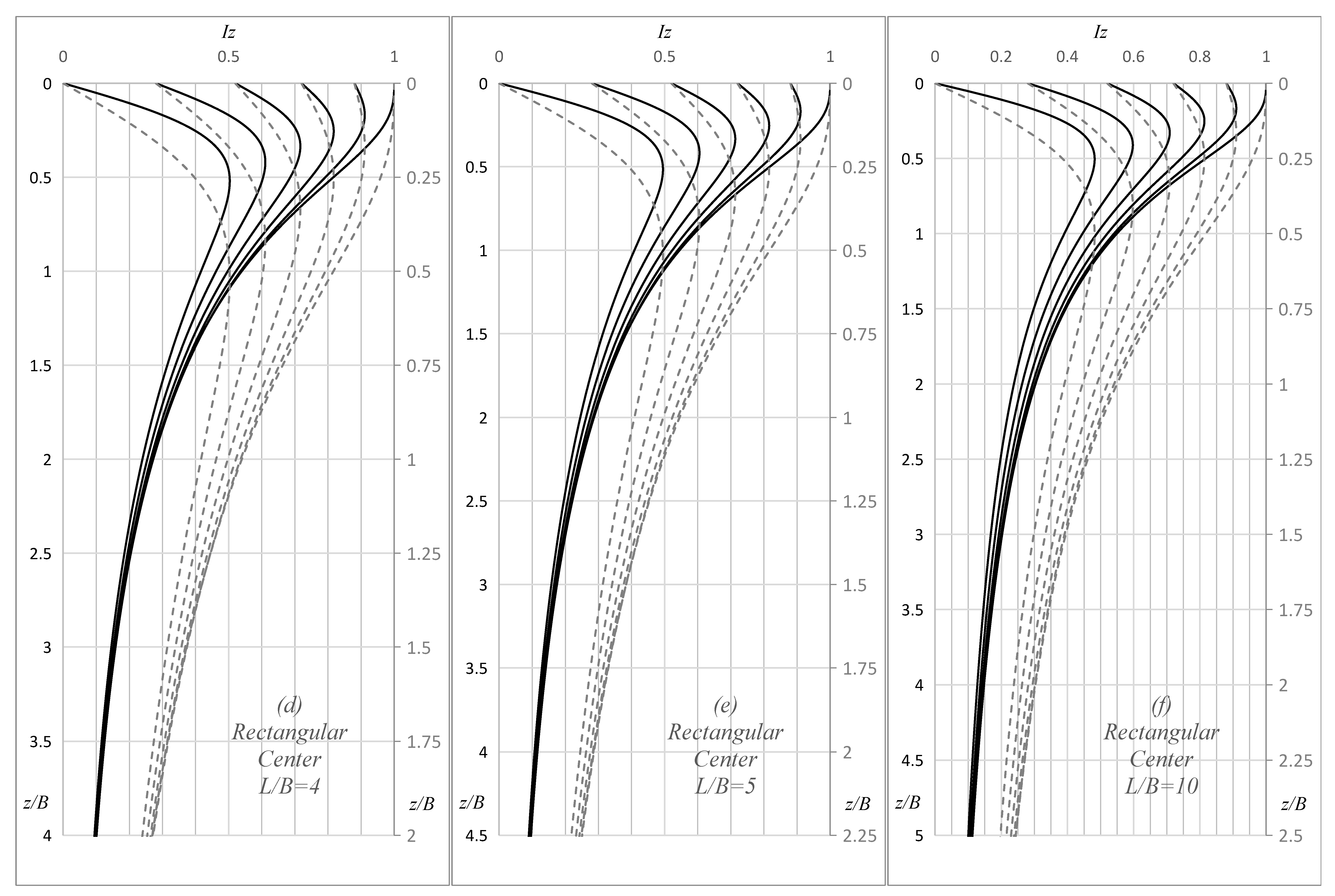
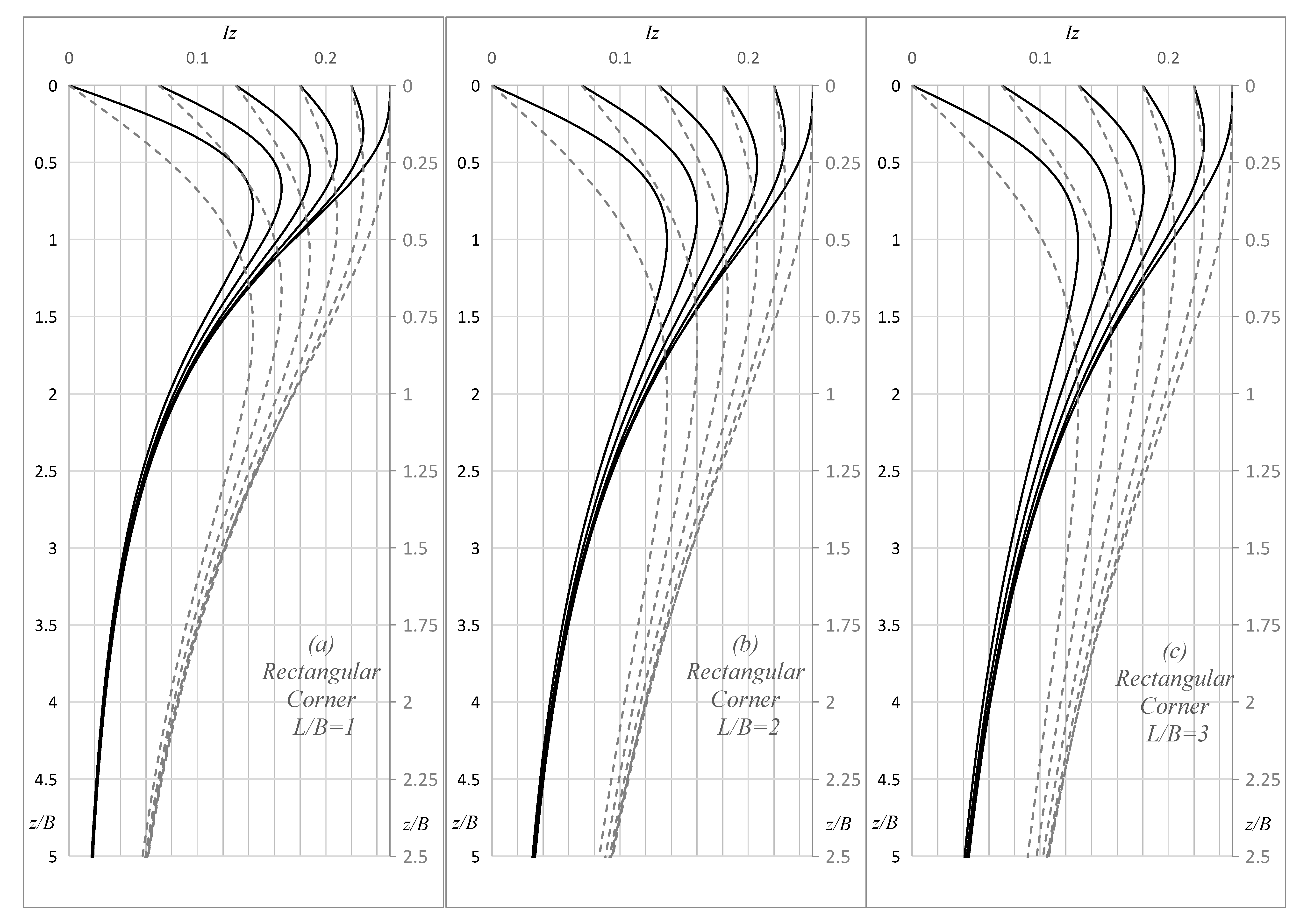
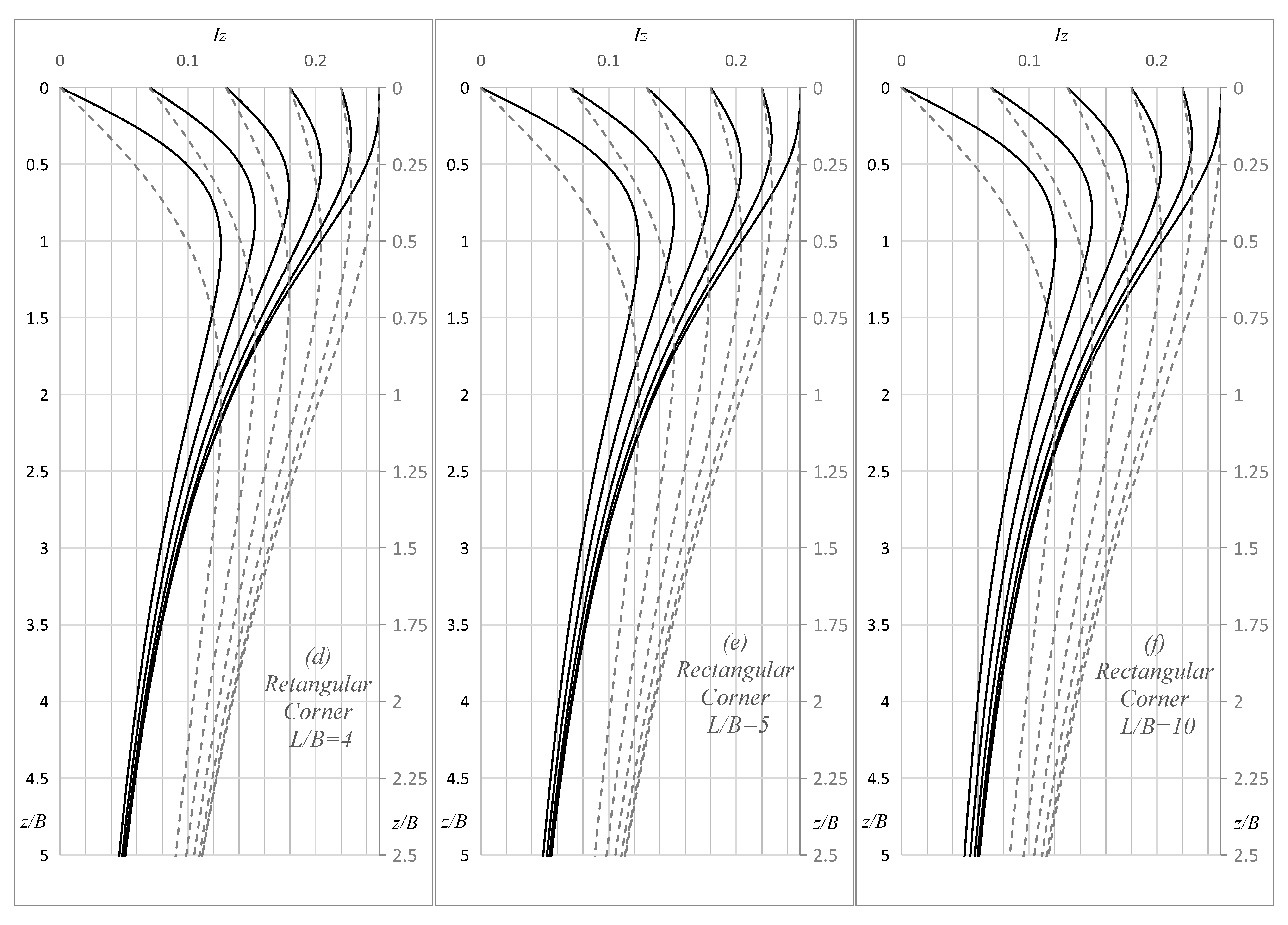
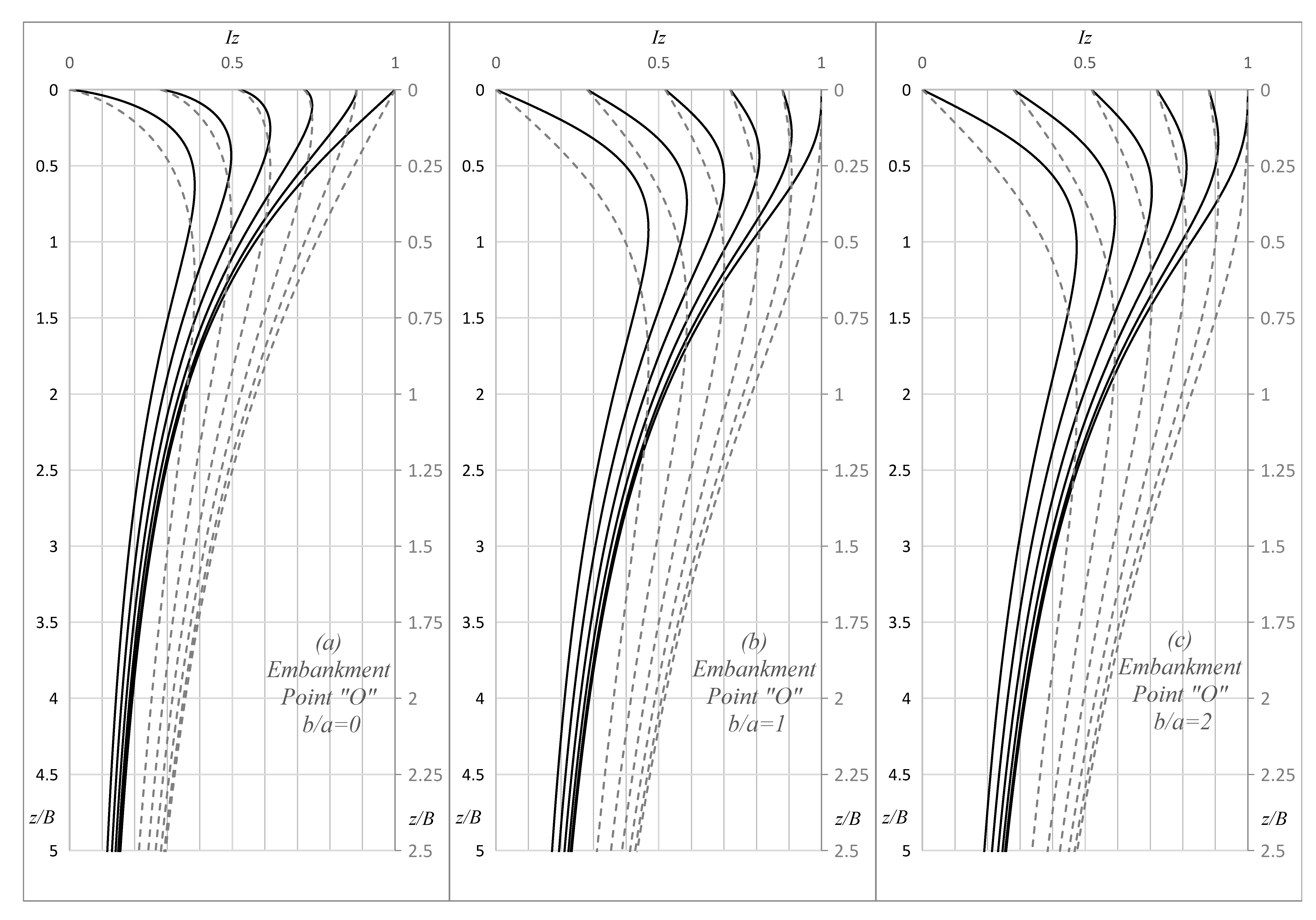
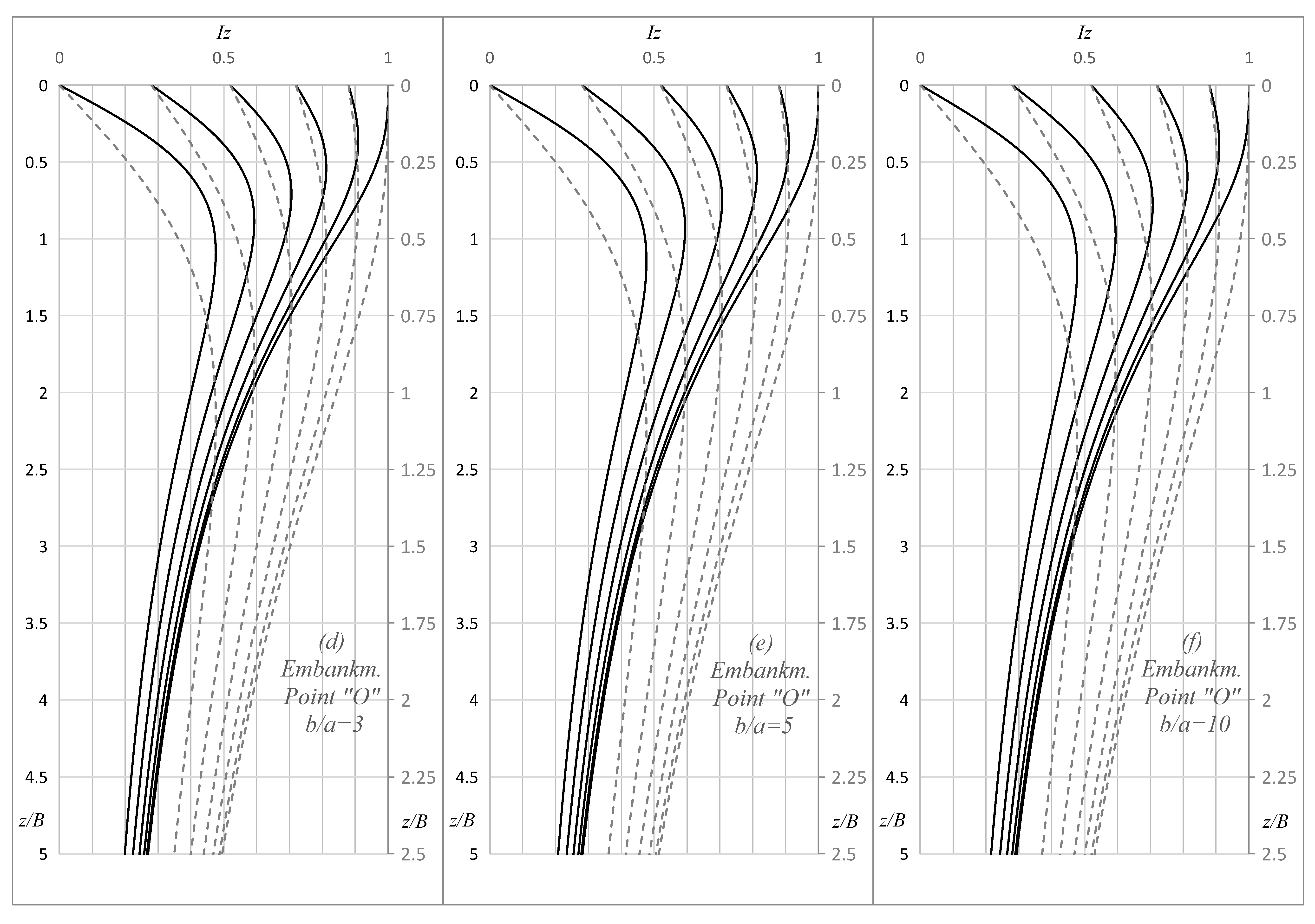
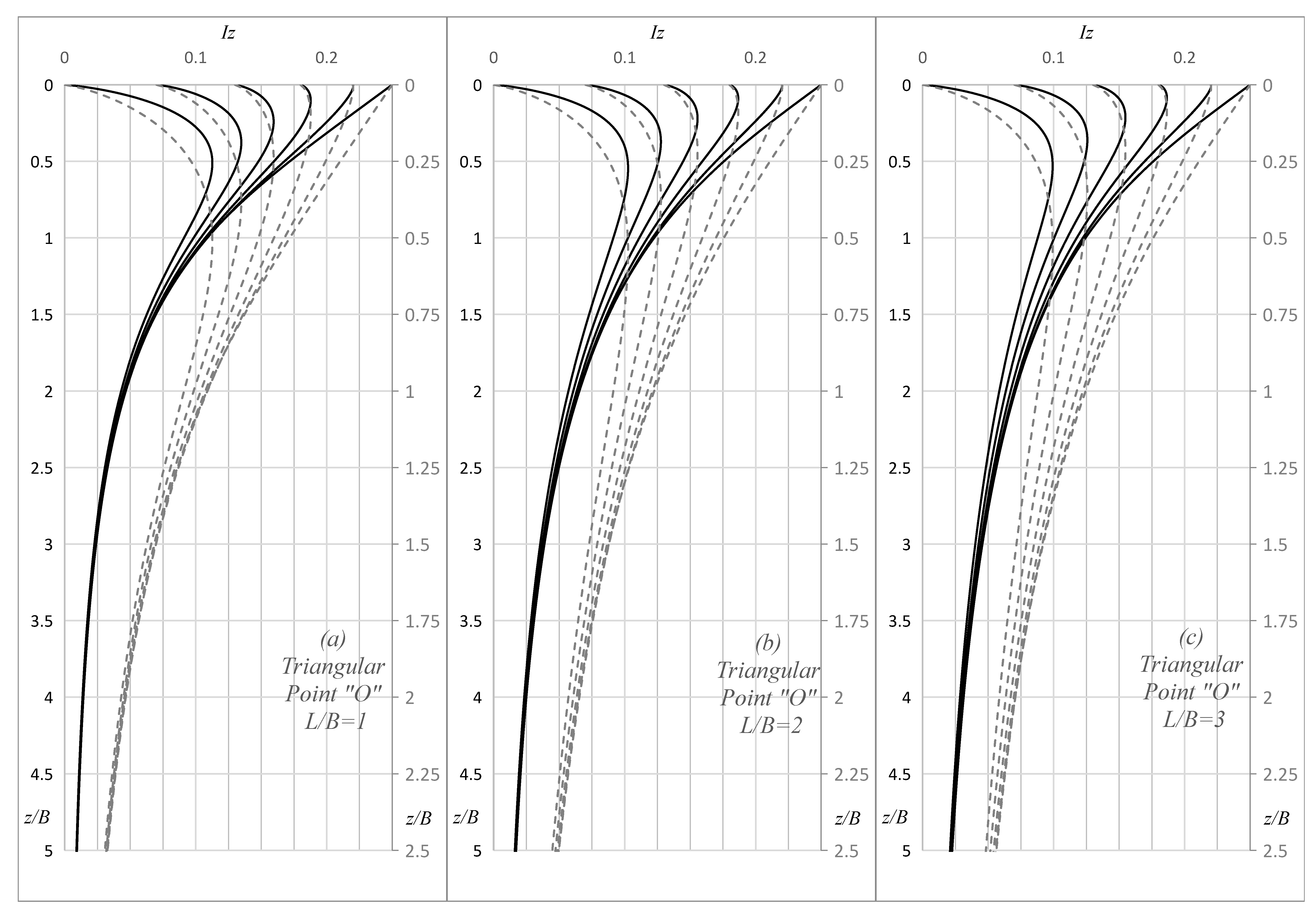
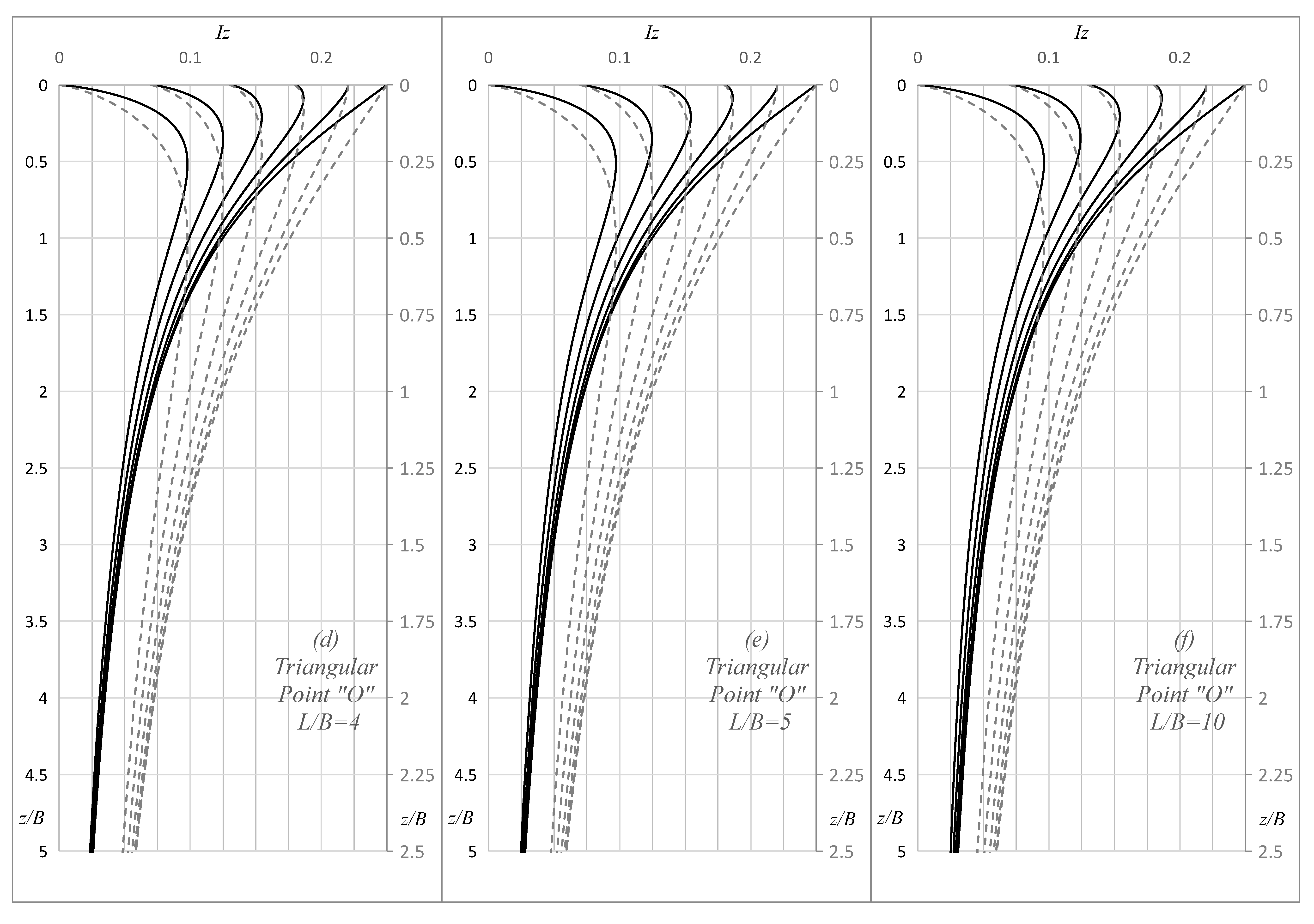
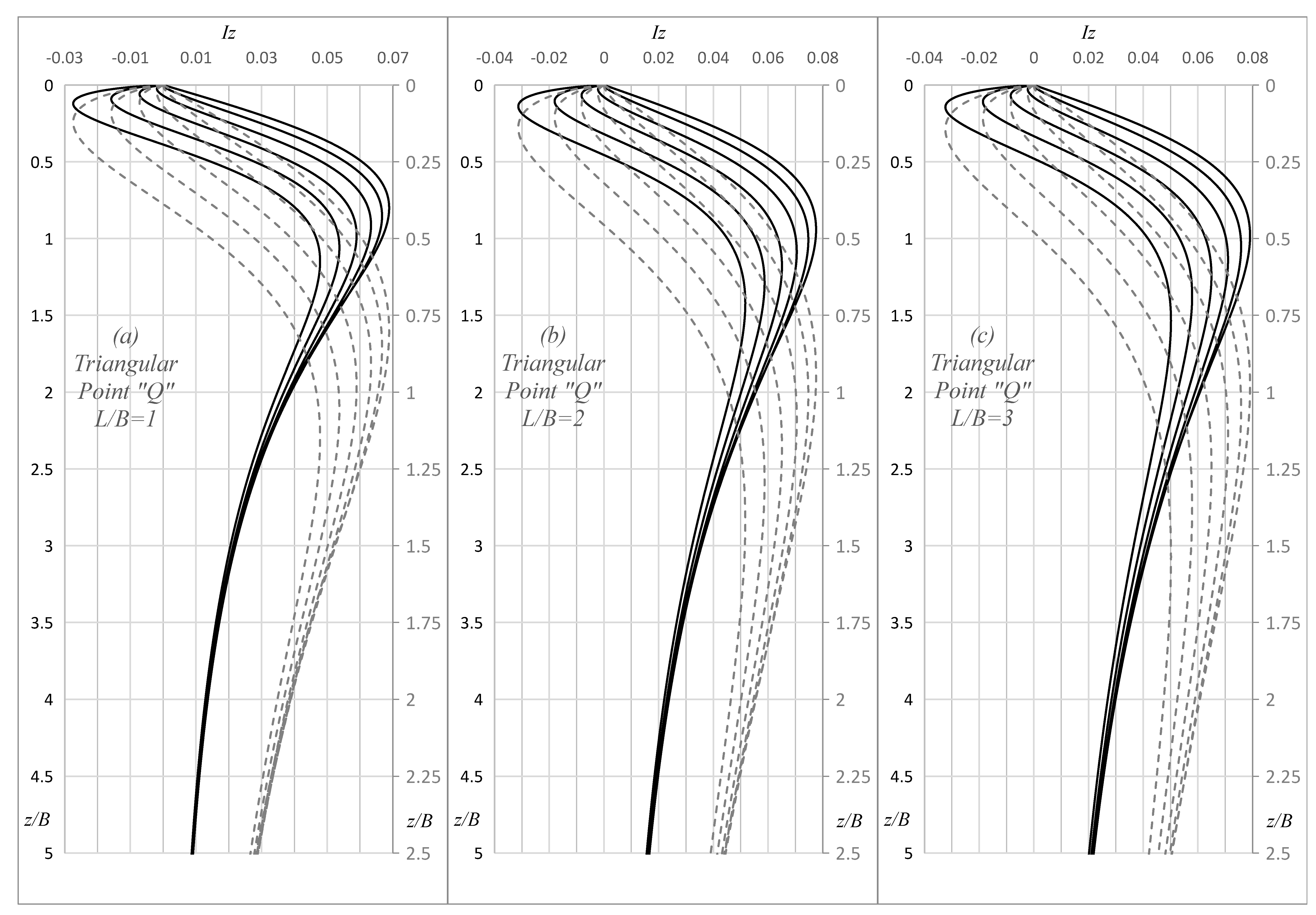
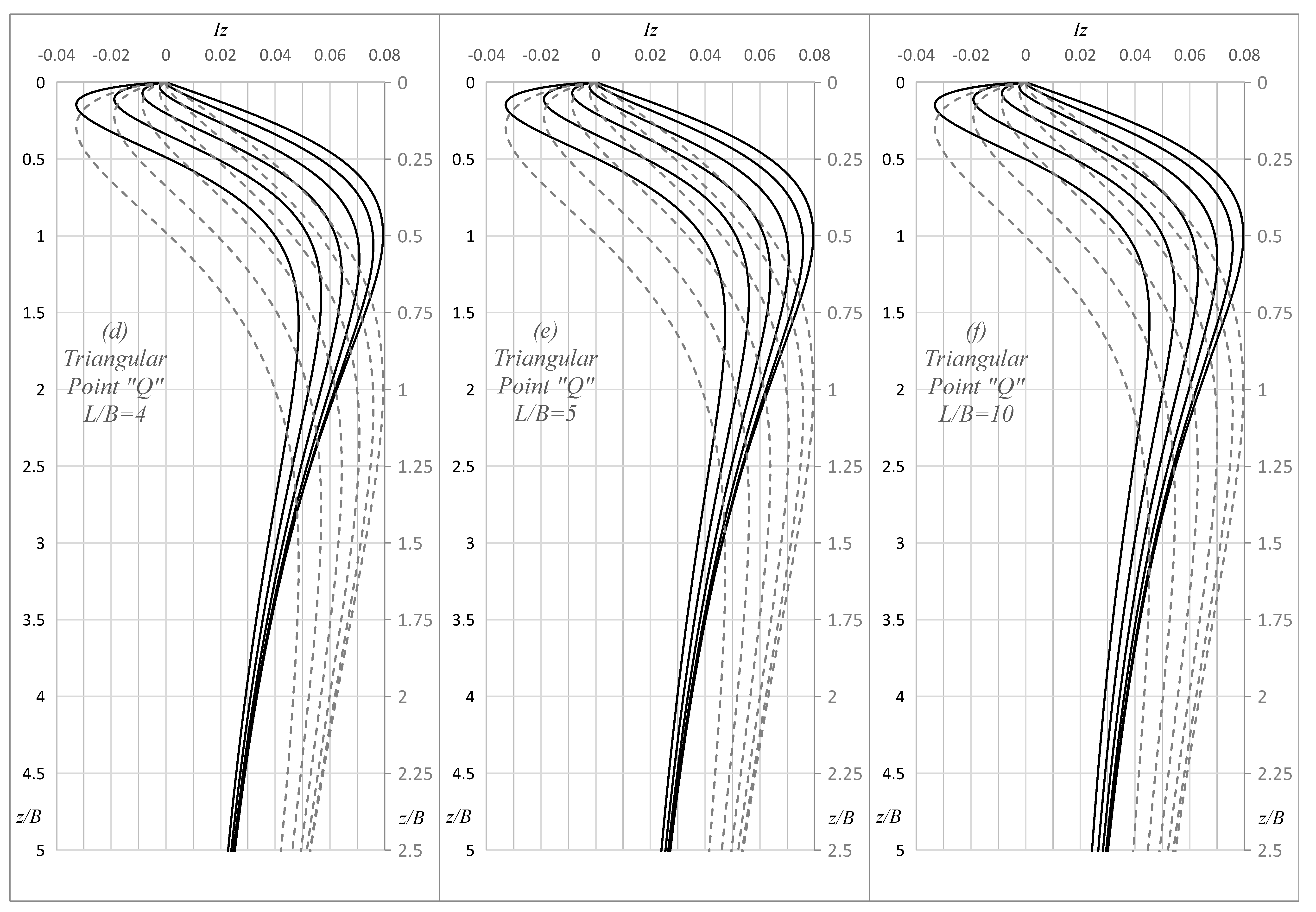
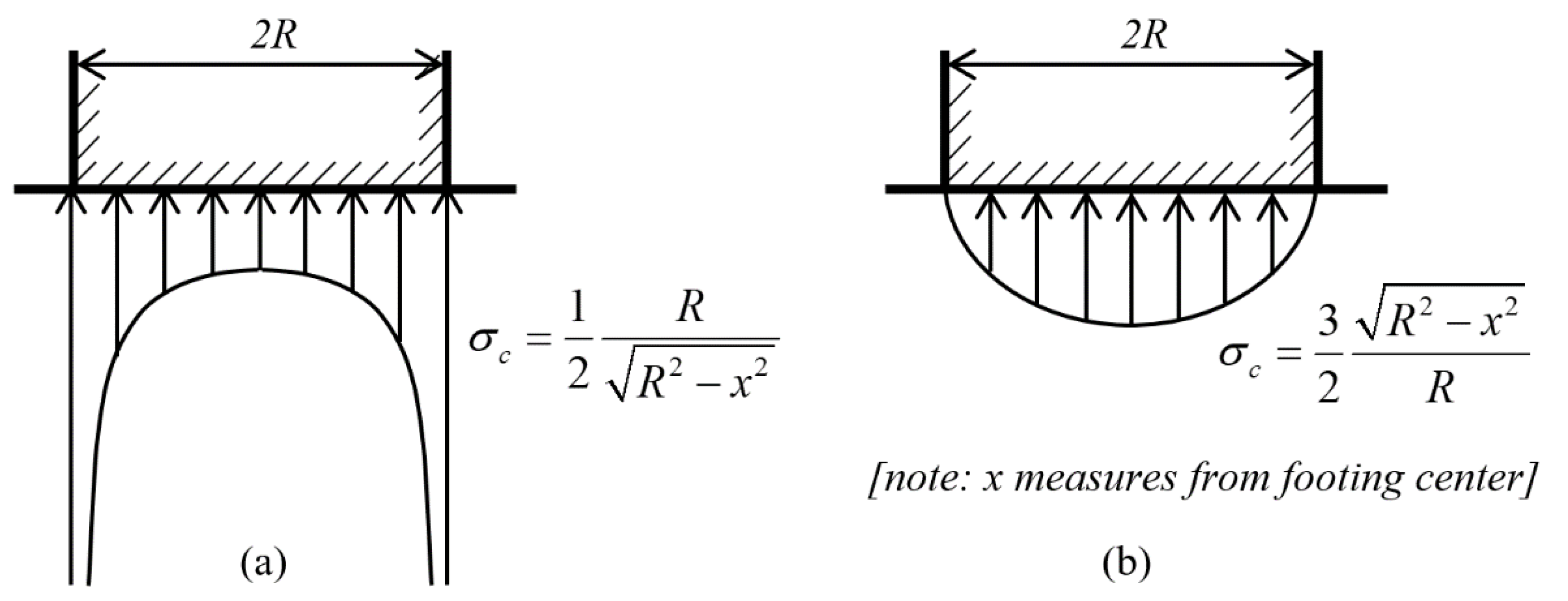
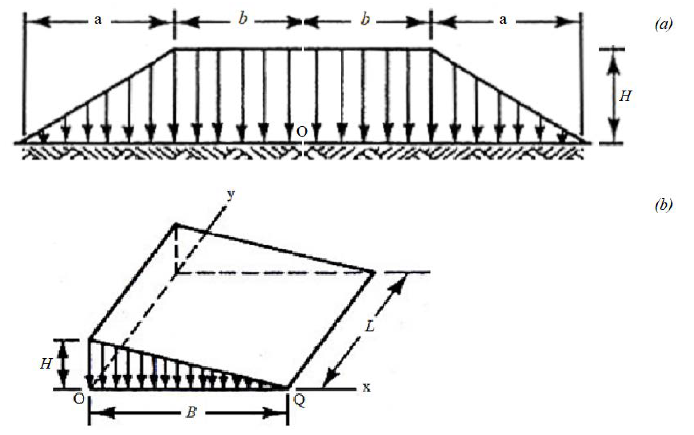
Thus, the problem is reduced to defining the proper Iz factor reflecting the shape of foundation in plan view. Using the above equations with the integration limits summarized in Table 1, the Iz versus normalized depth charts for circular and rectangular footings as well as for embankment loadings have been drawn (see Figure 2, Figure 3, Figure 4, Figure 5, Figure 6 and Figure 7). More specifically, charts (a) to (d) of Figure 2 refer to distance equal to zero (i.e. at the center), R/3, 2R/3 and R (i.e. at the perimeter) from the center of flexible circular footings, whilst charts (e) and (f) refer to rigid circular footing on clay and sand, respectively. The case of “clay” is distinguished from the case of “sand” by the contact pressure distribution; these distributions are shown in Figure 8. More specifically, a contact pressure distribution of parabolic form, where the minimum and maximum pressure value is found at the center and edges of footing, respectively, is more suitable for clays. For smooth rigid footings on clean sand, the minimum and maximum contact pressure are observed at the edges and the center of the footing, respectively [2]. Figure 3 and Figure 4 refer to the center and corner of L/B = 1, 2, 3, 4, 5 and 10 rectangular footings, respectively, where B and L are the width and length of footing. Figure 5 refers to point “O” of the symmetrical embankment shown in Figure 9. Figure 6 and Figure 7 refer to point “O” and “Q” of the triangular embankment loading of finite length shown in Figure 9.
For the two embankments of Figure 8, the loading has been expressed with respect to x as follows:
where γ and H are the unit weight of the material and the height of the embankment, respectively; x measures from the point where the settlement is calculated. The principle of superposition can be used for the calculation of the settlement at points other than “O” and “Q”. It is also noted that, in the special case of the embankment loadings, the quantity γH has been used in the denominator of Equation (7) instead of q for producing a non-dimensional Iz factor.
3. Suitability of the “Characteristic Point” Concept in a Stress–Strain Analysis Framework
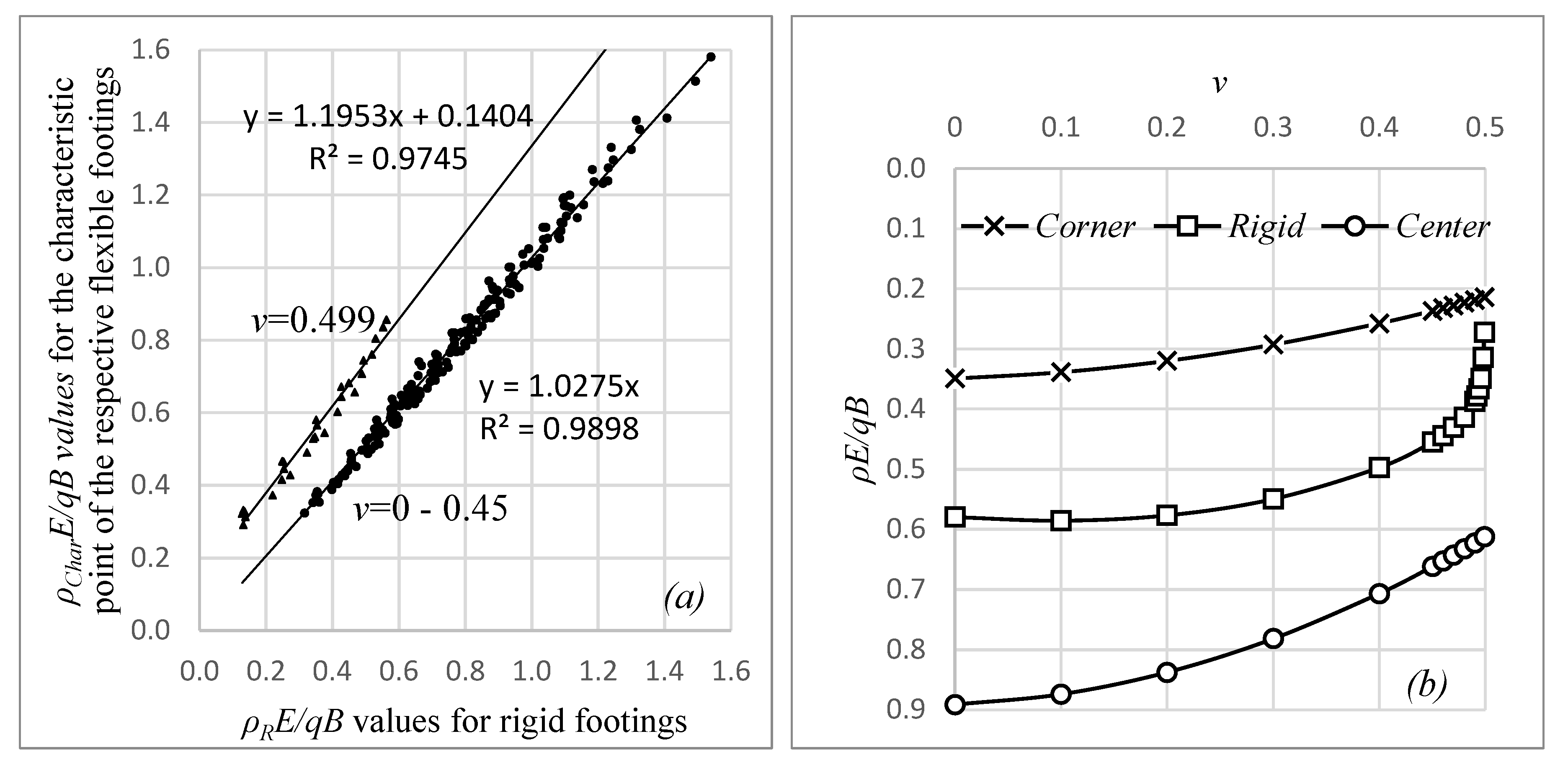
The charts of Figure 3 could be used for the calculation of the settlement of flexible rectangular footings at the so-called “characteristic point”, ρChar [27,28]. The settlement at the characteristic point of a flexible footing is considered to be the same as the uniform settlement of the respective rigid footing, ρR. According to Grasshoff [27], the characteristic point of circular footings lies at distance 0.845R from the center, whilst it lies approximately at distance 0.74B/2 and 0.74L/2 from the center of the B × L rectangular footings; B and L are the width and length of the footing, respectively, whilst R is the radius of the circular footing. As shown in Figure 10a, the settlement at the characteristic point of flexible footings effectively approximates the settlement of the respective rigid footings, but only for Poisson’s ratio values of soil smaller than 0.45. As ν approaches 0.5, an abrupt reduction in the ρΕ/qB value is observed (see Figure 10b). Such behavior is not observed for the respective ρΕ/qB values of the flexible footing. The settlement of rigid rectangular footings was calculated using the three-dimensional finite element program rsetl3d developed by Professors D.V. Griffiths and G. Fenton (the program in question is freely available at http://random.engmath.dal.ca/rfem/ [29]). In this parametric analysis, various cases were considered, i.e. rigid rectangular footings with L/B = 1, 1.8, 3.2, 5.6 and 10 over homogenous elastic medium with ν = 0, 0.1, 0.2, 0.3, 0.4, 0.45 and 0.499, and normalized thickness (H/B) of the medium in question ranging from 1 to zl/B with 0.5 interval (plus the case of 2zl/B); H is the thickness of the compressible medium. The footing width, B, was kept constant and equal to 1 m for all 210 cases analyzed. Eight-noded cubic elements of edge 0.1 m were used. The settlement at the characteristic point was calculated based on the theory of elasticity [30] using Wolfram Mathematica.
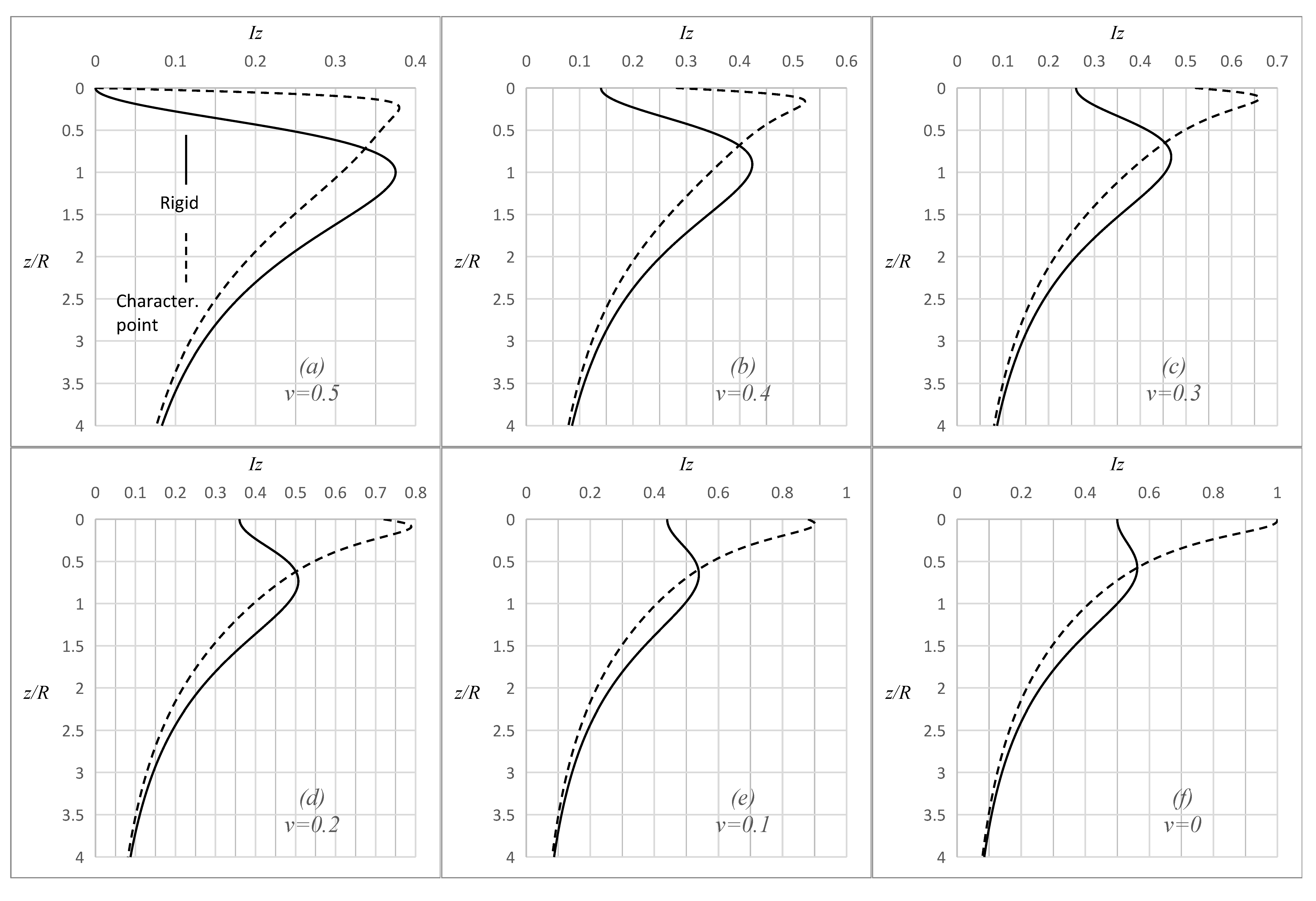
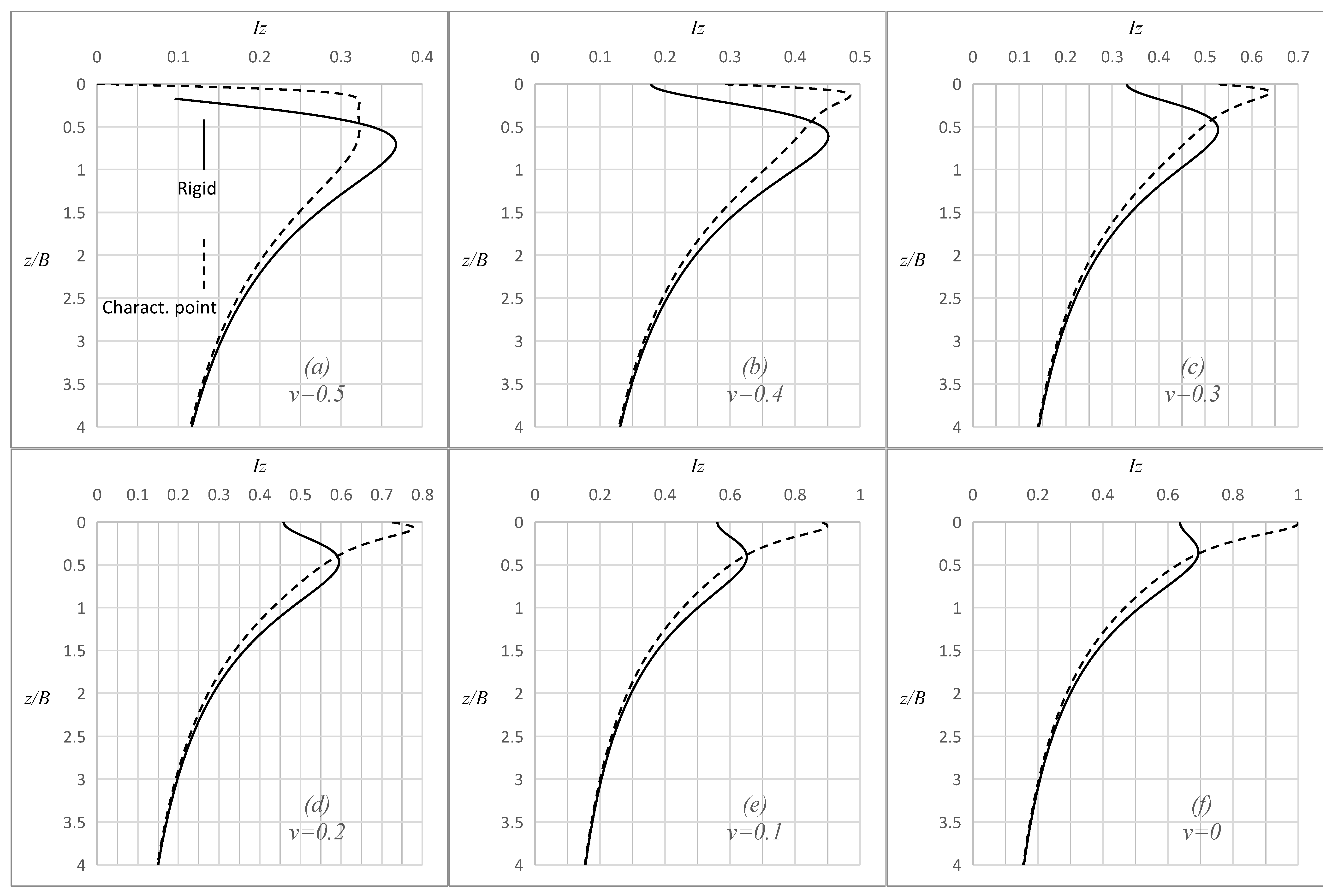
As shown in the Iz vs. normalized depth charts of Figure 11 and Figure 12 for circular and strip footings, respectively, the case of rigid footings deviates greatly from the respective one referring to flexible footings at the characteristic point and despite the fact that the areas bounded by the two curves in each chart are (approximately) equal. This means that the “characteristic point” concept, although suitable for homogenous soils (at least for ν values smaller than 0.45), is not suitable for non-homogenous soils, as it largely overestimates the settlement near the footing (for z/B < 0.35) and underestimates it at greater depths (for z/B > 0.35); B is the footing width. The contact pressure distribution used for the case of rigid circular footings is given in Figure 8a, whilst the contact pressure distribution for the case of rigid strips is given below [31]:
where b is the half width of the strip while x measures from the centerline of the stip.
4. Water Table Correction Factor for Settlement Analysis of Footings on Granular Soils
According to the literature, when the water table rises into the influence zone of footings, it reduces the soil stiffness, and thus additional settlement is induced. Several researchers attempted to quantify this phenomenon, suggesting a suitable water table correction factor, Cw [2,32,33,34,35,36,37,38]; in these studies, Cw is related to the depth of the water table measured from the foundation level (this depth defines the unsaturated zone), the embedment depth of footing and the footing width. A critical review of these approaches is out of the scope of the present paper; besides, this has already been done by Shahriar et al. [39]. Very recently, based on laboratory model tests in sands and numerical modeling, the same authors [40,41] concluded to the following expression for Cw:
where n and Cw,max are site-specific parameters depending on the relative density of sand and the shape of footing, whilst Aw and At are areas on the influence factor diagram corresponding to the “submerged” and total area, respectively (apparently up to the influence depth of footing). Shahriar et al. [40] suggested that Cw,max be determined by model tests, measuring the additional settlement induced after inundating the entire sand; generally, the Cw,max is greater in loose sands. n, also according to Shahriar et al. [40], can be assumed as unity for all practical purposes, especially as a first estimate. Das [42] suggests that Equation (11) be simplified as follows:
Adopting either Equation (11) or Equation (12), the strain influence factor charts presented herein can be used for determining the areas Aw and At. The updated settlement value derives, finally, from the multiplication of ρ given by Equation (8) with Cw.
It is noted that this correction is not necessary if the soils’ elastic modulus is taken from relations with the probing test data (e.g., CPT, SPT). However, if for any reason the water table were to rise into or above the zone of influence zl after the penetration tests were conducted, this correction is necessary for the soil layers, being between the initial and new water table level (see also [2,43,44]).
At this point, the author would like to mention that various researchers express the opinion that the degree of saturation has only a minor effect on the qc value of the CPT test [45,46,47,48,49] and in turn, on the elastic modulus of soil and the settlement of footing. Other researchers (e.g., [50]) observed that qc is influenced to a great extent by the water table depth (due to suction), so that qc increases.
5. Discussion
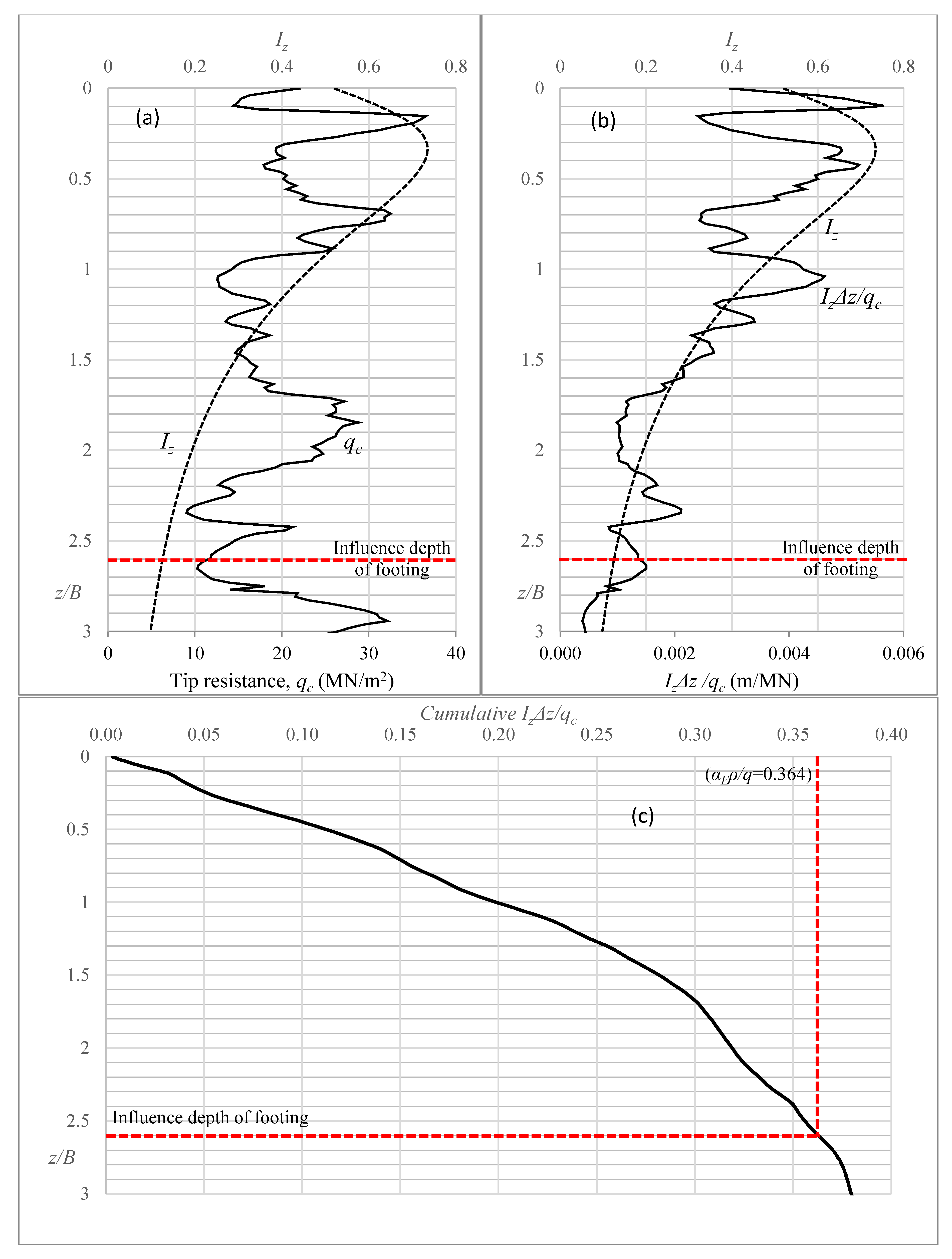
The discussion herein is facilitated through an application example. Let there be a flexible rectangular footing with B = 2.6 m and L/B = 2. The footing is founded on the surface of a soil medium for which the tip resistance (qc) of the CPT apparatus is known; see the qc–z/B chart in Figure 13a. The qc value is available every 0.05 m (that is, Δz = 0.05 m). Poisson’s ratio of soil is ν = 0.3 (assumed to be the same throughout the soil mass). The Iz–z/B curve for the Poisson’s value in question has also been drawn on the same chart (curve also appearing in Figure 3b). This curve is effectively represented (R2 = 0.9999) by the following polynomial (MS Office Excel was used):
The Iz–z/B curve for any ν value can easily be reproduced using an adequate number of points in a spreadsheet. Additionally, if the soil mass consists of successive layers with different ν values, the Iz–z/B curve corresponding to the correct ν value should be used for each layer.
The elastic modulus of soil is often obtained from soil probing tests (e.g., CPT or SPT) relying on an empirical relationship. Indeed, tens of such relationships correlating probe test parameters with E exist in literature (e.g., [4,24,51,52,53,54,55,56]. The most common forms of these relationships referring to the CPT and SPT tests are summarized below:
where and are empirical coefficients, is the number of blows required for 12 inches penetration resistance of the soil, is the vertical geostatic stress and is the corrected cone resistance. The coefficients and are site-specific and depend on the type and relative density of the soil and whether the soil is normally consolidated or overconsolidated, as well as whether it is saturated or not. In the present example, an empirical correlation of the form has been used. Therefore, for the example examined herein, Equation (8) can be rewritten as follows:
According to Terzaghi et al. [2], the influence depth of footing is approximately equal to ; in this respect, 2.6B. The IzΔz/qc–z/B chart is given in Figure 13b for z/B up to 3B, giving, in essence, the contribution of each soil substratum of thickness Δz to the settlement of footing. The cumulative IzΔz/qc values with respect to z/B are given in Figure 13c. z/B is the depth in normalized form.
The footing shape is also known to affect the modulus of elasticity of soil and, in turn, the elastic settlement of footing. For considering the effect of the footing shape on the elastic settlement, Schmertmann et al. [24] and later Terzaghi et al. [2] adopted Lee’s [57] Ep/Et = 1.4 relationship between the axisymmetric and the plane strain loading case (Et and Ep are the triaxial and plane strain moduli, respectively; the validity of Lee’s relationship is discussed by the author in in [11]). In this respect, Terzaghi et al. suggested the following interpolation function:
Apparently this value is smaller than the constrained modulus of soil [60], also known as the oedometer modulus.
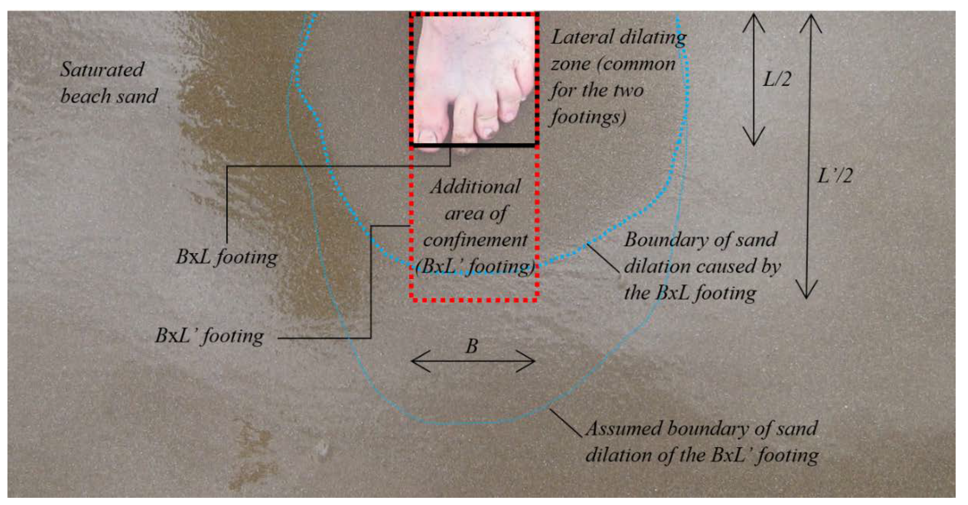
This produces the very interesting observation that the empirical correction for the modulus of elasticity of soil of Equation (17) seems to cancel out the adverse effect of the second (long) dimension of footing on the elastic settlement [58]. This is due to the extra confinement offered by the longer footing. The confinement, as can be observed on the surface of saturated beach sand, is indicated in Figure 14. It is mentioned that the general mechanism of the embedment depth is very similar, which however acts around the perimeter of footing whilst its effect depends on the weight of the surrounding soil mass, γDf (embedment correction factors have been suggested by [1,2,20,43,61,62,63,64]). Thus, for the example examined here, Equation (15) becomes:
Ignoring the empirical correction of Equation (17), the problem is reduced to finding the settlement of the respective B × B footing, or better, the settlement of a circular footing having an equivalent diameter equal to [58]. However, because the influence depth of the circular footing is smaller, the analysis should be based on a homogenous soil medium having equivalent elastic constants; such an equivalent medium effectively reflects the influence of all soil strata up to the influence depth of the original B × L footing [65]. According to the author [65], this can be found by equating the derived settlement (without the footing shape correction mentioned above) with the settlement derived from elastic theory (Steinbrenner’s [30] or Harr’s [66] solutions can be used). In this respect, Steinbrenner’s [30] solution will be used. For the center of the footing, this has the form:
where is a dimensionless factor taking into account the shape of footing and the thickness and Poisson’s ratio of the compressible stratum, i.e., = . is the thickness of the compressible stratum or the influence depth of footing (whichever of the two is smaller). More specifically,
with
(=2) and (= 2∙2.6 = 5.2).
From Equations (15) and (17) and for an influence depth of footing equal to 2.6B (i.e., 6.76 m):
The latter is solved as for ,
where is also unknown. According to Pantelidis [65], however, any equivalent elastic constant pair of values satisfying Equation (26) not only returns the same maximum settlement value (as expected) but also produces the same settlement profile. Adopting Schmertmann’s [24] = 2 value for illustrating purposes, the denominator in Equation (26) equals 0.182 m/MPa (recall Figure 13c). Assume, now, that νeq = 0, Is = 0.591 and thus Eeq = 16.89 MPa. If νeq = 0.3, Is = 0.567 and, thus, Eeq = 14.74 MPa. Both solutions (i.e., {16.89, 0}, {14.74, 0.3}) are correct as, as mentioned, they produce the same settlement profile. More specifically, from Figure 13c the settlement per unit loading (ρ/q) if = 2 is 0.182 m/MPa. Using Steinbrenner’s formula with the equivalent elastic parameters, the ρ/q ratio is also equal to 0.182 for both Eeq = 16.89 MPa, νeq = 0 and Eeq = 14.74 MPa, νeq = 0.3 pair of values.
Applying the correction for the footing shape of Equation (17), the ρ/q ratio becomes equal to 0.182/1.3 = 0.140 m/MPa. For the respective square footing with an edge B = 2.6 m and influence depth equal to 2B, the ρ/q ratio using Steinbrenner’s formula is 0.138 m/MPa (no correction is needed). Thus, the same settlement is obtained.
Since the settlement of a square footing is approximately equal to the respective circular footing having the same area on plan view (that is, having a diameter ), the settlement of the B × L rectangular footing could be calculated based on the respective circular footing with the use of the equivalent elastic constants of soil and ignoring the correction for footing shape. The following analytical expressions could be used for rigid circular footings on clay and sand:
For completeness, the settlement at the center of flexible circular footing, which rather corresponds to footing on clay soil, is:
As H∞, the term in the square brackets in Equations (27) to (29) tends to unity, thus:
Thus, from Equation (29) using R = = 1.47 m, H = 4R = 5.87 m and the equivalent elastic constants, the ρ/q ratio is 0.142 m/MPa, that is, approximately equal to the 0.138 m/MPa value obtained previously. If the B × L footing considered in this example was rigid and on the surface of clay or sand, the ρ/q ratio would be 0.105 and 0.173 m/MPa using Equations (27) and (28) respectively. It is reminded that, for comparison purposes, the two materials share the same elastic modulus value.
Finally, it is mentioned that the Eeq = 16.89 MPa, which stands for νeq = 0, is the proper value for use in a Winkler spring type of analysis, as a Poisson’s ratio value equal to zero better represents the deformation pattern of springs.
6. Summary and Conclusions
In this paper, the problem of calculating the elastic settlement of footings relying on the stress–strain method has been revisited, offering a great number of strain influence factor charts covering the most common cases met in civil engineering practice. The calculation of settlement based on strain influence factors has the advantage of considering elastic moduli values rapidly varying with depth and also the convenient calculation of the correction factor for future water table rise into the influence depth of footing. As known, when the water table rises into the influence zone of footing, it reduces the soil stiffness, and thus additional settlement is induced. The proposed factors refer to flexible circular footings (at distances 0, R/3, 2R/3 and R from the center; R is the radius of footing), rigid circular footings, flexible rectangular footings (at the center and at the corner), triangular embankment loading of width B and length L (L/B = 1, 2, 3, 4, 5 and 10) and trapezoidal embankment loading of infinite length and various widths. The strain influence factor values are given for a Poisson’s ratio value ranging from 0 to 0.5 with 0.1 interval.
The compatibility of the so-called “characteristic point” of flexible footings with the stress–strain method has also been investigated. The study of settlement values from 210 different cases of rigid footings on homogenous medium (values derived from 3D finite element analysis) showed that the characteristic point concept is highly reliable but only for an analysis under drained conditions. Despite of the effectiveness of the “characteristic point” concept in homogenous soils, the method in question is not suitable for non-homogenous soils, as it largely overestimates settlement near the footing (for z/B < 0.35) and underestimates it at greater depths (for z/B > 0.35; z is the depth and B is the footing width).
The proposed charts can also be used for replacing the original non-homogeneous medium with a homogenous one having equivalent elastic constant values. The equivalent homogenous medium gives the same settlement profile as the original one. This is an intermediate step for calculating the settlement of rigid rectangular footings on sands or clays based on the settlement of the respective circular footing. The reduction of the problem of a B × L footing to the problem of the respective circular one is possible due to the effect of the shape of footing on the elastic modulus of soil. Finally, the equivalent elastic modulus corresponding to a Poisson’s ratio value equal to zero can also be obtained. This value is of particular importance, as this is the proper value for use in a Winkler spring type of analysis as a Poisson’s ratio value equal to zero better represents the deformation pattern of springs.
Funding
This research received no external funding.
Acknowledgments
The author would like to cordially thank Panagiotis Christodoulou for his help in running the finite element models.
Conflicts of Interest
The author declares no conflicts of interest.
References
- Schmertmann, J.H.; Hartman, J.P.; Brown, P.R. Improved strain influence factor diagrams. J. Geotech. Geoenviron. Eng. 1978, 104, 1131–1135. [Google Scholar]
- Terzaghi, K.; Peck, R.B.; Mesri, G. Soil Mechanics in Engineering Practice; John Wiley: New York, NY, USA, 1996; ISBN 0471086584. [Google Scholar]
- Lunne, T.; Robertson, P.K.; Powell, J.J.M. Cone-penetration testing in geotechnical practice. Soil Mech. Found. Eng. 2009, 46, 237. [Google Scholar] [CrossRef] [Green Version]
- Coduto, D.P. Foundation Design: Principles and Practices, 2nd ed.; Prentice Hall: Upper Saddle River, NJ, USA, 2001; ISBN 978-0133411898. [Google Scholar]
- Salgado, R. The Engineering of Foundations; McGraw-Hill: New York, NY, USA, 2008; Volume 888, ISBN 978-0072500585. [Google Scholar]
- Lee, J.; Eun, J.; Prezzi, M.; Salgado, R. Strain influence diagrams for settlement estimation of both isolated and multiple footings in sand. J. Geotech. Geoenviron. Eng. 2008, 134, 417–427. [Google Scholar] [CrossRef]
- Barksdale, R.D.; Blight, G.E. Compressibility, settlement and heave of residual soils. In Mechanics of Residual Soils; Blight, G.E., Leong, E.., Eds.; CRC Press: Boca Raton, FL, USA, 2012; pp. 149–212. [Google Scholar]
- CEN. EN 1997-2: Geotechnical Design—Part 2: Ground Investigation and Testing; European Committee for Standardization: Brussels, Belgium, 2007; ISBN 0580 24511X. [Google Scholar]
- AASHTO. AASHTO LRFD Bridge Design Specifications; American Association of State Highway and Transportation Officials: Washington, DC, USA, 2010; ISBN 9781560514510. [Google Scholar]
- Samtani, N.C.; Nowatzki, E.A. Soils and Foundations—Volumes I and II. Publications No. FHWA NHI-06-088 and FHWA NHI-06-089; Federal Highway Administration: Washington, DC, USA, 2006. [Google Scholar]
- Pantelidis, L. A Critical Review of Schmertmann’s Strain Influence Factor Method for Immediate Settlement Analysis. Geotech. Geol. Eng. 2020, 38, 1–18. [Google Scholar] [CrossRef]
- Briaud, J.-L.; Gibbens, R. Large-Scale Load Tests and Data base of Spread Footings on Sand; United States. Federal Highway Administration: Washington, DC, USA, 1997. [Google Scholar]
- Briaud, J.-L.; Gibbens, R. Behavior of five large spread footings in sand. J. Geotech. Geoenviron. Eng. 1999, 125, 787–796. [Google Scholar] [CrossRef]
- Gifford, D.G.; Kraemer, S.R.; Wheeler, J.R.; McKown, A.F. Spread Footings for Highway Bridges; Final Report (No. FHWA/RD-86/185); Federal Highway Administration: Cambridge, MA, USA, 1987. [Google Scholar]
- Tan, C.K.; Duncan, J.M. Settlement of footings on sands—Accuracy and reliability. In Proceedings of the Geotechnical Engineering Congress, Boulder, CO, USA, 10–12 June 1991; ASCE: Reston, VA, USA, 1991; pp. 446–455. [Google Scholar]
- Anderson, D.G. Seismic Analysis and Design of Retaining Walls, Buried Structures, Slopes, and Embankments; Transportation Research Board: Washington, DC, USA, 2008; Volume 611, ISBN 0309117658. [Google Scholar]
- Ahmed, A.Y. Reliability Analysis of Settlement for Shallow Foundations in Bridges; University of Nebraska: Lincoln, NE, USA, 2013. [Google Scholar]
- Birid, K.C.; Chahar, R.S. Measured and Predicted Settlement of Shallow Foundations on Cohesionless Soil. In Geotechnical Applications; Anirudhan, I.V., Maji, V.B., Eds.; Springer: Singapore, 2019; pp. 3–13. ISBN 978-981-13-0368-5. [Google Scholar]
- Maugeri, M.; Castelli, F.; Massimino, M.R.; Verona, G. Observed and computed settlements of two shallow foundations on sand. J. Geotech. Geoenviron. Eng. 1998, 124, 595–605. [Google Scholar] [CrossRef]
- Mayne, P.W.; Poulos, H.G. Approximate displacement influence factors for elastic shallow foundations. J. Geotech. Geoenviron. Eng. 1999, 125, 453–460. [Google Scholar] [CrossRef]
- Tatsuoka, F.; Teachavorasinskun, S.; Dong, J.; Kohata, Y.; Sato, T. Importance of Measuring Local Strains in Cyclic Triaxial Tests on Granular Materials. In STP1213-EB Dynamic Geotechnical Testing II; Ebelhar, R., Drnevich, V., Kutter, B., Eds.; ASTM International: West Conshohocken, PA, USA, 1994; pp. 288–302. [Google Scholar]
- Jamiolkowski, M.; Lancellotta, R.; LoPresti, D.C.F. Remarks on the stiffness at small strains of six Italian clays. In Proceedings of the International Symposium on Pre-failure Deformation Characteristics of Geomaterials, Sapporo, Japan, 12–14 September 1994; Shibuya, S., Mitachi, T., Miura, S., Eds.; Balkema: Rotterdam, The Netherlands, 1995; Volume 2, pp. 817–836. [Google Scholar]
- Shahriar, M.A.; Sivakugan, N.; Das, B.M. Strain Influence Factors for Footings on an Elastic Medium. In Proceedings of the 11th Australia—New Zealand Conference on Geomechanics, Ground Engineering in a Changing World, Crown Conference Centre, Melbourne, Australia, 15–18 July 2012; Narsilio, G.A., Australian Geomechanics Society, New Zealand Geotechnical Society, Eds.; Australian Geomechanics Society and the New Zealand Geotechnical Society: Melbourne, Australian, 2012; pp. 131–136. [Google Scholar]
- Schmertmann, J.H. Static cone to compute static settlement over sand. J. Soil Mech. Found. Div. 1970, 96, 1011–1043. [Google Scholar]
- Boussinesq, J. Application des Potentiels à l’étude de l’équilibre et du Mouvement des Solides élastiques: Principalement au Calcul des Déformations et des Pressions que Produisent, Dans Ces Solides, des Efforts Quelconques Exercés sur une Petite Partie de Leur Surface; Forgotten Books: Paris, France, 1885; ISBN 978-0243352630. [Google Scholar]
- Das, B.M. Fundamentals of Geotechnical Engineering, 3rd ed.; CL-Engineering: Madrid, Spain, 2007; ISBN 978-0-495-29572-3. [Google Scholar]
- Grasshoff, H. Setzungsberechnungen starrer Fundamente mit Hilfe des kennzeichnenden Punktes. Bauingenieur 1955, 30, 53–54. [Google Scholar]
- Kany, M. Berechnung von Flächengründungen, 2nd ed.; Ernst u. Sohn: Berlin, Germany, 1974. [Google Scholar]
- Fenton, G.A.; Griffiths, D.V. Three-Dimensional Probabilistic Foundation Settlement. J. Geotech. Geoenviron. Eng. 2005, 131, 232–239. [Google Scholar] [CrossRef] [Green Version]
- Steinbrenner, S.W. Tafeln zur setzungsberechnung. Die StraBe 1934, 1, 121–124. [Google Scholar]
- Kézdi, A.; Rétháti, L. Volume 3: Soil Mechanics of Earthworks, Foundations and Highway Engineering, Handbook of Soil Mechanics; Elsevier: New York, NY, USA, 1988; ISBN 0-444-98929-3. [Google Scholar]
- Teng, W.C. Foundation Design; Prendice-Hall INc.: New York, NY, USA, 1962. [Google Scholar]
- Alpan, I. Estimating the settlements of foundations on sands. Civ. Eng. Public Work Rev. 1964, 59, 1415–1418. [Google Scholar]
- Bazaraa, A.R. Use of the Standard Penetration Test for Estimating Settlements of Shallow Foundations on Sand; University Microfilms: Ann Arbor, MI, USA, 1967. [Google Scholar]
- Bowles, L.E. Foundation Analysis and Design, 5th ed.; McGraw-hill: Singapore, 1996; ISBN 0079122477. [Google Scholar]
- Peck, R.B.; Hanson, W.E.; Thornburn, T.H. Foundation Engineering, 2nd ed.; John Willy & Sons: New York, NY, USA, 1974; ISBN 978-0-471-67585-3. [Google Scholar]
- Agarwal, K.B.; Rana, M.K. Effect of ground water on settlement of footings in sand. In Proceedings of the European Conference on Soil Mechanics and Foundation Engineering, Dublin, Ireland, 31 August–3 September 1987; Hanrahan, E.T., Orr, T.L.L., Widdis, T.F., Eds.; A.A. Balkema: Rotterdam, The Netherlands, 1987; Volume 9, pp. 751–754. [Google Scholar]
- NAVFAC. Soil Mechanics Design Manual (NAVFAC DM 7.1); Naval Facilities Engineering Command: Alexandria, VA, USA, 1982. [Google Scholar]
- Shahriar, M.; Sivakugan, N.; Das, B. Settlements of shallow foundations in granular soils due to rise of water table—A critical review. Int. J. Geotech. Eng. 2012, 6, 515–524. [Google Scholar] [CrossRef]
- Shahriar, M.A.; Sivakugan, N.; Das, B.M.; Urquhart, A.; Tapiolas, M. Water Table Correction Factors for Settlements of Shallow Foundations in Granular Soils. Int. J. Geomech. 2015, 15, 06014015. [Google Scholar] [CrossRef]
- Shahriar, M.A.N.; Sivakugan, N.; Das, B.M. Settlement correction for future water table rise in granular soils: A numerical modelling approach. Int. J. Geotech. Eng. 2013, 7, 214–217. [Google Scholar] [CrossRef]
- Das, B.M. Shallow Foundations: Bearing Capacity and Settlement, 3rd ed.; CRC Press: Boca Raton, FL, USA, 2017; ISBN 9781315163871. [Google Scholar]
- Burland, J.; Burbidge, M.; Wilson, E. Settlement of foundations on sand and gravel. Proc. Inst. Civ. Eng. 1985, 78, 1325–1381. [Google Scholar] [CrossRef]
- Meyerhof, G.G. Shallow foundations. J. Soil Mech. Found. Div 1965, 91, 21–31. [Google Scholar]
- Jamiolkowski, M.; Lo Presti, D.C.F.; Manassero, M. Evaluation of Relative Density and Shear Strength of Sands from CPT and DMT. In Proceedings of the Soil Behavior and Soft Ground Construction, Cambridge, MA, USA, 5–6 October 2001; American Society of Civil Engineers: Reston, VA, USA, 2003; pp. 201–238. [Google Scholar]
- Bellotti, R.; Crippa, V.; Pedroni, S.; Ghionna, V.N. Saturation of sand specimen for calibration chamber tests. In Proceedings of the International Symposium on Penetration Testing, Orlando, FL, USA, 20–24 March 1988; pp. 661–671. [Google Scholar]
- Villet, W.C.B.; Mitchell, J.K. Cone resistance, relative density and friction angle. In Proceedings of the Cone penetration Testing and Experience, St. Louis, MO, USA, 26–30 October 1981; ASCE: New York, NY, USA, 1981; pp. 178–208. [Google Scholar]
- Bonita, J.A. The Effects of Vibration on the Penetration Resistance and Pore Water Pressure in Sands. Ph.D. Thesis, Virginia Tech, Blacksburg, VA, USA, 2000. [Google Scholar]
- Schmertmann, J.H. An Updated Correlation between Relative Density, Dr, and Fugro-type Electric Cone Bearing, qc (Report DACW 39-76 M6646); Waterway Experimental Atation: Vicksburg, MS, USA, 1976. [Google Scholar]
- Lo Presti, D.; Stacul, S.; Meisina, C.; Bordoni, M.; Bittelli, M. Preliminary Validation of a Novel Method for the Assessment of Effective Stress State in Partially Saturated Soils by Cone Penetration Tests. Geosciences 2018, 8, 30. [Google Scholar] [CrossRef] [Green Version]
- Rao, N.S.V.K. Foundation Design: Theory and Practice; John Wiley & Sons: Singapore, 2010; ISBN 0470828153. [Google Scholar]
- Fang, H.-Y. Foundation Engineering Handbook, 2nd ed.; Springer: New York, NY, USA, 1991; ISBN 1475752717. [Google Scholar]
- Canadian Geotechnical Society. Canadian Foundation Engineering Manual, 4th ed.; Canadian Geotechnical Society: Edmonton, AB, Canada, 2006. [Google Scholar]
- Sanglerat, G. The Penetrometer and Soil Exploration; Elsevier: New York, NY, USA, 1972; ISBN 0444599363. [Google Scholar]
- Murthy, V.N.S. Geotechnical Engineering: Principles and Practices of Soil Mechanics and Foundation Engineering; Marcel Dekker: New York, NY, USA, 2002; ISBN 1482275856. [Google Scholar]
- Robertson, P.K. Interpretation of cone penetration tests—A unified approach. Can. Geotech. J. 2009, 46, 1337–1355. [Google Scholar] [CrossRef] [Green Version]
- Lee, K.L. Comparison of plane strain and triaxial tests on sand. J. Soil Mech. Found. Div. 1970, 96, 901–923. [Google Scholar]
- Pantelidis, L. Elastic Settlement Analysis for Various Footing Cases Based on Strain Influence Areas. Geotech. Geol. Eng. 2020. [Google Scholar] [CrossRef]
- Pantelidis, L. The effect of footing shape on the elastic modulus of soil. In Proceedings of the 2nd Conference of the Arabian Journal of Geosciences (CAJG), Sousse, Tunisia, 25–28 November 2019; Springer: Heidelberg, Germany, 2019. [Google Scholar]
- Poulos, H.G.; Davis, E.H. Elastic Solutions for Soil and Rock Mechanics; John Wiley & Sons: New York, NY, USA, 1991; ISBN 0471695653. [Google Scholar]
- Fox, L. The mean elastic settlement of a uniformly loaded area at a depth below the ground surface. In Proceedings of the 2nd International Conference on Soil Mechanics and Foundation Engineering, Rotterdam, The Netherlands, 21–30 June 1948; Volume 1, pp. 129–132. [Google Scholar]
- Díaz, E.; Tomás, R. Revisiting the effect of foundation embedment on elastic settlement: A new approach. Comput. Geotech. 2014, 62, 283–292. [Google Scholar] [CrossRef]
- Janbu, N.; Bjerrum, L.; Kjaernsli, B. Veiledning Ved Losing av Fandamenteringsoppgaver. Nor. Geotech. Inst. 1956, 16. [Google Scholar]
- Christian, J.; Carrier, D. Janbu, Bjerrum and Kjaernsli’s chart reinterpreted. Can. Geotech. J. 1978, 15, 123–128. [Google Scholar] [CrossRef]
- Pantelidis, L. On the modulus of subgrade reaction for shallow foundations on homogenous or stratified mediums. In Proceedings of the 3rd International Structural Engineering and Construction Conference (EURO-MED-SEC-03), Limassol, Cyprus, 3–8 August 2020; Vacanas, Y., Danezis, C., Yazdani, S., Singh, A., Eds.; ISEC Press: Limassol, Cyprus, 2020. [Google Scholar]
- Harr, M.E. Foundations of Theoretical Soil Mechanics; McGraw-Hill: New York, NY, USA, 1966; ISBN 978-0070267411. [Google Scholar]
Figure 1.
Stresses in an elastic medium caused by a point load acting on the surface of a semi-infinite mass.
Figure 1.
Stresses in an elastic medium caused by a point load acting on the surface of a semi-infinite mass.

Figure 2.
Iz versus normalized depth charts for various ν values for circular footings; ν ranges from 0.5 to 0 (left to right) with 0.1 interval.
Figure 2.
Iz versus normalized depth charts for various ν values for circular footings; ν ranges from 0.5 to 0 (left to right) with 0.1 interval.


Figure 3.
Iz versus normalized depth charts referring to the center of flexible rectangular footings for various ν values; ν ranges from 0.5 to 0 (left to right) with 0.1 interval.
Figure 3.
Iz versus normalized depth charts referring to the center of flexible rectangular footings for various ν values; ν ranges from 0.5 to 0 (left to right) with 0.1 interval.


Figure 4.
Iz versus normalized depth charts referring to the corner of flexible rectangular footings for various ν values; ν ranges from 0.5 to 0 (left to right) with 0.1 interval.
Figure 4.
Iz versus normalized depth charts referring to the corner of flexible rectangular footings for various ν values; ν ranges from 0.5 to 0 (left to right) with 0.1 interval.


Figure 5.
Iz versus normalized depth charts referring to point “O” of the symmetrical embankment loading of Figure 8a for various ν values; ν ranges from 0.5 to 0 (left to right) with 0.1 interval.
Figure 5.
Iz versus normalized depth charts referring to point “O” of the symmetrical embankment loading of Figure 8a for various ν values; ν ranges from 0.5 to 0 (left to right) with 0.1 interval.


Figure 6.
Iz versus normalized depth charts referring to point “O” of the triangular embankment loading of Figure 8b for various ν values; ν ranges from 0.5 to 0 (left to right) with 0.1 interval.
Figure 6.
Iz versus normalized depth charts referring to point “O” of the triangular embankment loading of Figure 8b for various ν values; ν ranges from 0.5 to 0 (left to right) with 0.1 interval.


Figure 7.
Iz versus normalized depth charts referring to point “Q” of the triangular embankment loading of Figure 8b for various ν values; ν ranges from 0.5 to 0 (left to right) with 0.1 interval.
Figure 7.
Iz versus normalized depth charts referring to point “Q” of the triangular embankment loading of Figure 8b for various ν values; ν ranges from 0.5 to 0 (left to right) with 0.1 interval.


Figure 8.
Assumed contact pressure distribution for the case of rigid circular footing on (a) clay and (b) sand.
Figure 8.
Assumed contact pressure distribution for the case of rigid circular footing on (a) clay and (b) sand.

Figure 9.
(a) Embankment loading of infinite length on both directions perpendicular to the figure and (b) triangular embankment loading.
Figure 9.
(a) Embankment loading of infinite length on both directions perpendicular to the figure and (b) triangular embankment loading.

Figure 10.
(a) ρRΕ/Β values for rigid footings vs. ρCharΕ/qΒ values for the characteristic point of the respective flexible footings (chart drawn based on 210 different cases); (b) ρΕ/qΒ vs. ν chart for L/B = 1 and H/B = 2 (the maximum ν value for the rigid footing considered was 0.499).
Figure 10.
(a) ρRΕ/Β values for rigid footings vs. ρCharΕ/qΒ values for the characteristic point of the respective flexible footings (chart drawn based on 210 different cases); (b) ρΕ/qΒ vs. ν chart for L/B = 1 and H/B = 2 (the maximum ν value for the rigid footing considered was 0.499).

Figure 11.
Iz versus normalized depth charts for various ν values of soil ((a–f) for ν = 0 to 0.5 with 0.1 interval), comparing the case of rigid circular footing with the respective flexible footing at the characteristic point.
Figure 11.
Iz versus normalized depth charts for various ν values of soil ((a–f) for ν = 0 to 0.5 with 0.1 interval), comparing the case of rigid circular footing with the respective flexible footing at the characteristic point.

Figure 12.
Iz versus normalized depth charts for various ν values of soil ((a–f) for ν = 0 to 0.5 with 0.1 interval), comparing the case of rigid strip footing with the respective flexible strip footing at the characteristic point.
Figure 12.
Iz versus normalized depth charts for various ν values of soil ((a–f) for ν = 0 to 0.5 with 0.1 interval), comparing the case of rigid strip footing with the respective flexible strip footing at the characteristic point.

Figure 13.
Charts referring to the application example: (a) Iz–z/B and qc–z/B curves, (b) IzΔz/qc–z/B and Iz–z/B curves and (c) cumulative IzΔz/qc–z/B curve.
Figure 13.
Charts referring to the application example: (a) Iz–z/B and qc–z/B curves, (b) IzΔz/qc–z/B and Iz–z/B curves and (c) cumulative IzΔz/qc–z/B curve.

Figure 14.
Dilation of sand around the footing. Pictures showing the case of foot on saturated beach sand. A longer footing of the same width increases the confinement of sand and, in turn, its modulus. The favorable effect of the second dimension of footing weakens as L increases.
Figure 14.
Dilation of sand around the footing. Pictures showing the case of foot on saturated beach sand. A longer footing of the same width increases the confinement of sand and, in turn, its modulus. The favorable effect of the second dimension of footing weakens as L increases.


Table 1.
Integration limits for Equation (4).
| Shape of Footing | Point of Application | Integration Limits | |||
|---|---|---|---|---|---|
| x1 | x2 | y1 | y2 | ||
| Flexible circular | = 0, R/3, 2R/3 and R from the center | ||||
| Rigid circular | (uniform settlement) | ||||
| Flexible rectangular | Center 1 | ||||
| Corner | |||||
| Trapezoidal embankment 2 | “O” (Figure 9a) | 3 | 3 | ||
| 0 4 | 4 | ||||
| Triangular embankment | “O” or “Q” (Figure 9b) | 0 | 0 | ||
1 Limits referring to one-quarter of the footing on plan view (double symmetry); 2 limits referring to half embankment on plan view (single symmetry); 3 for the sloping part of the embankment; 4 for the flat part of the embankment.
© 2020 by the author. Licensee MDPI, Basel, Switzerland. This article is an open access article distributed under the terms and conditions of the Creative Commons Attribution (CC BY) license (http://creativecommons.org/licenses/by/4.0/).
Share and Cite
MDPI and ACS Style
Pantelidis, L. Strain Influence Factor Charts for Settlement Evaluation of Spread Foundations based on the Stress–Strain Method. Appl. Sci. 2020, 10, 3822. https://doi.org/10.3390/app10113822
AMA Style
Pantelidis L. Strain Influence Factor Charts for Settlement Evaluation of Spread Foundations based on the Stress–Strain Method. Applied Sciences. 2020; 10(11):3822. https://doi.org/10.3390/app10113822
Chicago/Turabian StylePantelidis, Lysandros. 2020. "Strain Influence Factor Charts for Settlement Evaluation of Spread Foundations based on the Stress–Strain Method" Applied Sciences 10, no. 11: 3822. https://doi.org/10.3390/app10113822
Note that from the first issue of 2016, this journal uses article numbers instead of page numbers. See further details here.