A Hierarchical Generative Embedding Model for Influence Maximization in Attributed Social Networks

Abstract

Nowadays, we use social networks such as Twitter, Facebook, WeChat and Weibo as means to communicate with each other. Social networks have become so indispensable in our everyday life that we cannot imagine what daily life would be like without social networks. Through social networks, we can access friends’ opinions and behaviors easily and are influenced by them in turn. Thus, an effective algorithm to find the top-K influential nodes (the problem of influence maximization) in the social network is critical for various downstream tasks such as viral marketing, anticipating natural hazards, reducing gang violence, public opinion supervision, etc. Solving the problem of influence maximization in real-world propagation scenarios often involves estimating influence strength (influence probability between two nodes), which cannot be observed directly. To estimate influence strength, conventional approaches propose various humanly devised rules to extract features of user interactions, the effectiveness of which heavily depends on domain expert knowledge. Besides, they are often applicable for special scenarios or specific diffusion models. Consequently, they are difficult to generalize into different scenarios and diffusion models. Inspired by the powerful ability of neural networks in the field of representation learning, we designed a hierarchical generative embedding model (HGE) to map nodes into latent space automatically. Then, with the learned latent representation of each node, we proposed a HGE-GA algorithm to predict influence strength and compute the top-K influential nodes. Extensive experiments on real-world attributed networks demonstrate the outstanding superiority of the proposed HGE model and HGE-GA algorithm compared with the state-of-the-art methods, verifying the effectiveness of the proposed model and algorithm.

1. Introduction

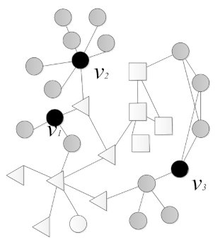
Fueled by the spectacular growth of the internet and Internet of Things, plenty of social networks such as Facebook, Twitter and WeChat have sprung up, changed the mode of interaction between people, and accelerated the development of viral marketing. Originally from the idea of word-of-mouth advertising, viral marketing takes advantage of trust among close social circles of friends, colleagues or families to promote a new product, i.e., when a friend relationship affects a user making decisions on item selection [1,2]. Motivated by applications to early viral marketing, a new study area of influence diffusion has thrived. Therein, the problem of influence maximization is to select a fixed size set of seed nodes in a network to maximize the influence spread according to a specially designed influence diffusion model. Figure 1 gives a toy example of social influence. The nodes $v_1$,$v_2$,$v_3$ in black are the seed nodes which are initially active, and the nodes in gray color are newly activated by the seed nodes. In terms of viral marketing, for example, if user $v_1$,$v_2$,$v_3$ bought a product, their friends in a given social network will likely buy this product because of the friend-to-friend influence.

The applications of influence maximization are prevalent in the real world and include such purposes as viral marketing, anticipating natural hazards, reducing gang violence, public opinion supervision etc., whereas the time complexity of solving the problem of influence maximization is NP hard [3]. This inspires a lot of studies on influence diffusion and influence maximization algorithms. In early time, most studies have focused on the influence maximization algorithms themselves under a general independent cascade (IC) diffusion model or a general linear threshold (LT) diffusion model [4,5], including greedy-based algorithms [3,6,7,8,9,10] and heuristic-based algorithms [11,12,13]. In terms of running time, heuristic-based algorithms are generally more efficient than various greedy-based algorithms, but they do not have any theoretical guarantee.

As in the real world, influence propagation often involves latent variables that are directly unobservable, including influence strength. Estimating influence strength is a fundamental problem for influence diffusion. Some models to estimate influence strength have been proposed, including the topic model [14,15], probabilistic methods [16,17] and models based on deep learning [18,19]. Although existing models and methods have achieved a lot, they demonstrate a number of major drawbacks: (1) conventional approaches propose various humanly devised rules to extract features of user interactions, the effectiveness of which heavily depends on domain expert knowledge. (2) They only consider general network structure and node attributes as factors underlying social network influence, but in the real world, the structure of a large-scale network is more complex and often involves communities, community tensility and node depth in a clustering tree. (3) They are often applicable for special scenarios or specific diffusion models, not for generalized conditions.

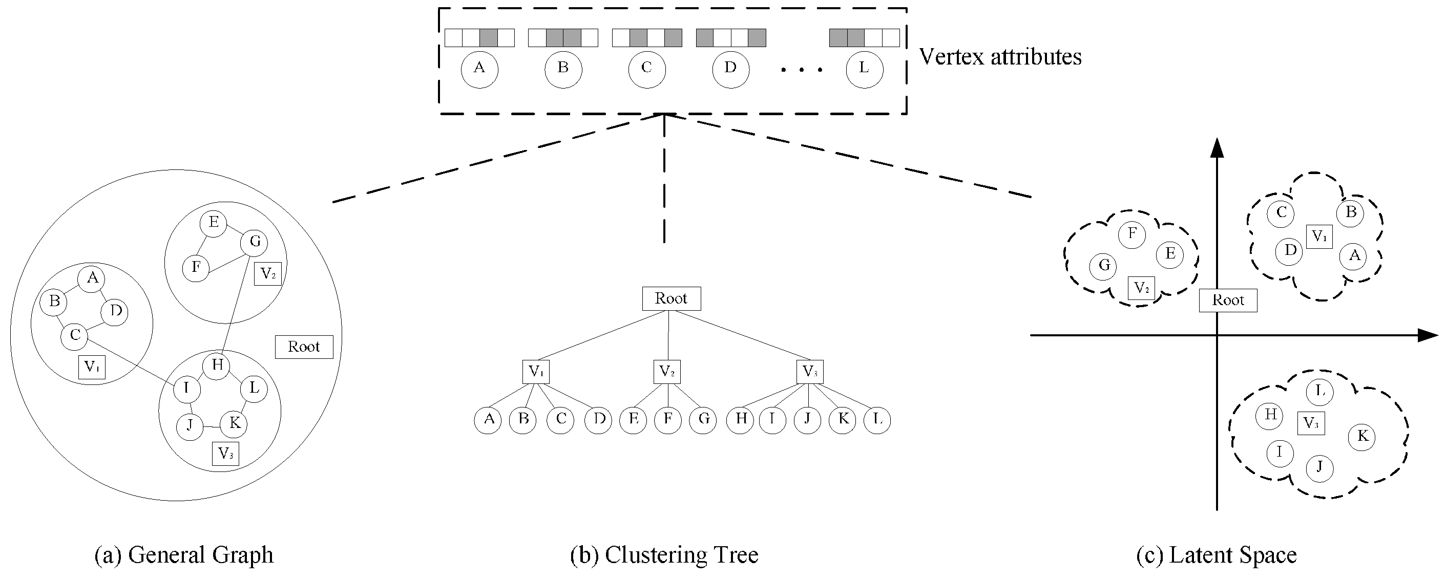
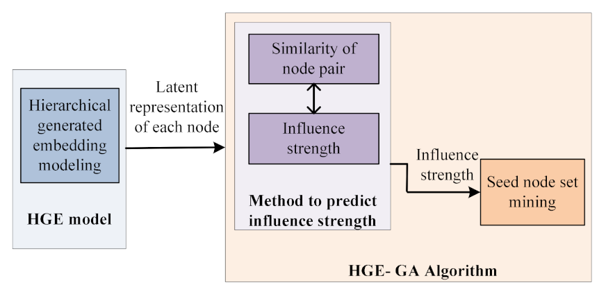
Like most scenarios in real-world propagation [16], influence strength, in this paper, is assumed to be directly unobservable. To predict influence strength, we need to compute the similarity of node pairs, with the motivation originating from previous studies that showed that the more equivalent the network structure and node attributes of two nodes are, the more likely they make similar judgments, even if they have no direct connection reciprocally [20]. Inspired by the powerful ability of neural networks in the field of representation learning, we design a deep hierarchical network embedding model, HGE, to map nodes into latent space automatically, preserving network structures and node attributes as much as possible. The correspondence between the general attributed network and the hierarchical latent space is illustrated in Figure 2. Then, with the learned latent representation of each node, we measure the similarity of node pairs and regard it as the influence probability between two nodes, since the underlying factors of influence probability are network structures and node attributes [20]. Next, the top-K influential nodes can be computed through a greedy-based maximization algorithm. The overview of the proposed method is illustrated in Figure 3.

Social networks usually have millions of users, with a large amount of user-related information, community structures, and complex hierarchical network structures. When embedding nodes into a low-dimensional vector space, in order to preserve network structures as much as possible, hierarchical structures should be taken into account. Furthermore, a community is formed of nodes which have similar attributes while repelling each other due to attribute differences measured by the tensility of the community. In other words, a community is a node set with tensility, and in order to capture this tensility, we embed a community as a Gaussian distribution. Specifically, we propose a hierarchical generative embedding model which integrates hierarchical community structure, node attributes and general network structure into a unified generative framework.

To summarize, we make the following contributions:

(1) We study the problem of incorporating hierarchical generative embedding into influence strength prediction for the first time;

(2) In order to predict influence strength, we propose a novel model, the HGE model, which automatically maps nodes into latent space, avoiding humanly devising rules to extract features of user interactions. The proposed HGE model integrates hierarchical community structure, node attributes and general network structure into a unified generative framework that ensures the preservation of node characteristics and captures the granularity of hierarchical characteristics as well as community tensility in an attributed network effectively. Furthermore, we propose a new algorithm, HGE-GA, to predict influence strength and compute the top-K influential nodes effectively. The proposed HGE-GA algorithm can be generalized to different scenarios or diffusion models;

(3) We evaluate our method on various datasets and tasks, and experimental results show that the proposed model and algorithm significantly outperform the state-of-the-art approaches.

The rest of this paper is organized as follows. Section 2 reviews related work. Section 3 presents notations and problem formulation. Section 4 details the proposed method. Section 5 lists the experiment setup. Section 6 presents the experimental results & analysis. Section 7 concludes the paper.

2. Related Work

Influence Diffusion. The studies of influence diffusion focus on the key factors for influence diffusion, such as diffusion models of a single entity or multiple entities, as well as the influence probability between two nodes, which is more relevant to our work. Estimating influence probability between two nodes (or influence strength) is a fundamental problem for influence diffusion, since in real-world propagation scenarios, the variables such as influence strength and infection time may be not directly observed. Some models to estimate influence strength have been proposed. One line of research is based on topic extraction and lays emphasis on incorporating the topic model into influence diffusion. Ref. [15] proposes a latent variable model, which captures community-level topic interest, item-topic relevance and community membership distribution of each user and further infers user-to-user influence strength. Ref. [14] proposes a novel model, COLD, to model community-level influence diffusion. Another line of studies utilize various probabilistic methods such as Bayesian inference [16] and EM (Expectation maximization) [17] to stimulate influence diffusion and learn the parameters in the generative model. Recently, researchers have endeavored to build models of influence prediction using deep learning, which can predict social influence automatically and are no longer limited to expert knowledge when extracting user features or network features. Ref. [18] proposes a recurrent neural variational model (RNV) to dynamically track entity correlations and cascade correlations. Ref. [19] proposes the DeepInf model to predict social influence, which detects the dynamics of social influence and integrates network embedding and graph attention mechanisms into the model. Ref. [21] proposes a reinforcement learning framework to discover effective network sampling heuristics by leveraging automatically learned node and graph representations.

To the best of our knowledge, the existing models to predict the influence probability between two nodes usually extracts features of user interactions with various humanly devised rules, which heavily depends on expert knowledge of this domain. Besides, the underlying factors that affect social network influence, such as communities, community tensility and node depth in a clustering tree, have not been taken into account in the existing models when computing the influence probability of node pairs. Moreover, the existing models are often applicable for special scenarios or specific diffusion models, not for generalized conditions.

Network Embedding. Network embedding techniques aim at inferring representations, also called embeddings, of entities in the networks. The basic idea of network embedding is to embed the nodes into a low-dimensional vector space in which the similarity between nodes can be measured and network structures can be preserved as much as possible. Many downstream learning tasks can benefit from this form of representation, such as link prediction, node classification, node clustering and network visualization.

Existing models of network embedding are concerned about the technology of mapping or dimension reduction. In order to obtain effective low-dimensional embeddings, numerous algorithms have been proposed. Inspired by Word2Vec [22], deep learning has been migrated to network embedding. DeepWalk [23], Node2Vec [24] and Line [25] extract a number of sequential nodes in the network by random walk. Nodes in a sequence are metaphorically equivalent to words in language models. Skip-Gram [22] is then employed to obtain the embeddings of nodes. After obtaining the embeddings of nodes, the similarity of nodes can be calculated by the inner-product of their embeddings. LINE [25] uses first-order and second-order proximities and trains the model via negative sampling. SDNE [26] adopts a deep auto-encoder to preserve both the first-order and second-order proximities.

As one of the most important features of social networks, community structure is usually integrated into network embedding as auxiliary information [27,28,29,30]. M-NMF [27] incorporates the community structure into network embedding and exploits the consensus relationship between the representations of nodes and community structure. M-NME then jointly optimize NMF (Network Matrix Factorization)-based representation learning model and modularity-based community detection model in a unified framework. GraphAGM [28] combines AGM [31] and GAN [30] in a unified framework which can generate the most likely motifs with graph structure awareness in a computationally efficient way. NECS [29] preserves the high-order vertex proximity and incorporates the community structure of networks in vertex representation learning.

Hierarchical Network Embedding. The community structures in complex networks are often hierarchical [32,33,34,35,36]. Inspired by the natural hierarchical structure of a galaxy with its stars, planets, and satellites, ref. [33] proposes the galaxy network embedding (GEM) model. GEM captures hierarchical structures by forming an optimization problem, including pairwise proximity, horizontal relationships and vertical relationships. In order to solve various defects caused by the exponential decay of the radius in the GEM model, Long et al. [36] first apply subspace to hierarchical network embedding and propose the SpaceNE model, which preserves proximity between pairwise nodes and between communities. Ref. [35] proposes NetHiex, a network embedding algorithm which can capture the different levels of granularity and alleviate data scarcity. Ma et al. [37] propose the MINES framework, which can embed multi-dimensional networks with a hierarchical structure to low-dimensional vector spaces, with the learned representations for each dimension containing the hierarchical information. Nickel et al. [38] use hyperbolic space instead of Euclidean space to capture hierarchical structures in networks. The learned embeddings are difficult to convert into Euclidean space, which is inappropriate for some downstream tasks of machine learning.

However, these hierarchical embedding algorithms suffer from some defects: (1) They embed each node or community as a vector in the latent space, which ignores the tensility of the community. Essentially, a community is a set of nodes or smaller communities with similar attributes and tensility, and a simple vector can not represent this relationship of affiliation. The tensility of a community has been defined in Definition 2. (2) They do not consider node depth in a clustering tree when dealing with vertical relationships in a hierarchical network. Thus, it is inappropriate to use the traditional method of measuring vertical relationships in a hierarchical network to compute vector distance in latent space. The granularity of hierarchical structures should be taken into account, and a personalized method to measure vector distance in latent space should be designed. The granularity of hierarchical structures has been defined in Definition 3.

3. Notations and Problem Formulation

In this section, we first introduce the definitions and notations, and then formulate the problem studied in this paper.

Definition 1 (attributed network). 

An attributed network is an undirected graph $\mathcal{G} = (\mathcal{V},\mathcal{E},\mathcal{A})$, where $\mathcal{V}$ is the set of network nodes, $\mathcal{E}$ is the set of edges and $\mathcal{A}\in {\{0,1\}}^{\left|\mathcal{V}\right| \times F}$ is a binary-valued attribute matrix recording node-attribute associations, with F being the number of attributes. The element $A_{i,a}\in \mathcal{A}$ is a binary-valued attribute weight, indicating that attribute a associates with node i if $A_{i,a} = 1$.

Definition 2 (the tensility of community). 

A community is a set composed of nodes with similar attributes. These nodes form a community due to similar attributes and repel each other in the community due to differences in attributes. The tensility of the community is used to measure the difference of node attributes in the community.

Definition 3 (the granularity of hierarchical characteristics). 

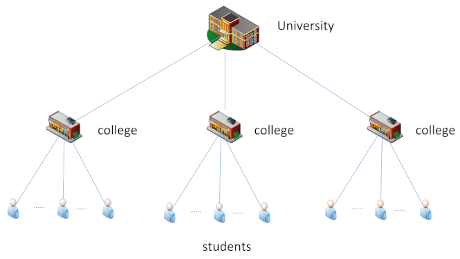
In hierarchical networks, vertexes at different levels have different granularities of characteristics. As shown in Figure 4, the university in the top level has the characteristics of name, address etc., and the colleges in the second level have the characteristics of majors, number of students etc. The characteristics of nodes at different levels have different granularities, while the granularity of the characteristics is the same for the nodes at the same level. It is the granularity of hierarchical characteristics that causes the vertical constraint of hierarchical structure properties (see Section 4.1.1).

The hierarchical clustering tree of G is denoted as T with a depth of L. ${\mathcal{V}}^l$ is the vertex set at the l-th level of T, and $v_i^l\in {\mathcal{V}}^l$ is the i-th vertex at the l-th level. $Ch(v)$ denotes the child vertex set of the vertex v, $fa(v)$ denotes the father vertex of v and $\mathsf{\Phi }(v)$ denotes the embedding of vertex v. In our paper, we use ’vertex’ to represent a user or community in the hierarchical network, while using ’node’ to represent a user in the general network, especially when $l = L$, $v_i^l$ represents a leaf vertex (user) at the bottom of the clustering tree. For ease of reference, we summarize the basic notations in

Table 1. Main notation used across the whole paper.

Notation	Description
$\mathcal{G}$	An undirected graph
$\mathcal{V}$	Set of nodes
$\mathcal{E}$	Set of edges
T	A hierarchical clustering tree
L	The depth of the clustering tree
$\mathcal{C}h(v)$	The child vertex set of vertex v
$fa(v)$	The father vertex of v
$v_i^l$	The i-th vertex at the l-th level
${\mathsf{\Phi }}_v$	The embedding of vertex v

.

With the definitions and notations described above, we formulate the problem studied.

Problem 1 (Node Embedding). 

Given an undirected graph $\mathcal{G} = (\mathcal{V},\mathcal{E},\mathcal{A})$, the goal is to learn the latent representation of nodes with the mapping function Ξ:

$$\mathcal{G}\stackrel{\Xi }{⟶}{\mathsf{\Phi }}_{\mathcal{V}}$$

(1)

such that the information of hierarchical network structure, general network and node attributes can be preserved as much as possible by ${\mathsf{\Phi }}_{\mathcal{V}}\in {\mathcal{R}}^{N \times D}$, where ${\mathsf{\Phi }}_{\mathcal{V}}$ is the latent embedding matrix for all nodes and D is the dimension size of the embeddings.

Problem 2 (Influence Maximization in Attributed Social Networks). 

Given an IC diffusion model, an undirected graph $\mathcal{G} = (\mathcal{V},\mathcal{E},\mathcal{A})$ and the latent embedding matrix for all nodes ${\mathsf{\Phi }}_{\mathcal{V}}$, the goal is to find the node set $\mathcal{S}$ with an algorithm $\mathcal{F}$:

$$\mathcal{G},{\mathsf{\Phi }}_{\mathcal{V}}\stackrel{\mathcal{F}}{⟶}\mathcal{S}$$

(2)

such that the expected spread of node set $\mathcal{S}$, i.e., $\sigma (\mathcal{S})$, is maximized and $\left|\mathcal{S}\right| = K$. The expected spread of node set $\mathcal{S}$ is defined as the total number of active nodes after the influence spread ends, including the newly activated nodes and the initially active nodes.

4. The Proposed Method

Like most scenarios in real-world propagation [16], the influence probability of node pairs, in this paper, is assumed to be directly unobservable. To predict the influence probability of node pairs, we first embed the nodes into a low-dimensional vector space by jointly modeling the horizontal constraint, vertical constraint, affiliation constraint and node attributes. After obtaining the embedding of each node, we use the two-normal form to measure the similarity of the node pair. Then we predict the influence probability of the node pair with the measured similarity of the node pair. We now describe the proposed method in the following subsections: the hierarchical generative embedding model is described in Section 4.1, the learning procedure is described in Section 4.2, and the HGE-GA algorithm is described in Section 4.3.

4.1. Hierarchical Generative Embedding Model

The proposed HGE model focuses on preserving the following characteristics of the network: (1) Horizontal structure characteristics. Nodes belonging to the same community are more similar than nodes belonging to different communities (in terms of blood relations, blood brothers are closer than cousins). (2) Vertical structure characteristics. The more children a node has, the more genes it inherits from its father; that is, the more similar it is to its father. (3) Affiliation relationship characteristics. Users in the same community often have both similarities and differences between them. Differences between nodes are defined as the tensility of node and should be preserved. (4) General network structure characteristics. In a general network, the more similar the nodes are, the closer they are in the embedding space. (5) Node attribute characteristics. Node attributes provide rich information regarding node characteristics, which should be taken advantage of for preserving node characteristics in latent space.

We will detail the HGE model from three aspects. The first one is how to preserve the hierarchical network structure, the second one is how to capture general network structure properties, and the third one is how to acquire node attribute features.

4.1.1. Hierarchical Structure Properties

Similar to most embedding methods [23,24,25], we preserve the network structure through the distance of the vertex in the hidden space. A community is a node set with tensility, and in order to capture this tensility, we embed a community as a Gaussian distribution. The greater the variance, the greater tensility of the community, that is, the difference between nodes contained in the community will be greater. Therefore, we use the KL distance to measure the similarity between communities. More specifically, suppose ${\mathsf{\Phi }}_{v_1} = \mathcal{N}({\mu }_1,{\mathsf{\Sigma }}_1)$, ${\mathsf{\Phi }}_{v_2} = \mathcal{N}({\mu }_2,{\mathsf{\Sigma }}_2)$. Then, the distance between $v_1$ and $v_2$ can be calculated in two ways, as follows:

$$\begin{array}{cc}\hfill & \delta (v_1,v_2) = D_{KL}({\mathcal{N}}_1\parallel {\mathcal{N}}_2) = \frac{1}{2}[tr({\mathsf{\Sigma }}_2^{-1}{\mathsf{\Sigma }}_1)\hfill \\ \hfill & + {({\mu }_2 - {\mu }_1)}^T{\mathsf{\Sigma }}_2^{-1}({\mu }_2 - {\mu }_1) - L - log\frac{{\mathsf{\Sigma }}_2}{{\mathsf{\Sigma }}_1}].\hfill \end{array}$$

(3)

where $tr({\mathsf{\Sigma }}_2^{ - 1}{\mathsf{\Sigma }}_1)$ is the trace of matrix ${\mathsf{\Sigma }}_2^{ - 1}{\mathsf{\Sigma }}_1$, $v_1$ and $v_2$ are communities, and L is a constant.

$$\begin{array}{c}\hfill \delta (v_1,v_2) = {∥{\mu }_1 - {\mu }_2∥}_2\end{array}$$

(4)

where $v_1$ and $v_2$ are nodes.

Unlike normal networks, hierarchical networks contain a large number of hierarchical relationships. To capture this complex hierarchical relationship, we force the embedding of a vertex to submit to two constraints, the horizontal and the vertical:

Horizontal constraint: Generally, community-based embedding methods [27,28] consider that the nodes belonging to the same community are more similar than those belonging to different communities. Thus, we intend to extend this constraint to hierarchical networks and name such a constraint as the horizontal constraint. The horizontal constraint can be defined as follows: For each layer l in clustering tree T, for all vertex-pairs $v_i^l$, $v_j^l$ at layer l with $fa(v_i^l) = fa(v_j^l)$, for all $v_k^l$ at layer l with $fa(v_i^l)\ne fa(v_k^l)$ and $fa(v_j^l)\ne fa(v_k^l)$, we have

$$\begin{array}{c}\hfill \delta (v_i^l,v_j^l) < \delta (v_i^l,v_k^l)\end{array}$$

(5)

$$\begin{array}{c}\hfill \delta (v_i^l,v_j^l) < \delta (v_j^l,v_k^l)\end{array}$$

(6)

Vertical constraint: From the biological point of view, a clustering tree can be likened to a gene tree, in which the lower vertexes propagate from the upper vertexes. The more children a vertex has, the more genes it inherits from its father, that is, the more similar it is to its father. We use a personalized distance rank method to describe the vertical constraint: for all vertices m,

$$\begin{array}{c}\hfill \delta (v_1,v_m) < \delta (v_2,v_m) < \cdots < \delta (v_n,v_m)\end{array}$$

(7)

if $n(v_1) > n(v_2)\cdots > n(v_n)$, where $v_1,v_2,\cdots ,v_n$ are children of $v_m$, i.e., $v_1,v_2,\cdots ,v_n\in \mathcal{C}h(v_m)$, and $n(v_1),n(v_2),\cdots ,n(v_n)$, respectively, denote the number of the children of vertices $v_1,v_2\cdots v_n$.

Affiliation constraint: In hierarchical networks, bottom-node clustering forms small communities, while small-community clustering forms large communities. Therefore, the parent node can be regarded as the feature set of all child nodes. Our HGE model describes the formation process of hierarchical networks from the perspective of generation: as the attribute set of the entire hierarchical network, the root node generates the child node of the next layer according to the attribute classification and repeats this top-down generation process to obtain the entire hierarchical network. In order to capture this hierarchical affiliation (generation) relationship, in the HGE model, nodes are embedded as Gaussian distributions. The mean value represents the position in the embedding space and is generated by the distribution of the parent node, and the variance represents the tensility of the node, which can also represent the differences among all child nodes. In particular, the leaf node has no tensility; that is, the variance of the embedding is 0.

A community is a small group of users who have the same hobbies, occupations, social relations and so on. Users in the same community often have similar attributes. Traditional community-based embedding methods always focus on how to capture the similarity between nodes in the same community [27], which ignores the differences between nodes. The affiliation constraint can be defined as follows: for vertex $v_i^l$ and his father vertex $v_j^{l - 1}$, ${\mathsf{\Phi }}_i^l = \mathcal{N}({\mu }_i,{\mathsf{\Sigma }}_i)$, ${\mathsf{\Phi }}_j^{l - 1}=\mathcal{N}({\mu }_j,{\mathsf{\Sigma }}_j)$, where the ${\mu }_i$ is sampled from the hyper-distribution ${\mathsf{\Phi }}_j^{l - 1}$, i.e.,  ${\mu }_i\sim \mathcal{N}({\mu }_j,{\mathsf{\Sigma }}_j)$. In particular, when $i = T$ (vertex i is at the bottom layer), ${\mathsf{\Phi }}_i^l = \mathcal{N}({\mu }_i,0)$.

4.1.2. General Network Structure Properties

In order to preserve the structure of the general network, we keep the embedding of nodes to satisfy the first-order proximity and the second-order proximity. The first-order proximity posits that, for each pair of nodes $v_1$ and $v_2$ linked by an edge($v_1$, $v_2$), the similarity between $v_1$ and $v_2$ should be greater than that of two nodes without an edge connection, and the second-order proximity keeps each node pair($v_1$, $v_2$) that share the same neighborhood similar.

4.1.3. Node Attribute Properties

Given a node i with an attribute a, the logistic model is used with a mean value of the multidimensional Gaussian distribution of node i, i.e., ${\mu }_i$, as input features to predict the probability of node i associating with attribute a:

$$\begin{array}{c}\hfill R_{i,a} = \sigma (W_a^T{\mu }_i + b),\end{array}$$

(8)

where $W_a$ is the logistic weight factor, b is the bias and $\sigma (.)$ is a logistic function defined as $\sigma (x) = {(1+e^{-x})}^{-1}$.

4.2. Learning Procedure

In this subsection, we will introduce the learning procedure of the HGE model. Like most unsupervised embedding models, we formulate network structure preservation as an optimization problem. By optimizing the lower bound of the corresponding loss function, the HGE model converges. Our loss function can be divided into three independent parts, corresponding to the capture of the structure of the hierarchical network, general network and node attributes.

4.2.1. Hierarchical Network Optimization

First, the similarity of the same community node is captured by optimizing the lower bound of the loss function. Nodes in the same community can be closer in the hidden space, while nodes in different communities will be pushed farther apart. This can be defined as follows:

$$\begin{array}{c}\hfill {\mathcal{L}}_{hor} = \sum _{l = 3}^T\sum _{\begin{array}{c}i,j,k\in {\mathcal{S}}_l,\\ fa(v_i^l) = fa(v_j^l)\ne fa(v_k^l)\end{array}}\delta {(v_i^l,v_j^l)}^2 + ex{p}^{-\delta (v_i^l,v_k^l)},\end{array}$$

(9)

where ${\mathcal{S}}_l$ is the vertex set of layer l, and T is the depth of the clustering tree.

In order to capture the hierarchical vertical relationship, we use the following loss function to achieve the personalized distance ranking in Equation (7), as shown below:

$$\begin{array}{c}\hfill {\mathcal{L}}_{ver} = \sum _{l=1}^{T - 1}\sum _{\begin{array}{c}i,j\in {\mathcal{S}}_l,\\ fa(v_i^l) = fa(v_j^l)\end{array}}\delta {(v_i^l,fa(v_i^l))}^2 - ex{p}^{\delta (v_j^l,fa(v_i^l))},\end{array}$$

(10)

when $n(v_i^l) < n(v_j^l)$.

To capture hierarchical affiliation, the HGE model assumes that the mean of the node embedding is subordinated to the Gaussian distribution corresponding to its father vertex. We use maximum likelihood to approximate the embedding of the father node. For an arbitrary vertex i, suppose that vertices $v_1$, $v_2$, …, $v_m$ are children of vertex i with ${\mathsf{\Phi }}_{v_1} = \mathcal{N}({\mu }_1,{\mathsf{\Sigma }}_1)$, ${\mathsf{\Phi }}_{v_i} = \mathcal{N}({\mu }_i,{\mathsf{\Sigma }}_i)$, …, ${\mathsf{\Phi }}_{v_m} = \mathcal{N}({\mu }_m,{\mathsf{\Sigma }}_m)$. Then, the maximum likelihood function can be defined as follows:

$$\begin{array}{c}L(\mu ,\mathsf{\Sigma }) = \prod _{i = 1}^{m}f({\mu }_i;\mu ,\mathsf{\Sigma })\hfill \\ \hspace{1em}\hspace{1em}=\prod _{i = 1}^m{(2\pi )}^{-\frac{n}{2}}{\left|\mathsf{\Sigma }\right|}^{-\frac{1}{2}}exp(-\frac{1}{2}{({\mu }_i - \mu )}^T{\mathsf{\Sigma }}^{-1}({\mu }_i - \mu ))\\ \hfill \hspace{1em}\hspace{1em}\hspace{1em}\hspace{1em}\hspace{1em}\hspace{1em}\hspace{1em}\hspace{1em}\hspace{1em}\hspace{1em}\hspace{1em}\hspace{1em}\hspace{1em}\hspace{1em}\hspace{1em}\hspace{1em}\hspace{1em}={(2\pi )}^{ - \frac{mn}{2}}{\left|\mathsf{\Sigma }\right|}^{-\frac{m}{2}}exp(-\frac{1}{2}\sum _{i = 1}^m{({\mu }_i-\mu )}^T{\mathsf{\Sigma }}^{-1}({\mu }_i-\mu ))\end{array}$$

(11)

where n is the dimension of $\mu$.

The logarithmic likelihood function is:

$$\begin{array}{c}lnL(\mu ,\mathsf{\Sigma }) = ln{(2\pi )}^{-\frac{mn}{2}}+ln{\left|\mathsf{\Sigma }\right|}^{-\frac{m}{2}}\hfill \\ \hspace{1em}\hspace{1em}+lnexp(-\frac{1}{2}\sum _{i = 1}^m{({\mu }_i-\mu )}^T{\mathsf{\Sigma }}^{-1}({\mu }_i - \mu ))\\ \hfill \hspace{1em}\hspace{1em}\hspace{1em}\hspace{1em}\hspace{1em}\hspace{1em}\hspace{1em}\hspace{1em}\hspace{1em}\hspace{1em}\hspace{1em}\hspace{1em}\hspace{1em}\hspace{1em}\hspace{1em}\hspace{1em}\hspace{1em}\hspace{1em}\hspace{1em}\hspace{1em}= C -\frac{m}{2}ln\left|\mathsf{\Sigma }\right|-\frac{1}{2}\sum _{i = 1}^m{({\mu }_i - \mu )}^T{\mathsf{\Sigma }}^{-1}({\mu }_i - \mu )),\end{array}$$

(12)

where C is a constant.

We use the negative logarithmic maximum likelihood as the loss function to capture hierarchical affiliation:

$$\begin{array}{c}\hfill {\mathcal{L}}_{aff} = -lnL(\mu ,\mathsf{\Sigma })\end{array}$$

(13)

To sum up, the objective function to capture the hierarchical network structure can be defined as follows:

$$\begin{array}{c}\hfill {\mathcal{L}}_{hie} = {\mathcal{L}}_{hor} + {\mathcal{L}}_{ver} + {\lambda }_1{\mathcal{L}}_{aff},\end{array}$$

(14)

where ${\lambda }_1$ is a trade-off parameter to balance the three parts of the loss function ${\mathcal{L}}_{hierarchical}$. We can optimize the parameters such that the loss ${\mathcal{L}}_{hierarchical}$ is minimized; thus, the three constraints we proposed can be satisfied.

4.2.2. General Network Optimization

Following the LINE model [25], we construct our unsupervised training loss based on the first-order and second-order proximities, which is an efficient unsupervised learning objective for graph data and can capture both the direct and indirect similarities between nodes in a general network.

$$\begin{array}{c}\hfill {\mathcal{L}}_1 = -\sum _{(v_i,v_j)\in \mathcal{E}}{w}_{i,j}log{p}_1(v_i,v_j)\end{array}$$

(15)

$$\begin{array}{c}\hfill {\mathcal{L}}_2 = -\sum _{(v_i,v_j)\in \mathcal{E}}{w}_{i,j}log{p}_2(v_j|v_i)\end{array}$$

(16)

$$\begin{array}{c}\hfill {\mathcal{L}}_{ns} = {\mathcal{L}}_1 + {\mathcal{L}}_2\end{array}$$

(17)

where the ${\mathcal{L}}_1$ and ${\mathcal{L}}_2$ are the first-order and second-order objectives, and Ons is the node similarity objectives of our model. The probability $p_1$ and $p_2$ are computed as:

$$\begin{array}{c}\hfill p_1(v_i,v_j) = \frac{1}{1 + exp(-{({\mu }_i)}^T · {\mu }_j)},\end{array}$$

(18)

$$\begin{array}{c}\hfill p_2(v_j|v_i) = \frac{exp({({\mu }_j)}^T · {\mu }_i)}{{\sum }_{k = 1}^{V}exp({({\mu }_k)}^T · {\mu }_i)},\end{array}$$

(19)

The ${\mathcal{L}}_2$ can further be optimized by the negative sampling.

4.2.3. Node Attribute Optimization

Incorporating Equation (8), the loss function of this part is defined as follows:

$$\begin{array}{c}\hfill {\mathcal{L}}_A = D_{KL}(\widehat{R}\Vert R) = -\sum _{i\in \mathcal{V}}\sum _{A_{i,a}\in \mathcal{A}}{A}_{i,a}log{R}_{i,a},\end{array}$$

(20)

where $A_{i,a}\in \mathcal{A}$ is a binary-valued attribute weight indicating that attribute a associates with node i if $A_{i,a} = 1$, $\widehat{R}$ is the empirical distribution of the attribute weight with the empirical distribution of node i associating with attribute a, i.e., ${\widehat{R}}_{i,a}$, being simply set as $A_{i,a}$. Note that all the attributes in this paper are binary-valued. Although ${\widehat{R}}_{i,a}$ is applicable for not only binary-valued attributes but also real-valued attributes, we focus primarily on binary-valued attributes in this paper.

To summarize, the final objective ${\mathcal{L}}_{final}$ of our model can be written by the sum of the ${\mathcal{L}}_{hie}$, ${\mathcal{L}}_{ns}$ and ${\mathcal{L}}_A$:

$$\begin{array}{c}\hfill {\mathcal{L}}_{final} = {\mathcal{L}}_{hie} + {\mathcal{L}}_{ns} + {\mathcal{L}}_A,\end{array}$$

(21)

in which the ${\mathcal{L}}_{final}$ can be optimized by the Adam method.

To ensure that embedding can preserve both vertical and horizontal features after training, the whole embedding process is executed from the bottom up. For each node $v_i^l$ at layer l, the learned representation can be obtained after optimizing the horizontal loss of layer l and the vertical loss at layer $i + 1$ with Adam.

4.3. HGE-GA Algorithm

It has been proposed by previous work on social network influence [20] that the more equivalent the network structure of two nodes is, the more likely they make similar judgments, even without an edge between them, because these two nodes connect to other nodes more identically. It has also been revealed by previous studies on social networks that the opinions and behaviors of nodes are affected by node attributes [20], i.e., similar attributes of nodes cause similar behaviors. Therefore, the similarity of network structures and node attributes are the two factors underlying the influence probability between two nodes. We measure the similarity of node pairs and predict the influence probability of node pairs with the embedding of nodes inferred from the proposed HGE model. With the predicted influence probability of node pairs, we utilize a general greedy strategy to compute the top-K influential nodes in the network. The proposed HGE-GA algorithm is outlined in Algorithm 1, and will be detailed in this subsection.

Algorithm 1: HGE-GA Algorithm

Input: social network $\mathcal{G}=(\mathcal{V},\mathcal{E},\mathcal{A})$, the embeddings of all nodes $\mathsf{\Phi }$, seed set size K. Output: Seed node set $\mathcal{S}$. 1:  predicts influence probability of arbitrary pairwise nodes, $p_{u,v}$; 2:  for$j = 1\dots K$do 3:     $u^{*}\leftarrow arg{max}_{u^{*}\in \mathcal{U}}\sigma (\mathcal{S}\cup u^{*}) - \sigma (\mathcal{S})$; 4:     $\mathcal{S} = \mathcal{S}\cup u^{*}$; 5:  end for 6:  return$\mathcal{S}$;

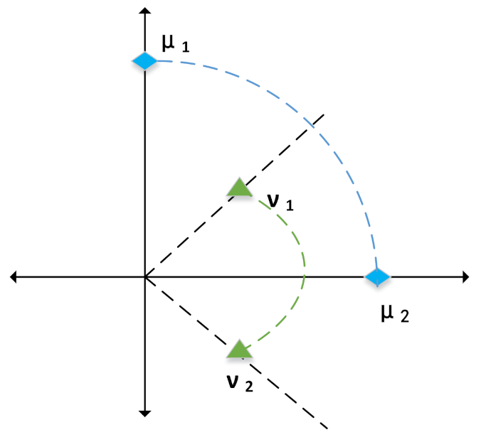
Traditional network representation methods embed nodes into a low-dimensional vector space, and they always use the inner product to measure the similarities of node pairs. Then the relationships between node pairs can be captured. However, this method cannot capture the relationships among neighborhoods of nodes in some cases. As shown in Figure 5, for a node $v_1$ and its two neighborhoods $u_1$ and $u_2$, two relationships are represented, as follows:

$$\begin{array}{cc}\hfill & v_1 · u_1 = v_1 · u_2,\hfill \\ \hfill & u_1 · u_2 = 0\hfill \end{array}$$

(22)

As neighbors of node $v_1$, nodes $u_1$ and $u_2$ are similar in attributes, but the method based on the inner product cannot capture the relationship between $u_1$ and $u_2$ in the latent space. Similarly, the relationship between node $v_1$ and $v_2$ can not be captured by using the inner product.

To avoid the case shown in Equation (26), we use the two-normal form, which satisfies the critical triangle inequality. The norm of a vector can simply be understood as its length or the corresponding distance between two points. The two-normal form is a common way to measure distance between vectors. Using the two-normal form, we define the relationship between node i and node j as follows:

$$g({\mathsf{\Phi }}_i,{\mathsf{\Phi }}_j)={∥{\mathsf{\Phi }}_i - {\mathsf{\Phi }}_j∥}_2$$

(23)

The above relationship with the two-normal form adequately captures the similarity of two nodes. We regard the similarity of two nodes as the influence probability between two nodes, since the similarity of the network structure and node attributes are the two factors underlying the influence probability between two nodes. Thus, the influence probability between node i and j, i.e., $p_{i,j}$ can be predicted as follows.

$$p_{i,j} = g({\mathsf{\Phi }}_i,{\mathsf{\Phi }}_j) = {∥{\mathsf{\Phi }}_i - {\mathsf{\Phi }}_j∥}_2$$

(24)

After obtaining the influence probability of arbitrary pairwise nodes, under a general independent cascade (IC) diffusion model, we utilize a general greedy strategy to compute the top-K influential nodes, as Algorithm 1 shows.

5. Experiment Setup

We quantitatively evaluate the performance of the proposed HGE model in downstream learning tasks (vertex classification, link prediction, network visualization) and compare the proposed algorithm, HGE-GA, with the state-of-art influence maximization algorithms using the metric of expected spread on several large-scale real-world datasets. In this section, we will detail the experimental setup, including research questions (Section 5.1), datasets (Section 5.2), baselines (Section 5.3), evaluation metrics and experimental settings (Section 5.4).

5.1. Research Questions

We aim at answering the following research questions to evaluate the performance of the proposed HGE model and HGE-GA algorithm.

(RQ1) How does the proposed HGE model perform in terms of traditional graph-mining tasks, e.g., vertex classification, link prediction and network visualization, compared with baselines?

(RQ2) Can the proposed influence maximization algorithm, HGE-GA, outperform the state-of-art influence maximization algorithms with respect to the expected spread?

(RQ3) Does the two-normal form to measure distance contribute to the improvement of the performance of the proposed algorithm?

5.2. Datasets

We use four datasets, the detailed properties of which are shown in

Table 2. Statistics of the datasets used in the experiments.

	#Nodes	#Edges	#Attributes	#Labels
Cora	2708	5429	1433	7
DBLP	17,716	105,734	1639	4
BlogCatalog	5196	171,743	8189	6
Flickr	7575	239,738	12,047	9
Pubmed	19,717	44,338	500	3

.

• Cora [39]: The Cora dataset is a citation networks which is composed of a large number of academic articles. Nodes are publications and edges are citation links;
• DBLP: The DBLP dataset consists of bibliography data in computer science. Each paper may cite or be cited by other papers, which naturally forms a citation network;
• BlogCatalog: This dataset is a social relationship network which is crawled from the BlogCatalog website. BlogCatalog is composed of bloggers and their social relationships. The labels of nodes indicate the interests of the bloggers;
• Flickr: Flickr is a social network where users can share pictures and videos. In this dataset, each node is a user, and each side is a friend relationship between users. In addition, each node has a label that identifies the user’s interest group;
• Pubmed: Pubmed is a public search database that provides biomedical paper and abstract search services. In this dataset, nodes are publications and edges are citation links;

5.3. Baselines

We evaluated the performance of the proposed HGE model compared with the following baselines:

• GraphSAGE [40]: an attributed network embedding model which leverages node attributes and generates embeddings by sampling and aggregating features from a node’s local neighborhood;
• AANE [41]: a model which learns attributed network embedding efficiently by decomposing complex modeling and optimization into sub-problems;
• M-NMF [27]: a single-layer community structure preserving baseline, which integrates the community information through a matrix factorization;
• GNE [33]: a multi-layer community structure preserving baseline, which embeds communities onto surfaces of spheres;
• SpaceNE [36]: a method which applies subspace to the hierarchical network embedding model and preserves the proximity between pairwise nodes and between communities;

Moreover, we evaluate the performance of the proposed HGE-GA algorithm compared with the following baselines:

• PMIA [12]: This is a heuristic algorithm that defines the maximum influence in-arborescence (MIIA) and leverages sequence submodularity to compute the influence spread;
• IMM [9]: This utilizes a classical statistical tool, martingale, as well as RR sets (reverse reachable sets), and can provide higher efficiency in practice;
• TSH-GA: Zhou et al. [20] propose a method to compute the influence probability of node pairs, which considers social ties, general network structure, and node attributes as factors underlying influence but executes feature extraction of these three factors by typically hand-crafted rules. TSH-GA is an influence maximization algorithm jointing the method to compute the influence probability of node pairs proposed in [20] and the general greedy algorithm;
• HGE-1N-GA: This is a variant of our HGE-GA which uses the one-normal form to compute the similarity of two nodes.

5.4. Evaluation Metrics and Experimental Settings

Evaluation metrics for the proposed HGE model. We evaluate the performance of link prediction of HGE in terms of the area under the curve (AUC) and average precision (AP). We evaluate the performance of vertex classification in terms of the F1-measure (F1), which is defined as $F1 = \frac{2 · Precision · Recall}{Precision + Recall}$.

Evaluation metric for the proposed HGE-GA algorithm. We evaluate the overall performance of our HGE-GA algorithm by adopting the expected spread as the evaluation metric. This is an extensively used metric for the influence maximization problem. The expected spread is defined as the expected number of active nodes in the network, including the newly activated nodes and the set of seed nodes that were initially active (seed node set) after the influence spread is over (there are no more nodes being activated), given the seed set size K, which is an integer.

Experimental settings. All embedding sizes are 64, and the number of training epochs is 1000. The initial learning rate of Adam is set as 0.001. All results are obtained by averaging 10 experiments. We implement all the baselines by the codes released by the authors. The parameters of the baselines are tuned to be optimal or set according to the corresponding literature. All algorithms are run under the IC diffusion model. Furthermore, for the two algorithms PMIA and IMM, which do not have the step of predicting influence probability of node pairs, we set the propagation probability from node u to node v, i.e., $p(u,v)$, as $1/i$, where i denotes the number of incoming edges of node v. This method of setting influence probability is extensively adopted in previous literature [12].

6. Results and Analysis

6.1. Performance of Vertex Classification of HGE Model

Vertex classification is one of the most important tasks to detect the performance of embedding models. In this section, we perform vertex classification task to evaluate the performance of the learned embeddings and compare with the baseline methods. We choose three datasets (DBLP, BlogCatalog and Flickr) which have ground-truth classes. To be specific, we first sample a small number of nodes as training data, and the rest is used as test data. Similar to [23], we use one-vs-rest logistic regression for node classification, and the training data size is $10\%$; the results are reported in

Table 3. Node classification performance.

Method	DBLP	BlogCatalog	Flickr
	F1	F1	F1
AANE	0.702	0.515	0.517
GraphSAGE	0.731	0.625	0.649
M-NMF	0.524	0.604	0.587
GNE	0.741	0.623	0.631
SpaceNE	0.767	0.654	0.651
HGE	0.807	0.669	0.635

. As can be seen in Table 3, the proposed HGE model performs the best in the DBLP and BlogCatalog datasets, and shows competitive performance on the Flickr dataset compared with other network embedding baselines. This proves that the proposed model can better capture the network structures.

6.2. Performance of Link Prediction of the HGE Model

Link prediction aims to predict the future interactions of nodes in a network. In this subsection, we compare the proposed HGE model with the baselines on the link prediction task. As in [26], we create a validation/test set that contains 5%/10% randomly selected edges, respectively, and an equal number of randomly selected non-edges. To measure the performance of the link prediction task, we report the area under the ROC curve (AUC) and the average precision (AP) scores for each method.

Table 4. Link prediction performance with embedding size L = 64.

Method	Cora		DBLP		BlogCatalog		Flickr		Pubmed
	AUC	AP	AUC	AP	AUC	AP	AUC	AP	AUC	AP
AANE	0.834	0.812	0.761	0.789	0.771	0.776	0.678	0.639	0.842	0.837
GraphSAGE	0.869	0.892	0.803	0.811	0.807	0.819	0.802	0.817	0.812	0.825
M-NMF	0.867	0.861	0.841	0.837	0.716	0.710	0.728	0.736	0.816	0.825
GNE	0.944	0.941	0.935	0.944	0.805	0.802	0.828	0.837	0.945	0.942
SpaceNE	0.927	0.914	0.927	0.933	0.815	0.827	0.908	0.917	0.936	0.958
HGE	0.979	0.974	0.986	0.989	0.836	0.845	0.929	0.913	0.977	0.972

shows the link prediction performance of the proposed HGE model and the baselines on the five datasets mentioned in Section 5.2. Our HGE model significantly outperforms the baselines across all datasets, which demonstrates that modelling the hierarchical network structure, general network structure as well as node attributes in latent space is effective to learn better node embeddings.

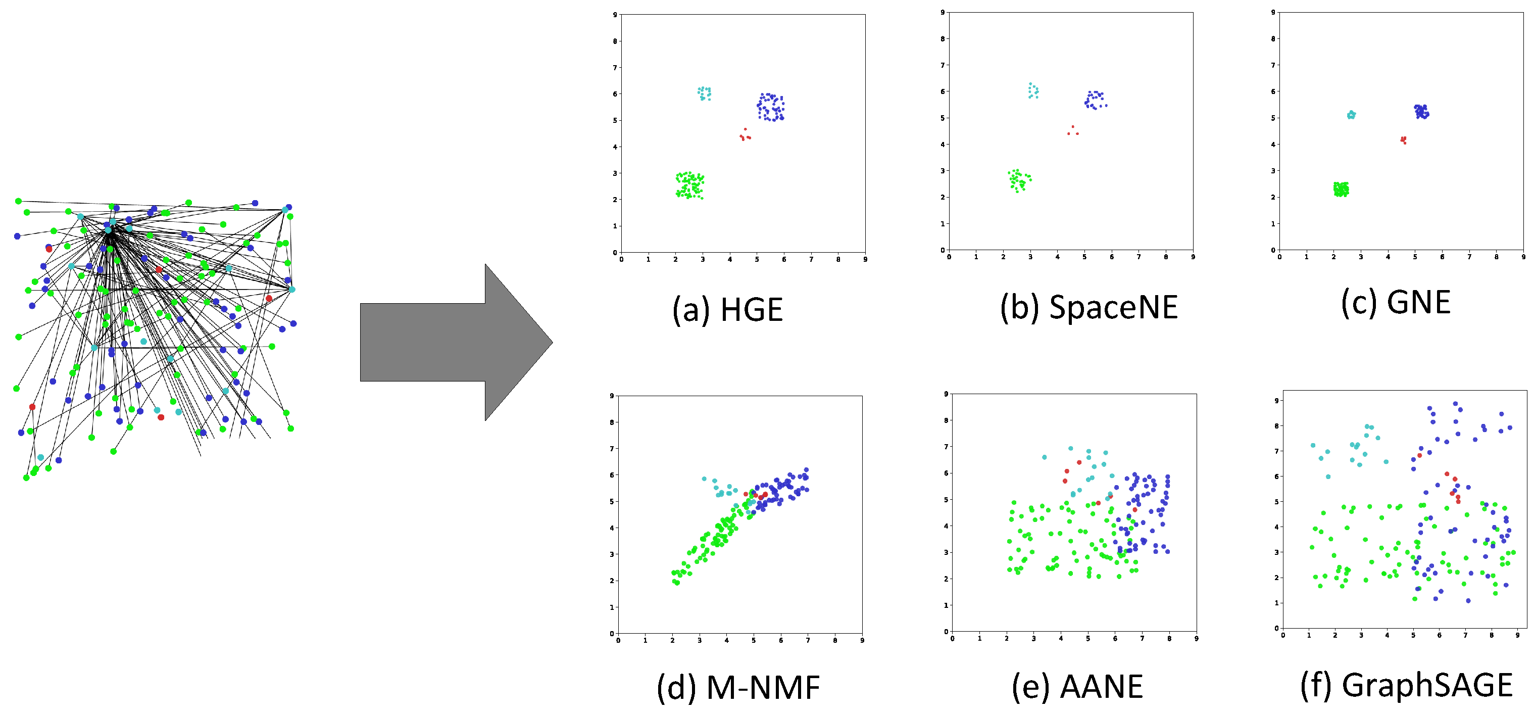
6.3. Performance of Network Visualization of the HGE Model

Network visualization is also one of the most important means to detect the quality of the learned embedding. Network visualization maps a network into two-dimensional space. In this section, for better visualization, we visualize a sub-network which is selected from the BlogCatalog dataset with 175 nodes and 150 edges.

From Figure 6, we find that our HGE model preserves the default hierarchical structure, and distributes the nodes of each layer more uniformly in a fan-shaped area.

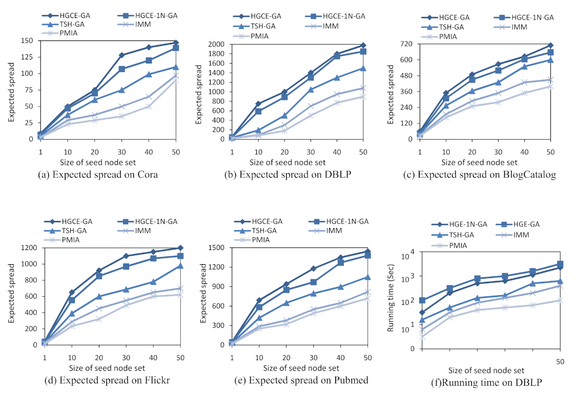
6.4. Overall Performance of HGE-GA Algorithm

We adopt the metric of expected spread to evaluate the overall performance of all influence maximization algorithms. To compare the proposed HGE-GA algorithm with the baselines, we change the size of the seed node set K to be 1, 20, 30, 40, and 50. The experimental results are reported in Figure 7a–e. It can be observed from Figure 7a–e that:

(1) The expected spread increases for all algorithms when enlarging the size of the seed node set. The proposed HGE-GA algorithm outperforms all the baselines significantly for all seed sizes on the five datasets. For instance, on the Pubmed dataset, when the seed set size $K = 50$, the value of the expected spread of the proposed HGE-GA algorithm is 1445, compared with 721 for PMIA, 819 for IMM, 1052 for TSH-GA, and 1384 for HGE-1N-GA;

(2) On all five datasets, all of the attribute-related algorithms, TSH-GA, HGE-1N-GA and HGE-GA, outperform the non-attribute-related algorithms, PMIA and IMM, in terms of the performance of the expected spread. This is because the PMIA and IMM algorithms do not have the step of predicting the influence probability of node pairs, with influence probability being set uniformly. Moreover, this demonstrates that homophily is a cause of similar behaviors and is useful for predicting future behaviors of users. Consequently, the expected spread can be increased obviously when node attributes are taken into account in modeling;

(3) HGE-1N-GA and HGE-GA outperform TSH-GA on the five datasets for the metric of expected spread. The reason is that HGE-1N-GA and HGE-GA consider the general network structure, hierarchical network structure as well as node attributes to learn users’ latent feature representations for predicting the influence probability of node pairs, but TSH-GA uses hand-crafted rules to extract the features of users’ interactions, network structure and node homophily, heavily depending on the domain expert’s knowledge and without considering hierarchical network structure;

(4) The expected spread of HGE-GA is superior than HGE-1N-GA. The reason is obvious: HGE-1N-GA uses the one-normal form to compute the similarity of two nodes, while HGE-GA leverages the two-normal form to compute similarity, which can capture the relationships between nodes better.

The running times of all algorithms are reported in Figure 7f. This figure only presents the experimental results on the DBLP dataset due to space constraints. Please note that the DBLP dataset is the biggest dataset in the five datasets considering both the number of nodes and the number of edges. Similar trends of performance of the algorithms are found for the other four datasets. From Figure 7b,f, it can be observed that, for the DBLP dataset, compared with the baseline algorithms, the proposed algorithm, HGE-GA, obtains a better performance of the expected spread by spending more time. However, in general, the proposed algorithm HGE-GA spends an acceptable running time to obtain 54.5%, 45.5%, 24.2% more expected spread, respectively, than the PMIA, IMM and TSH-GA algorithms when the seed set size K is set to 50.

7. Conclusions

In this paper, we study the problem of influence maximization in attributed social networks, assuming the influence strength is directly unobservable. From the deep learning perspective, we formulate the problem and propose a hierarchical generative embedding model, HGE, to map nodes into latent space automatically, incorporating hierarchical community structure, node attributes and general network structure into a unified deep generative framework. Then, with the learned latent representation of each node, we propose a HGE-GA algorithm to predict influence strength and find the seed node set. The experimental results show that the proposed HGE model is able to learn representations of nodes in attributed networks far more effectively than state-of-the-art models in terms of several downstream applications, such as vertex classification, link prediction and network visualization. It is also verified by the experimental results that the proposed HGE-GA algorithm significantly outperforms the state-of-the-art algorithms for influence maximization in attributed social networks.

As to future work, we intend to extend our HGE model to temporal attributed networks, which is more challenging because this kind of attributed network evolves over time and vertexes need to be embedded dynamically.

References

- Huang, H.; Meng, Z.; Shen, H. Competitive and complementary influence maximization in social network: A follower’s perspective. Knowl.-Based Syst. 2021, 213, 106600. [Google Scholar] [CrossRef]
- Fedushko, S.; Peráček, T.; Syerov, Y.; Trach, O. Development of Methods for the Strategic Management of Web Projects. Sustainability 2021, 13, 742. [Google Scholar] [CrossRef]
- Kempe, D.; Kleinberg, J.; Tardos, É. Maximizing the spread of influence through a social network. In Proceedings of the Ninth ACM SIGKDD International Conference on Knowledge Discovery and Data Mining, Washington, DC, USA, 24–27 August 2003; pp. 137–146. [Google Scholar]
- Pei, S.; Morone, F.; Makse, H.A. Theories for influencer identification in complex networks. In Complex Spreading Phenomena in Social Systems; Springer: Berlin/Heidelberg, Germany, 2018; pp. 125–148. [Google Scholar]
- Sheshar, S.; Srivastva, S.D.; Verma, M.; Singh, J. Influence Maximization Frameworks, Performance, Challenges and Directions on Social Network: A Theoretical Study. J. King Saud-Univ.-Comput. Inf. Sci. 2021; in press. [Google Scholar] [CrossRef]
- Leskovec, J.; Krause, A.; Guestrin, C.; Faloutsos, C.; VanBriesen, J.; Glance, N. Cost-effective outbreak detection in networks. In Proceedings of the 13th ACM SIGKDD International Conference on Knowledge Discovery and Data Mining, San Jose, CA, USA, 12–15 August 2007; pp. 420–429. [Google Scholar]
- Chen, W.; Wang, Y.; Yang, S. Efficient influence maximization in social networks. In Proceedings of the 15th ACM SIGKDD International Conference on Knowledge Discovery and Data Mining, Paris, France, 28 June–1 July 2009; pp. 199–208. [Google Scholar]
- Goyal, A.; Lu, W.; Lakshmanan, L.V. Celf++ optimizing the greedy algorithm for influence maximization in social networks. In Proceedings of the 20th International Conference Companion on World Wide Web, Hyderabad, India, 28 March–1 April 2011; pp. 47–48. [Google Scholar]
- Tang, Y.; Shi, Y.; Xiao, X. Influence maximization in near-linear time: A martingale approach. In Proceedings of the 2015 ACM SIGMOD International Conference on Management of Data, Melbourne, VIC, Australia, 31 May–4 June 2015; pp. 1539–1554. [Google Scholar]
- Cheng, S.; Shen, H.; Huang, J.; Zhang, G.; Cheng, X. Staticgreedy: Solving the scalability-accuracy dilemma in influence maximization. In Proceedings of the 22nd ACM International Conference on Information & Knowledge Management, Francisco, CA, USA, 27 October–1 November 2013; pp. 509–518. [Google Scholar]
- Galhotra, S.; Arora, A.; Roy, S. Holistic influence maximization: Combining scalability and efficiency with opinion-aware models. In Proceedings of the 2016 International Conference on Management of Data, San Francisco, CA, USA, 26 June–1 July 2016; pp. 743–758. [Google Scholar]
- Chen, W.; Wang, C.; Wang, Y. Scalable influence maximization for prevalent viral marketing in large-scale social networks. In Proceedings of the 16th ACM SIGKDD International Conference on Knowledge Discovery and Data Mining, Washington, DC, USA, 24–28 July 2010; pp. 1029–1038. [Google Scholar]
- Jiang, Q.; Song, G.; Gao, C.; Wang, Y.; Si, W.; Xie, K. Simulated annealing based influence maximization in social networks. In Proceedings of the AAAI Conference on Artificial Intelligence, San Francisco, CA, USA, 7–11 August 2011; Volume 25. [Google Scholar]
- Hu, Z.; Yao, J.; Cui, B.; Xing, E. Community level diffusion extraction. In Proceedings of the 2015 ACM SIGMOD International Conference on Management of Data, Melbourne, VIC, Australia, 31 May–4 June 2015; pp. 1555–1569. [Google Scholar]
- Huang, H.; Shen, H.; Meng, Z.; Chang, H.; He, H. Community-based influence maximization for viral marketing. Appl. Intell. 2019, 49, 2137–2150. [Google Scholar] [CrossRef]
- Shaghaghian, S.; Coates, M. Bayesian inference of diffusion networks with unknown infection times. In Proceedings of the 2016 IEEE Statistical Signal Processing Workshop (SSP), Palma de Mallorca, Spain, 26–29 June 2016; pp. 1–5. [Google Scholar]
- Barbieri, N.; Bonchi, F.; Manco, G. Topic-aware social influence propagation models. Knowl. Inf. Syst. 2013, 37, 555–584. [Google Scholar] [CrossRef]
- Huang, H.; Meng, Z.; Liang, S. Recurrent neural variational model for follower-based influence maximization. Inf. Sci. 2020, 528, 280–293. [Google Scholar] [CrossRef]
- Qiu, J.; Tang, J.; Ma, H.; Dong, Y.; Wang, K.; Tang, J. Deepinf: Social influence prediction with deep learning. In Proceedings of the 24th ACM SIGKDD International Conference on Knowledge Discovery & Data Mining, London, UK, 19–23 August 2018; pp. 2110–2119. [Google Scholar]
- Zhou, F.; Jiao, R.J.; Lei, B.Y. A linear threshold-hurdle model for product adoption prediction incorporating social network effects. Inf. Sci. 2015, 307, 95–109. [Google Scholar] [CrossRef]
- Kamarthi, H.; Vijayan, P.; Wilder, B.; Ravindran, B.; Tambe, M. Influence Maximization in Unknown Social Networks: Learning Policies for Effective Graph Sampling. In Proceedings of the 19th International Conference on Autonomous Agents and MultiAgent Systems, Auckland, New Zealand, 9–13 May 2020; pp. 575–583. [Google Scholar]
- Mikolov, T.; Chen, K.; Corrado, G.; Dean, J. Efficient estimation of word representations in vector space. arXiv 2013, arXiv:1301.3781. [Google Scholar]
- Perozzi, B.; Al-Rfou, R.; Skiena, S. Deepwalk: On learning of social representations. In Proceedings of the 20th ACM SIGKDD International Conference on Knowledge Discovery and Data Mining, New York, NY, USA, 24–27 August 2014; pp. 701–710. [Google Scholar]
- Grover, A.; Leskovec, J. node2vec: Scalable feature learning for networks. In Proceedings of the 22nd ACM SIGKDD International Conference on Knowledge Discovery and Data Mining, San Francisco, CA, USA, 13–17 August 2016; pp. 855–864. [Google Scholar]
- Tang, J.; Qu, M.; Wang, M.; Zhang, M.; Yan, J.; Mei, Q. Line: Large-scale information network embedding. In Proceedings of the 24th International Conference on World Wide Web, Florence, Italy, 18–22 May 2015; pp. 1067–1077. [Google Scholar]
- Wang, D.; Cui, P.; Zhu, W. Structural deep network embedding. In Proceedings of the 22nd ACM SIGKDD International Conference on Knowledge Discovery and DATA Mining, San Francisco, CA, USA, 13–17 August 2016; pp. 1225–1234. [Google Scholar]
- Wang, X.; Cui, P.; Wang, J.; Pei, J.; Zhu, W.; Yang, S. Community preserving network embedding. In Proceedings of the Thirty-First AAAI Conference on Artificial Intelligence, San Francisco, CA, USA, 4–9 February 2017. [Google Scholar]
- Jia, Y.; Zhang, Q.; Zhang, W.; Wang, X. Communitygan: Community detection with generative adversarial nets. In Proceedings of the World Wide Web Conference, San Francisco, CA, USA, 13–17 May 2019; pp. 784–794. [Google Scholar]
- Li, Y.; Wang, Y.; Zhang, T.; Zhang, J.; Chang, Y. Learning network embedding with community structural information. In Proceedings of the 28th International Joint Conference on Artificial Intelligence, Macao, China, 10–16 August 2019; pp. 2937–2943. [Google Scholar]
- Goodfellow, I.; Pouget-Abadie, J.; Mirza, M.; Xu, B.; Warde-Farley, D.; Ozair, S.; Courville, A.; Bengio, Y. Generative adversarial nets. In Proceedings of the Advances in Neural Information Processing Systems, Montreal, QC, USA, 8–13 December 2014; pp. 2672–2680. [Google Scholar]
- Yang, J.; Leskovec, J. Community-affiliation graph model for overlapping network community detection. In Proceedings of the 2012 IEEE 12th International Conference on Data Mining, Brussels, Belgium, 10–13 December 2012; pp. 1170–1175. [Google Scholar]
- Clauset, A.; Moore, C.; Newman, M.E. Structural inference of hierarchies in networks. In Proceedings of the ICML Workshop on Statistical Network Analysis, Pittsburgh, PA, USA, 29 June 2006; pp. 1–13. [Google Scholar]
- Du, L.; Lu, Z.; Wang, Y.; Song, G.; Wang, Y.; Chen, W. Galaxy Network Embedding: A Hierarchical Community Structure Preserving Approach. In Proceedings of the IJCAI, Stockholm, Sweden, 13–19 July 2018; pp. 2079–2085. [Google Scholar]
- Sales-Pardo, M.; Guimera, R.; Moreira, A.A.; Amaral, L.A.N. Extracting the hierarchical organization of complex systems. Proc. Natl. Acad. Sci. USA 2007, 104, 15224–15229. [Google Scholar] [CrossRef] [PubMed] [Green Version]
- Ma, J.; Cui, P.; Wang, X.; Zhu, W. Hierarchical taxonomy aware network embedding. In Proceedings of the 24th ACM SIGKDD International Conference on Knowledge Discovery & Data Mining, London, UK, 19–23 August 2018; pp. 1920–1929. [Google Scholar]
- Long, Q.; Wang, Y.; Du, L.; Song, G.; Jin, Y.; Lin, W. Hierarchical Community Structure Preserving Network Embedding: A Subspace Approach. In Proceedings of the 28th ACM International Conference on Information and Knowledge Management, Beijing, China, 3–7 November 2019; pp. 409–418. [Google Scholar]
- Ma, Y.; Ren, Z.; Jiang, Z.; Tang, J.; Yin, D. Multi-Dimensional Network Embedding with Hierarchical Structure. In Proceedings of the Eleventh ACM International Conference on Web Search and Data Mining 2018, Los Angeles, CA, USA, 5–9 February 2018; pp. 387–395. [Google Scholar]
- Nickel, M.; Kiela, D. Poincaré embeddings for learning hierarchical representations. In Proceedings of the Advances in Neural Information Processing Systems, Long Beach, CA, USA, 4–9 December 2017; pp. 6338–6347. [Google Scholar]
- Bojchevski, A.; Günnemann, S. Deep Gaussian Embedding of Graphs: Unsupervised Inductive Learning via Ranking. In Proceedings of the International Conference on Learning Representations, Vancouver, BC, Canada, 30 April–3 May 2018. [Google Scholar]
- Hamilton, W.L.; Ying, Z.; Leskovec, J. Inductive Representation Learning on Large Graphs. In Proceedings of the Advances in Neural Information Processing Systems 30: Annual Conference on Neural Information Processing Systems, Long Beach, CA, USA, 4–9 December 2017; pp. 1024–1034. [Google Scholar]
- Huang, X.; Li, J.; Hu, X. Accelerated Attributed Network Embedding. In Proceedings of the 2017 SIAM International Conference on Data Mining, Houston, TX, USA, 27–29 April 2017; pp. 633–641. [Google Scholar]
Figure 1.
A toy example of social influence. The seed nodes are ,,, represented in black, and the nodes influenced by the seed nodes are in gray.
Figure 2.
The correspondence between the general attributed network and the hierarchical latent space.
Figure 3.
Overview of the system architecture.
Figure 4.
Illustration of vertexes at different levels having different granularity features.
Figure 5.
A case for which methods based on the inner product cannot capture the relationship between nodes. As we can see, the relationship between and and the relationship between node and can not be captured.
Figure 6.
The experimental results of network visualization in two-dimensional space.
Figure 7.
Expected spread and running time with different sizes of seed node set K.