A Pre-Scheduling Mechanism in LTE Handover for Streaming Video

Abstract

This paper focuses on downlink packet scheduling for streaming video in Long Term Evolution (LTE). As a hard handover is adopted in LTE and has the period of breaking connection, it may cause a low user-perceived video quality. Therefore, we propose a handover prediction mechanism and a pre-scheduling mechanism to dynamically adjust the data rates of transmissions for providing a high quality of service (QoS) for streaming video before new connection establishment. Advantages of our method in comparison to the exponential/proportional fair (EXP/PF) scheme are shown through simulation experiments.

1. Introduction

For improving a low transmission rate of the 3G technologies, LTE (Long Term Evolution) was designed as a next-generation wireless system by the 3rd Generation Partnership Project (3GPP) to enhance the transmission efficiency in mobile networks [1,2]. LTE is a packet-based network, and information coming from many users is multiplexed in time and frequency domains. Many different downlink packet schedulers are proposed and utilized to optimize the network throughput [3,4]. There are three typical strategies: (1) round robin (RR), (2) maximum rate (MR) and (3) proportional fair (PF). The RR scheme is a fair scheduler, in which every user has the same priority for transmissions, but the RR scheme may lead to low throughput. MR aims to maximize the system throughput by selecting the user with the best channel condition (the largest bandwidth) such as by comparing the signal to noise ratio (SNR) values. Moreover, the PF mechanism utilizes link adaptation (LA) technology. It compares the current channel rate with the average throughput for each user and selects the one with the largest value. However, these methods only consider non-real-time data transmissions. Therefore, some packet schedulers are proposed based on PF algorithm for real-time data transmissions [5,6]. In one study [5], a Maximum-Largest Weighted Delay First (M-LWDF) algorithm is proposed. In addition to data rate, M-LWDF takes weights of the head-of-line (HOL) packet delay (between current time and the arrival time of a packet) into consideration. It also combines HOL packet delay with the PF algorithm to achieve a good throughput and fairness. In another study [6], an exponential/proportional fair (EXP/PF) is proposed. EXP/PF is designed for both real-time and non-real time traffic. Compared to M-LWDF, the average HOL packet delay is also taken into account. Because of the consideration of packet delay time, M-LWDF and EXP/PF can achieve higher performance than the other mechanisms in real-time transmissions [7]. Other schedulers for real-time data transmissions are as follows. In one study [8], two semi-persistent scheduling (SPS) algorithms are proposed to achieve a high reception ratio in real-time transmission. It also utilizes wide-band time-average signal-to-interference-plus-noise ratios (SINR) information for physical resource blocks (PRBs) allocation to improve the performance of large packet transmissions. In another study [9], the mechanism provides fairness-aware downlink scheduling for different types of packets. Three queues are utilized for data transmission arrangement according to the different priority needs. If a user is located near cell′s edge, his services may not be accepted. This may still cause starvation and fairness problems. In yet another study [10], a two-level downlink scheduling is proposed. The mechanism utilizes a discrete control theory and a proportional fair scheduler in upper-level and lower level, respectively. Results show that the strategy is suitable for real-time video flows. However, most schedulers do not improve low transmission rates during the LTE handover procedure and meet the needs of video quality for users.

The scalable video coding (SVC) is a key technology for spreading streaming video over the internet. SVC can dynamically adapt the video quality to the network state. It divides a video frame into one base layer (BL) and number of enhancement layers (ELs). The BL includes the most important information of the original frame and must be used by a user for playing a video frame. Although ELs can be added to the base layer to further enhance the quality of coded video, it may not be essential. Therefore, in this paper, we propose a pre-scheduling mechanism to determine the transmission rates of BL and EL, especially focusing on the BL transmissions, before a new connection handover for providing high quality of service (QoS) for streaming video.

2. Pre-Scheduling Mechanism

Our proposed mechanism is divided into two phases: (1) handover prediction and (2) pre-scheduling mechanism.

2.1. Handover Prediction

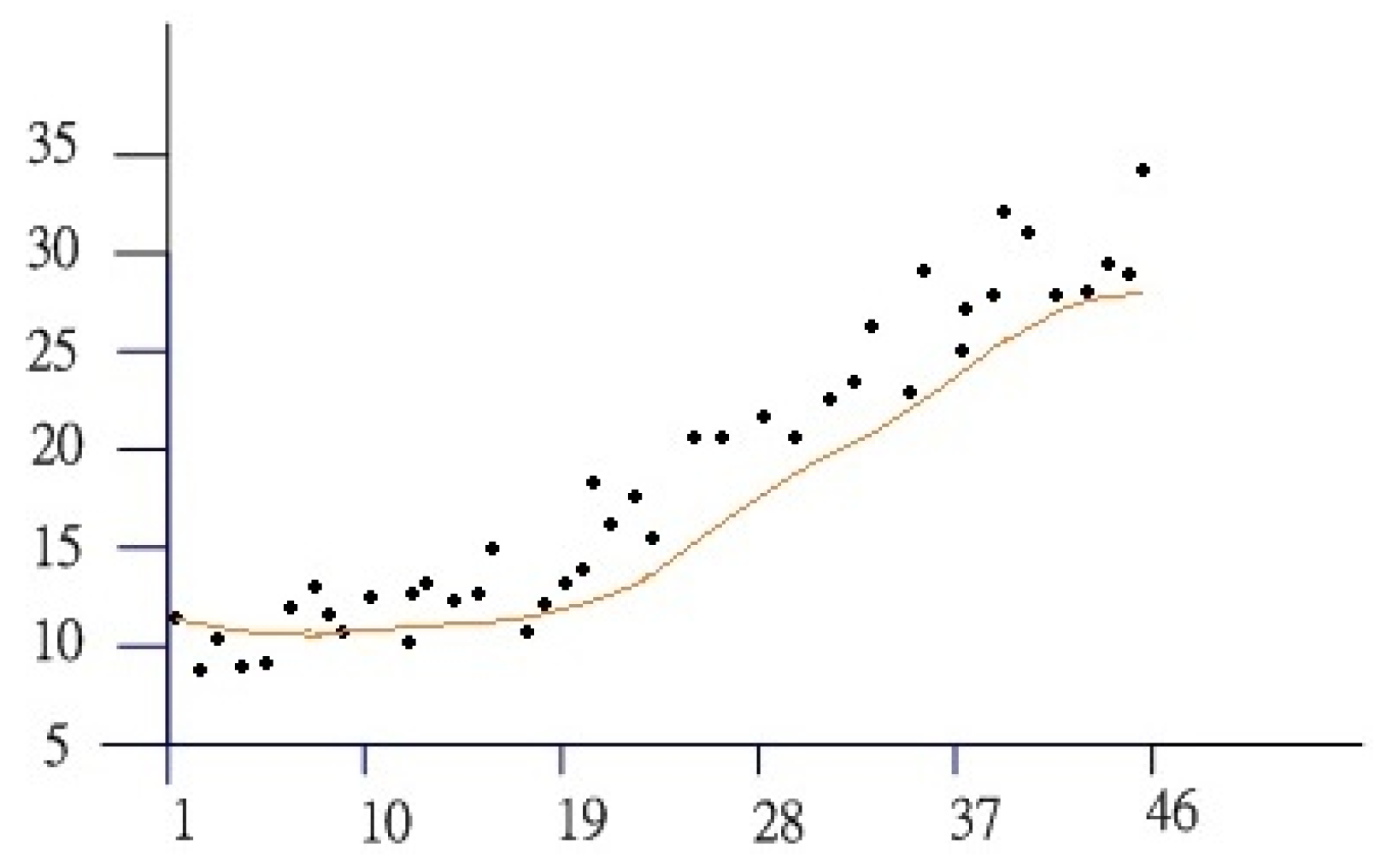
Handover determination generally depends on the degradation of the Reference Signal Receiving Power (RSRP) from the base station (eNodeB). When the threshold value is reached, a handover procedure is triggered. Many works have focused on handover decisions [11,12,13,14,15,16]. In this paper, user measures RSRP periodically with neighbor eNodeBs. In addition, we use exponential smoothing (ES) to remove high-frequency random noise (Figure 1), where α is a smoothing constant. Then, we incorporate a linear regression model with RSRP values to predict time-to-trigger (TTT) for handover.

The linear regression equation can be simply expressed as follows:

$${\widehat{P}}_i=a+b{t}_i,i=1,2,\dots ,n$$

(1)

where ${\widehat{P}}_i$ is the predictive value of RSRP at time $t_i$, and $a$ and b are coefficients of the linear regression equation. Then, we use the least squares (LS) method to deduce a and b. The method of LS is a standard solution to estimate the coefficient in linear regression analysis.

Let the sum of the residual squares be S, that is

$$S={{\displaystyle \sum }}_{i=1}^n{\left[P_i-\left(a+b{t}_i\right)\right]}^2$$

(2)

where $P_i$ is the measured value of RSRP at time $t_i$. The least squares method is to try to find the minimum of S, and then the minimum of S is determined by calculating the partial derivatives.

$$\text{Let}\{\begin{array}{c}\frac{\partial p}{\partial a}={\displaystyle \sum }_{i=1}^{n}2\left[P_i-\left(a+b{t}_i\right)\right]\left(-1\right)=0\\ \frac{\partial p}{\partial b}={\displaystyle \sum }_{i=1}^{n}2\left[P_i-\left(a+b{t}_i\right)\right]\left(-t_i\right)=0\end{array}$$

(3)

Finally we can get

$$\{\begin{array}{c}a=\overline{P}-b\overline{t}\\ \\ b=\frac{{{\displaystyle \sum }}_{i=1}^n{t}_i{P}_i–n\overline{TP}}{{{\displaystyle \sum }}_{i=1}^n{t}_i{}^2-n{\overline{T}}^2}\end{array}$$

(4)

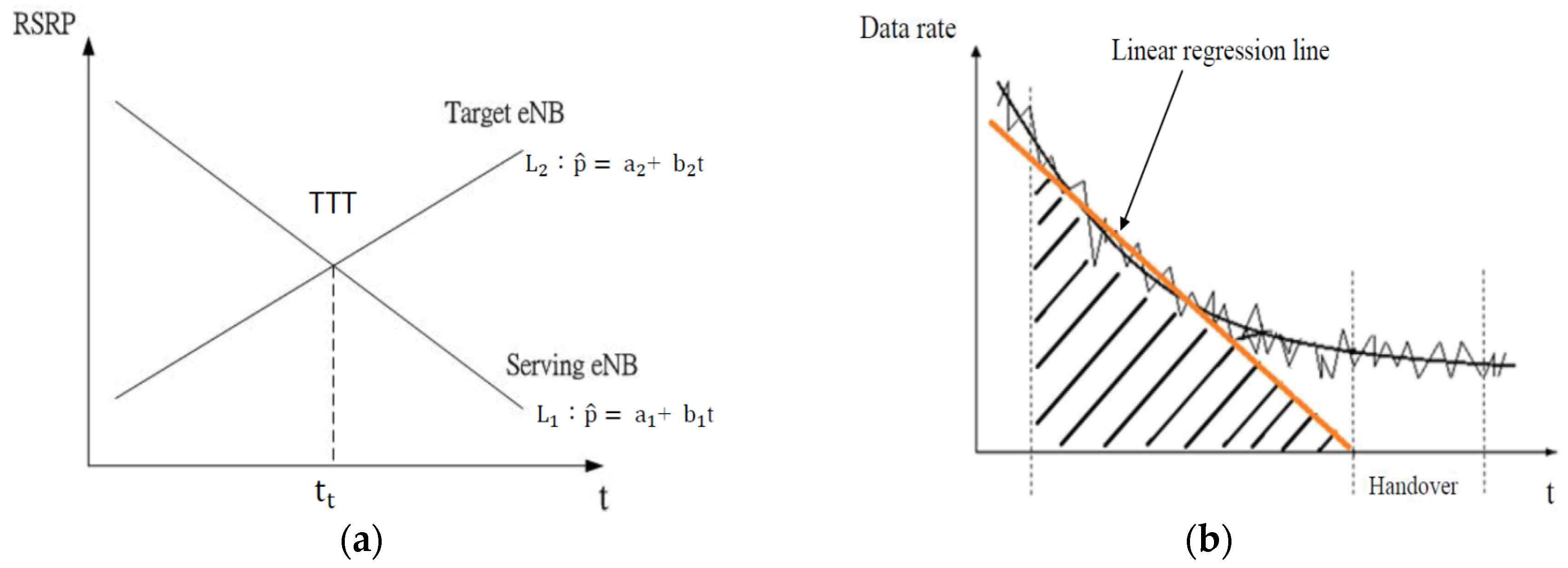
where $\overline{T}=\frac{{{\displaystyle \sum }}_{i=1}^n{t}_i}{n}$ and $\overline{P}=\frac{{{\displaystyle \sum }}_{i=1}^n{P}_i}{n}$. If there are several neighbor eNodes, we select the eNodeB with the maximum variation of RSRP (maximum slope) as target eNodeB. In Figure 2a, we can see that while ${\text{RSRP}}_{\text{SeNB}}={\text{RSRP}}_{\text{TeNB}}$, the handover procedure is triggered. We have trigger time $t_{\mathrm{t}}=\frac{a_1-a_2}{b_2-b_1}$.

2.2. Pre-Scheduling Mechanism

The BL is necessary for the video stream to be decoded. ELs are utilized to improve stream quality. Therefore, for high QoS for video streaming, we calculate the total number of BL that is required in a handover period for maintaining high QoS for video streaming.

$$N_{BL}=\left(t_r+t_{ho}+t_n\right)\times K_s\times m$$

(5)

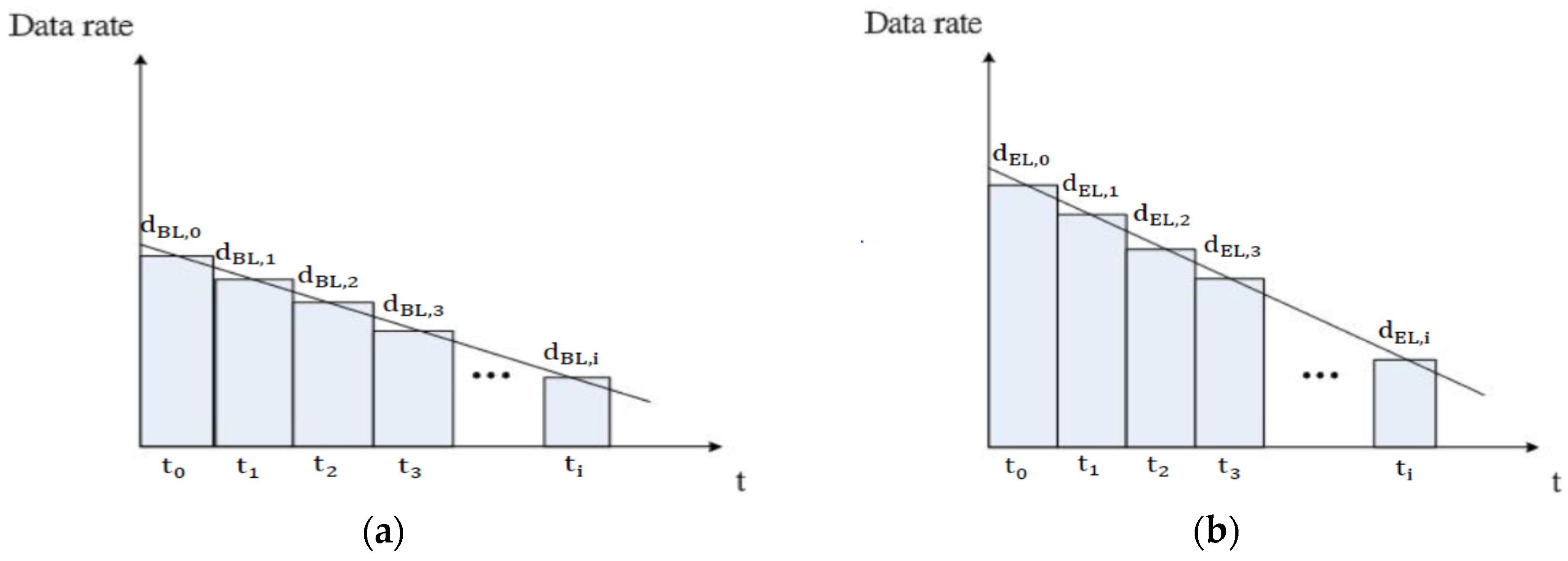
where $t_r$ is the time interval from scheduling to starting handover (pre-scheduling time for handover). The starting time of scheduling is adjustable, and we will evaluate it in our simulation later. $t_{ho}$ is the time during handover procedure. $t_n$ is the delay time before new transmission (preparation time of scheduling with new eNodeB). $K_s$ is the required number of video frames per second and $\mathrm{m}$ is the number of BL that is needed in each video frame. In Figure 2b, according to transmission data rate of the serving eNodeB, we construct a linear regression line $d_x\left(t\right)$. Then, the amount of BL’s data (transmitted from serving eNodeB and stored in the buffer of users) before handover has to be no less than$N_{BL}$.

$${{\displaystyle \int }}_{t_{now}}^{t_{handover}}{d}_x\left(t\right)dt\ge N_{BL}$$

(6)

where $t_{handover}$ is the TTT for handover. In the above inequality, the left part is the amount of data that the serving eNodeB can transmit before handover. According to the serving eNodeB capacity of transmission, we can dynamically adjust the transmission rate between BL and ELs. In Equation (6), while the inequality does not hold, it means the serving eNodeB cannot provide enough data for BL for maintaining high QoS for video streaming. Accordingly, the serving eNodeB merely transmits data for BL. On the contrary, while the inequality holds, the serving eNodeB can provide the data of BL and ELs simultaneously for desired quality of video service. In the following, we describe our mechanism of data rate adjustment between BL and ELs. The transmission rates of the BL and ELs are decreasing because the RSRP is degrading between the previous serving eNodeB and user. Hence, by the regression line $d_x\left(t\right)$, we can define the total descent rate s (slope) of transmissions as

$$s=\frac{\Delta \mathrm{y}}{\Delta \mathrm{x}}$$

(7)

In Figure 3, because of the decreasing RSRP, the transmission rates of BL and EL are also decreasing with time unit respectively. Then, we let per time unit be $t_{unit}$, that is,

$$t_0=t_1=t_2=t_3=\dots =t_i=t_{unit}$$

(8)

Because of the limitative transmission rate of the serving eNodeB during a certain time interval, we have

$$t_{unit}·\left(d_{BL,i}+d_{EL,i}\right)\le {{\displaystyle \int }}_{0+t_{unit}·i}^{0+t_{unit}·\left(i+1\right)}{d}_x\left(t\right)dt$$

(9)

where $d_{BL,i}$ and $d_{EL,i}$ are the transmitted number of BL and ELs during time interval $t_i$, respectively. In Equation (9), the total transmitted number for streaming video (left part) is necessarily less than or equal to the total number of data the serving eNodeB can provide (right part). Thus, the total descent rate of transmission per $t_{unit}$ can be calculated as $s·t_{unit}$. In this paper, for high QoS for video streaming, BL data has high priority for transmission. Furthermore, to achieve dynamically adjusting the transmission rate between BL and EL, we define the descent rate as

$$K_i=\frac{d_{EL,0}}{d_{BL,0}}$$

(10)

$K_i$ is the proportion of the transmission rate between EL and BL during the time interval. That is, the transmission rate of BL is written as

$$s·t_{unit}·\frac{1}{K_i+1}$$

(11)

Then, we calculate the transmission rate of BL in each time unit

$$\begin{array}{c}{d}_{BL,0}\\ d_{BL,1}=d_{BL,0}+s·t_{unit}·\frac{1}{K_i+1}\\ d_{BL,2}=d_{BL,1}+s·t_{unit}·\frac{1}{K_i+1}=d_{BL,0}+2·s·t_{unit}·\frac{1}{K_i+1}\\ d_{BL,3}=d_{BL,2}+s·t_{unit}·\frac{1}{K_i+1}=d_{BL,0}+3·s·t_{unit}·\frac{1}{K_i+1}\\ d_{BL,i}=d_{BL,0}+i·s·t_{unit}·\frac{1}{K_i+1}=d_{BL,0}+\frac{i·s·t_{unit}}{K_i+1}\end{array}$$

(12)

Finally, we can calculate the total transmitted BL data from time $t_0$ to $t_r$ (pre-scheduling time before handover)

$$\begin{array}{l}{t}_{unit}·\left[d_{BL,0}+d_{BL,1}+d_{BL,2}+\dots +d_{BL,i}\right]\\ =t_{unit}·\left[d_{BL,0}+d_{BL,1}+d_{BL,2}+\dots +d_{BL,\left(\frac{t_r}{t_{unit}}-1\right)}\right]\\ =t_{unit}·\left[d_{BL,0}+d_{BL,0}+\frac{s·t_{unit}}{K_i+1}+d_{BL,0}+2·\frac{s·t_{unit}}{K_i+1}+\dots \right]\\ =t_{unit}·\left[\frac{t_r}{t_{unit}}·d_{BL,0}+\frac{\left(\frac{t_r}{t_{unit}}-1+1\right)·\left(\frac{t_r}{t_{unit}}-1\right)}{2}·\frac{s·t_{unit}}{K_i+1}\right]\\ =t_{unit}·\left[\frac{t_r}{t_{unit}}·d_{BL,0}+\frac{t_r·s·\left(\frac{t_r}{t_{unit}}-1\right)}{2·\left(K_i+1\right)}\right]\\ =t_r·d_{BL,0}+\frac{t_r·s·\left(t_r-t_{unit}\right)}{2·\left(K_i+1\right)}\end{array}$$

(13)

The total transmission number of BL is required to be no less than the number of BL for maintaining high QoS for video streaming, that is,

$$t_r·d_{BL,0}+\frac{t_r·s·\left(t_r-t_{unit}\right)}{2·\left(K_i+1\right)}\ge \left(t_r+t_{ho}+t_n\right)\times K_s\times m$$

(14)

Finally, we have

$$d_{BL,0}\ge -\frac{s·\left(t_r-t_{unit}\right)}{2·\left(K_i+1\right)}+\left(1+\frac{t_{ho}+t_n}{t_r}\right)\times K_s\times m$$

(15)

In Equation (15), because $s,t_{unit},t_{ho},t_n,K_s$, and m are pre-defined values, we only consider $K_i,t_r\text{ and }{d}_{BL,0}$in the following simulations. In this paper, for maintaining high QoS for video streaming, the BL data transmission must be given precedence over the EL data. Therefore, $d_{BL,0}$ value can be determined in advance. Due to the limitation of the total number of data the serving eNodeB can provide, $d_{EL,0}$ also can be determined. Eventually, $K_i$ is decided for BL and EL transmissions. A sufficient $t_r$ represents that more pre-scheduling time can be utilized for transmitting EL data to enhance video quality. On the contrary, BL transmissions are increased to achieve high QoS for video streaming.

Research manuscripts reporting large datasets that are deposited in a publicly available database should specify where the data have been deposited and provide the relevant accession numbers. If the accession numbers have not yet been obtained at the time of submission, please state that they will be provided during review. They must be provided prior to publication.

3. Performance Evaluation

3.1. The Effect of the Prediction Mechanism

We evaluate our scheme through simulations implemented in the LTE-Sim [17] simulator. LTE-Sim can provide a thorough performance verification of LTE networks. We also utilize Video Trace Library [18] with LTE-Sim to present real-time streaming video for network performance evaluations. The simulation parameters are summarized as

Table 1. Parameters of simulation.

Parameter	Values
Simulation Time	100 s
Simulation Rounds	100
Cell Radius	1 km
Number of User Equipments (Ues) (per cell)	30, 40, 50
Velocity of UEs (km/h)	30, 120
UE Application Flows	Video Application
Modulation and Coding Scheme	QPSK, 16QAM, 64QAM
Number of Cells	7
Number of eNodeB	7
Bandwidth	10 MHz
Number of PRBs	50 (12 Subcarriers/PRB)
Transmission Time Interval	0.5 ms/slot
	1 ms/subframe
	10 ms radio frame/TTI
Mobility Model of UEs	Random Direction

.

The accuracy of handover prediction affects the pre-scheduling time ($t_r$) for BL and EL transmission rate. In Figure 4, as user equipments (UEs) velocity is 30 km/h and the actual TTT of handover is 79.924 s, we can have an error rate smaller than 0.8% while the prediction is made after 59 s. On the other hand, as UE velocity is 120 km/h, the actual TTT of handover is 25.981 s and the error rate can be contained smaller than 0.5% as the prediction is made after 15 s. Faster UE results in shorter pre-scheduling time for transmissions accordingly. On the contrary, more pre-scheduling time can be used for transmissions. Therefore, we can adaptively trigger the pre-scheduling procedure and adjust the transmission rates between BL and ELs with limited resource.

3.2. Base Layer Adjustment

Our goal is to provide high QoS for video streaming before new connection establishment. Since BL includes the most basic data for playing the video, for this reason, BL is needed to transmit in advance. In the following, we discuss the simulation result of BL adjustment.

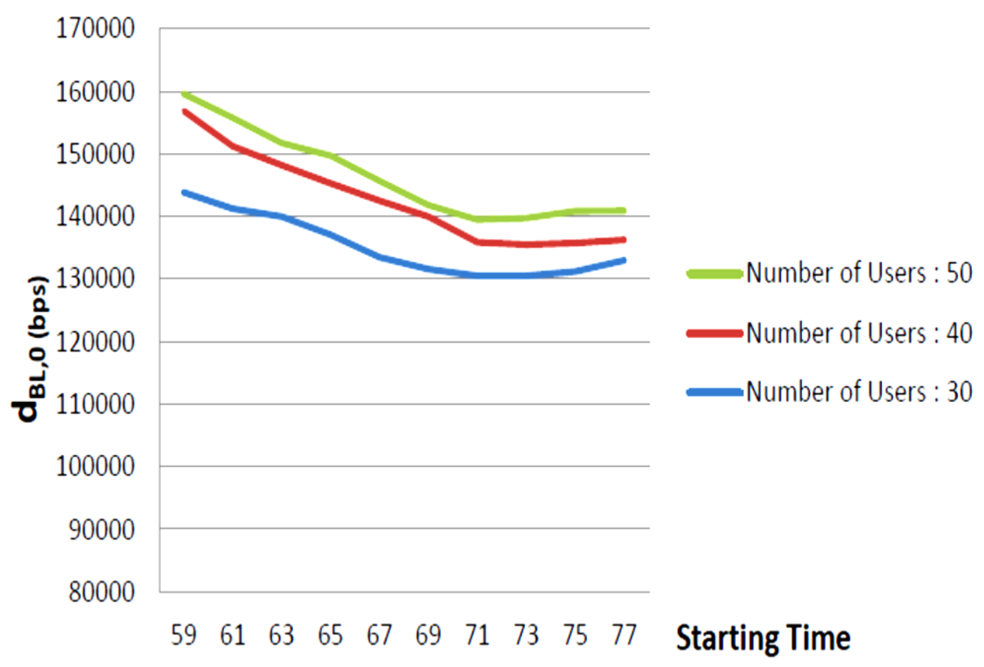
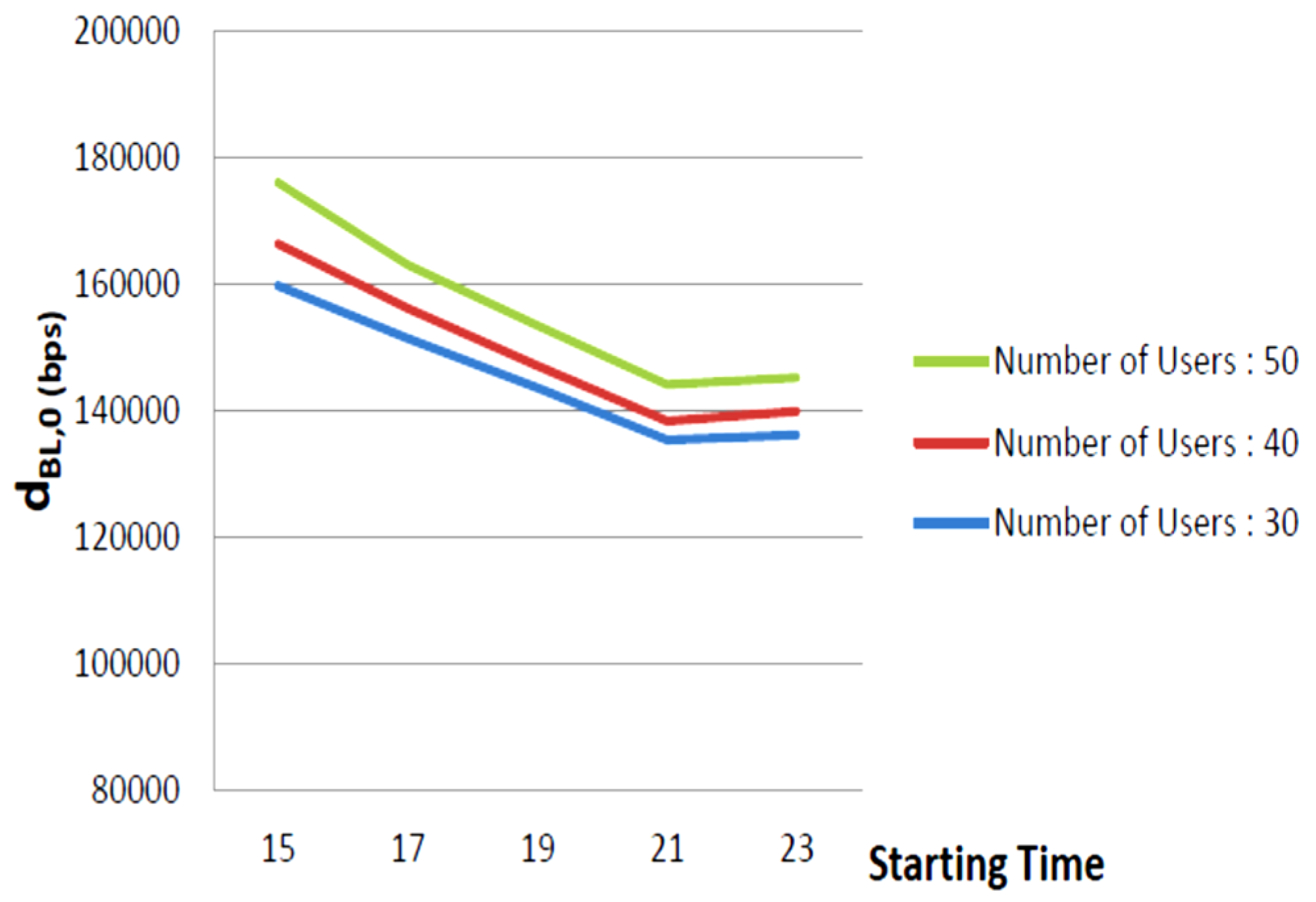
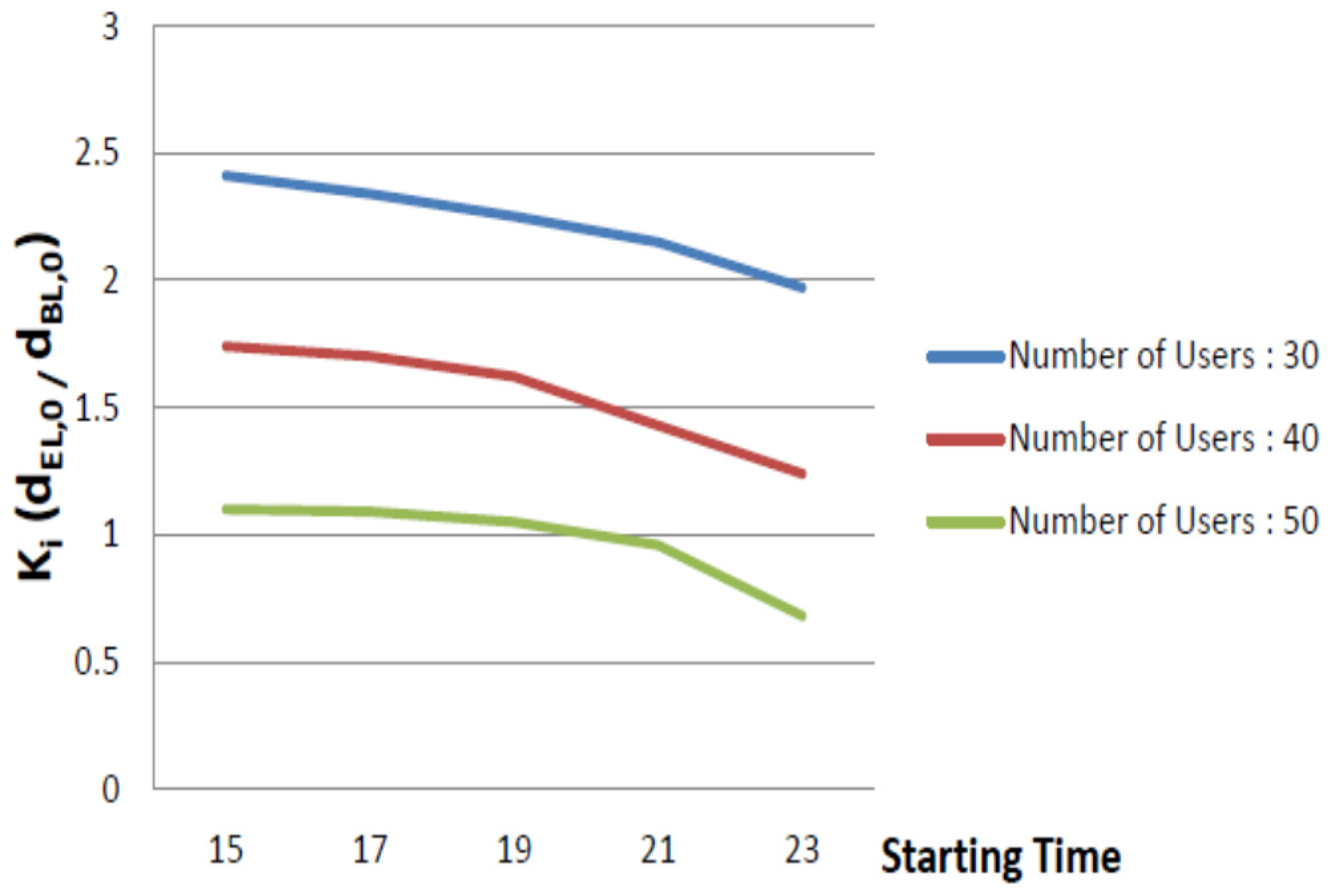
As shown in Figure 5 and Figure 6, let $K_i$ be a constant. When the starting time is approaching the actual TTT, the shorter $t_r$ can be used for transmissions and the value of $d_{BL,0}$ decreases accordingly. While the starting time is after 71 (Figure 4) or after 21 (Figure 5), $d_{BL,0}$ increases slightly and approaches a constant. This is because there is a shorter pre-scheduling time for transmissions after 71 (Figure 5) or after 21 (Figure 6), we need to assign a higher $d_{BL,0}$ for maintaining high QoS for streaming video. Furthermore, because of limitative pre-scheduling time, a greater number of users leads to higher $d_{BL,0}$ compared to a smaller number of users. On the other hand, high velocity causes a severe decrease of $d_{BL,0}$ because of a shorter pre-scheduling time.

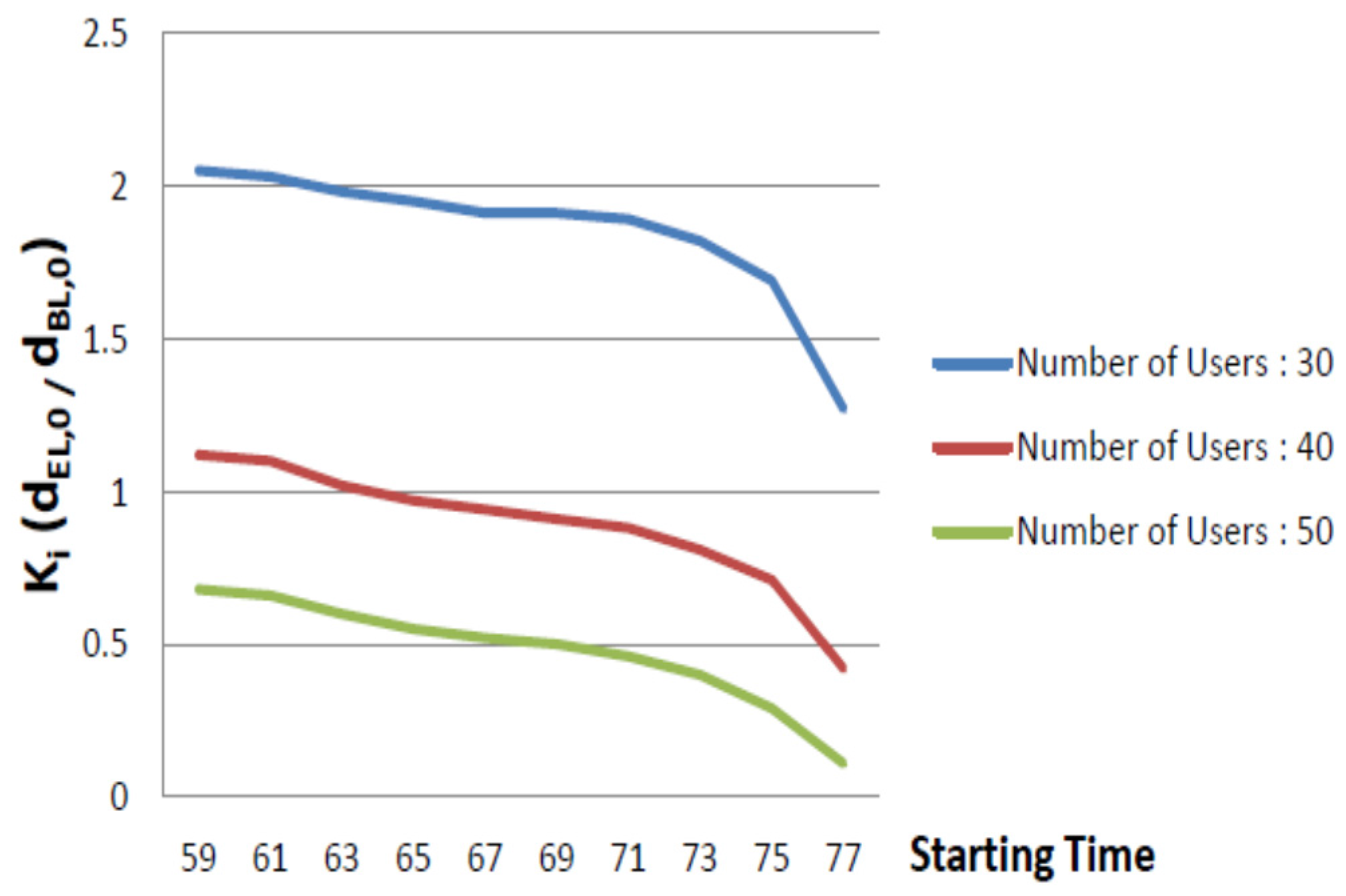
Because BL has higher priority for high QoS for video streaming, while the starting time is after 75 s (Figure 7) and 21 s (Figure 8), we can see $K_i$ has a severe decent rate, especially at higher velocity. This indicates our mechanism can provide more BL to meet high QoS for streaming video.

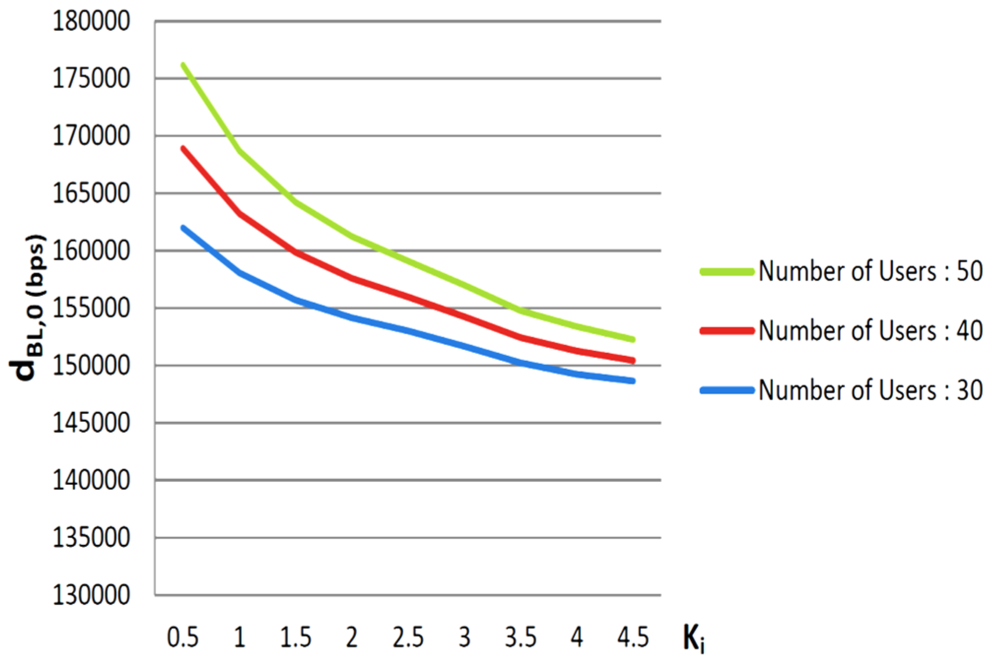
In the following, we set the length of pre-scheduling time $t_r$ to evaluate the relationship between $K_i$ and $d_{BL,0}$. Here, $K_i$ is a variable. In Figure 9 and Figure 10, a UE can dynamically adjust $K_i$ for desirable video quality according to SNR values. A higher $K_i$ indicates that $d_{BL,0}$ has a lower proportion of transmission frames. While the UE requires better video quality with more data of enhanced layers transmitted, $K_i$ can be set to a higher value. On the contrary, for a low SNR situation, $K_i$ can be set to a lower value to maintain high QoS for video streaming.

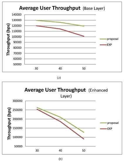
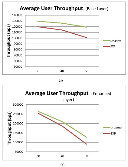
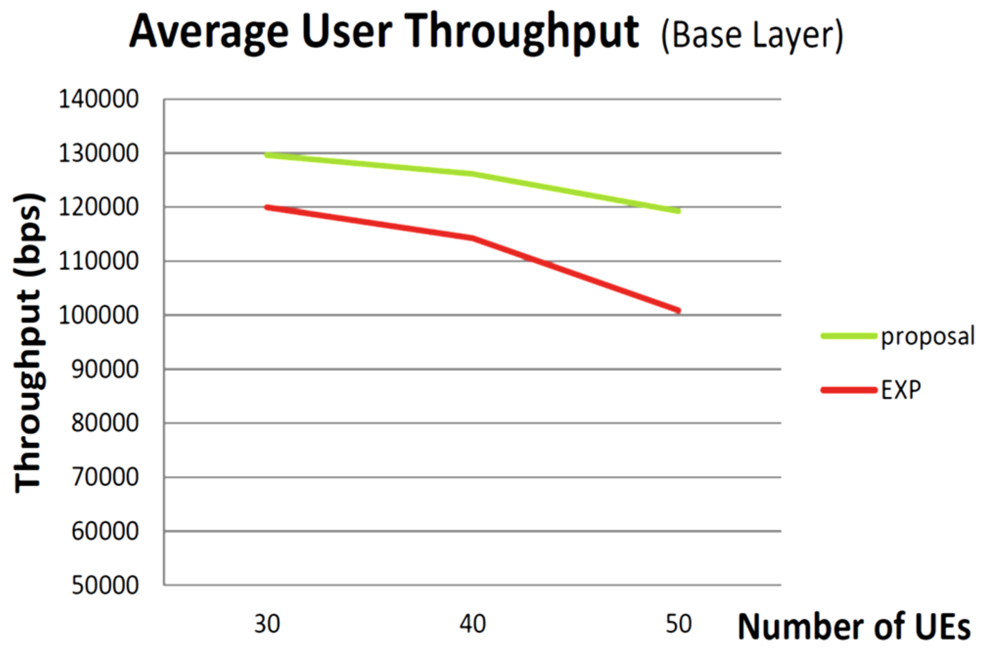
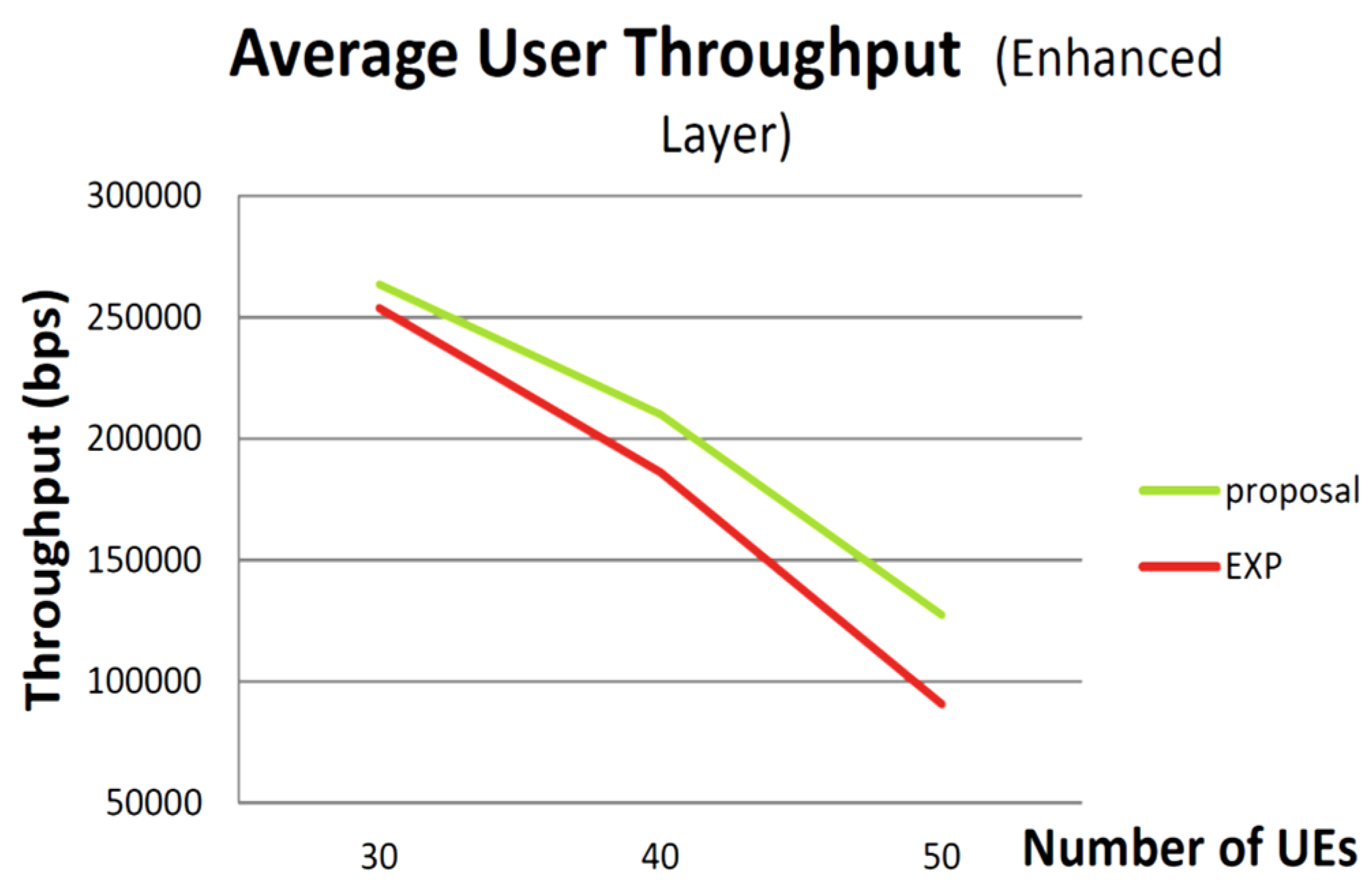
As shown in Figure 11 and Figure 12, our proposed mechanism achieves a higher throughput compared to the EXP/PF scheme. This is because BL has higher priority for transmission in our proposed mechanism. Furthermore, we combined the pre-scheduling mechanism with a prediction of TTT for packet transmissions. Note that BL is essential to video decoding, but the EXP/PF only fairly schedules BL and ELs transmissions.

4. Conclusions

In this paper, a pre-scheduling mechanism is proposed for real-time video delivery over LTE. We can adjust the data transmission rate before handover between BL and EL for high QoS for video streaming under the disconnection period by utilizing the handover prediction. The practical results show higher throughputs compared to the EXP/PF scheme.

References

- Chang, M.J.; Abichar, Z.; Hsu, C.Y. WiMAX or LTE: Who will lead the broadband mobile Internet? IT Prof. Mag. 2010, 12. [Google Scholar] [CrossRef]
- Dahlman, E.; Parkvall, S.; Skold, J.; Beming, P. 3G Evolution: HSPA and LTE for Mobile Broadband; Academic press: Burlington, MA, USA, 2010. [Google Scholar]
- Kwan, R.; Leung, C.; Zhang, J. Downlink Resource Scheduling in an LTE System; INTECH Open Access Publisher: Rijeka, Croatia, 2010. [Google Scholar]
- Proebster, M.; Mueller, C.M.; Bakker, H. Adaptive Fairness Control for a Proportional Fair LTE Scheduler. In Proceedings of the IEEE 21st International Symposium on Personal Indoor and Mobile Radio Communications (PIMRC), Instanbul, Turkey, 26–30 September 2010; pp. 1504–1509.
- Andrews, M.; Kumaran, K.; Ramanan, K.; Stolyar, A.; Whiting, P.; Vijayakumar, R. Providing quality of service over a shared wireless link. IEEE Commun. Mag. 2001, 39, 150–154. [Google Scholar] [CrossRef]
- Rhee, J.H.; Holtzman, J.M.; Kim, D.K. Scheduling of Real/Non-Real Time Services: Adaptive EXP/PF Algorithm. In Proceedings of the 57th IEEE Semiannual on Vehicular Technology Conference, Jeju, Korea, 22–25 April 2003; pp. 462–466.
- Ramli, H.A.M.; Basukala, R.; Sandrasegaran, K.; Patachaianand, R. Performance of Well Known Packet Scheduling Algorithms in the Downlink 3GPP LTE System. In Proceedings of the IEEE Malaysia International Conference on Communications (MICC), Kuala Lumpur, Malaysia, 15–17 December 2009; pp. 815–820.
- Afrin, N.; Brown, J.; Khan, J.Y. An Adaptive Buffer Based Semi-persistent Scheduling Scheme for Machine-to-Machine Communications over LTE. In Proceedings of the IEEE Eighth International Conference on Next Generation Mobile Apps, Services and Technologies (NGMAST), Oxford, UK, 10–12 September 2014; pp. 260–265.
- Patra, A.; Pauli, V.; Lang, Y. Packet Scheduling for Real-Time Communication over LTE Systems. In Proceedings of the IEEE Wireless Days (WD), Valencia, Spain, 13–15 November 2013; pp. 1–6.
- Piro, G.; Grieco, L.A.; Boggia, G.; Fortuna, R.; Camarda, P. Two-level downlink scheduling for real-time multimedia services in LTE networks. IEEE Trans. Multimed. 2011, 13, 1052–1065. [Google Scholar] [CrossRef]
- Xenakis, D.; Passas, N.; Merakos, L.; Verikoukis, C. ARCHON: An ANDSF-Assisted Energy-Efficient Vertical Handover Decision Algorithm for the Heterogeneous IEEE 802.11/LTE-Advanced Network. In Proceedings of the IEEE International Conference on Communications (ICC), Sydney, Australia, 10–14 June 2014; pp. 3166–3171.
- Xenakis, D.; Passas, N.; Verikoukis, C. A Novel Handover Decision Policy for Reducing Power Transmissions in the Two-Tier LTE Network. In Proceedings of the IEEE International Conference on the Communications (ICC), Ottawa, ON, Canada, 10–15 June 2012; pp. 1352–1356.
- Xenakis, D.; Passas, N.; Merakos, L.; Verikoukis, C. Mobility management for femtocells in LTE-advanced: Key aspects and survey of handover decision algorithms. IEEE Commun. Surv. Tutor. 2014, 16, 64–91. [Google Scholar] [CrossRef]
- Xenakis, D.; Passas, N.; Gregorio, L.D.; Verikoukis, C. A Context-Aware Vertical Handover Framework towards Energy-Efficiency. In Proceedings of the IEEE 73rd Vehicular Technology Conference (VTC Spring), Yokohama, Japan, 15–18 May 2011; pp. 1–5.
- Xenakis, D.; Passas, N.; Merakos, L.; Verikoukis, C. Energy-Efficient and Interference-Aware Handover Decision for the LTE-Advanced Femtocell Network. In Proceedings of the IEEE International Conference on Communications (ICC), Budapest, Hungary, 9–13 June 2013; pp. 2464–2468.
- Mesodiakaki, A.; Adelantado, F.; Alonso, L.; Verikoukis, C. Energy-efficient user association in cognitive heterogeneous networks. IEEE Commun. Mag. 2014, 52, 22–29. [Google Scholar] [CrossRef]
- LTE Simulator. Available online: http://telematics.poliba.it/LTE-Sim (accessed on 12 January 2015).
- Video Trace Library. Available online: http://trace.eas.asu.edu/ (accessed on 15 February 2015).
Figure 1.
Exponential smoothing (α = 0.2).
Figure 2.
Prediction for (a) time-to-trigger (TTT) of handover and (b) amount of data transmitted before handover.
Figure 3.
The data rate of (a) BL and (b) EL under degrading RSRP.
Figure 4.
The prediction of time-to-trigger (TTT) of handover. (a) User equipments (UEs) velocity = 30 km/h and (b) UE velocity = 120 km/h.
Figure 5.
Starting time for pre-scheduling vs. (UE velocity = 30 km/h, actual TTT = 79.924 s).
Figure 6.
Starting time for pre-scheduling vs. (UE velocity = 120 km/h, actual TTT = 25.981 s).
Figure 7.
The decent rate vs. starting time (UE velocity = 30 km/h).
Figure 8.
The decent rate vs. starting time (UE velocity = 120 km/h).
Figure 9.
The decent rate vs . (UE velocity = 30 km/h, = 20.924 s).
Figure 10.
The decent rate vs. (UE velocity = 120 km/h, = 8.981 s).
Figure 11.
Average user throughput (UE velocity = 30 km/h).
Figure 12.
Average user throughput (UE velocity = 120 km/h).