Blockwise Frequency Domain Active Noise Controller Over Distributed Networks

Abstract

This work presents a practical active noise control system composed of distributed and collaborative acoustic nodes. To this end, experimental tests have been carried out in a listening room with acoustic nodes equipped with loudspeakers and microphones. The communication among the nodes is simulated by software. We have considered a distributed algorithm based on the Filtered-x Least Mean Square (FxLMS) method that introduces collaboration between nodes following an incremental strategy. For improving the processing efficiency in practical scenarios where data acquisition systems work by blocks of samples, the frequency-domain partitioned block technique has been used. Implementation aspects such as computational complexity, processing time of the network and convergence of the algorithm have been analyzed. Experimental results show that, without constraints in the network communications, the proposed distributed algorithm achieves the same performance as the centralized version. The performance of the proposed algorithm over a network with a given communication delay is also included.

1. Introduction

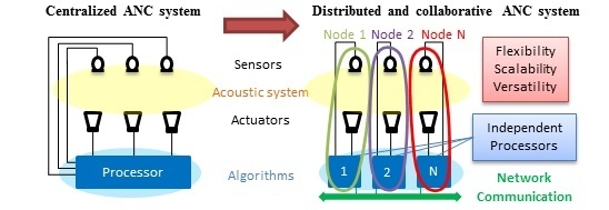
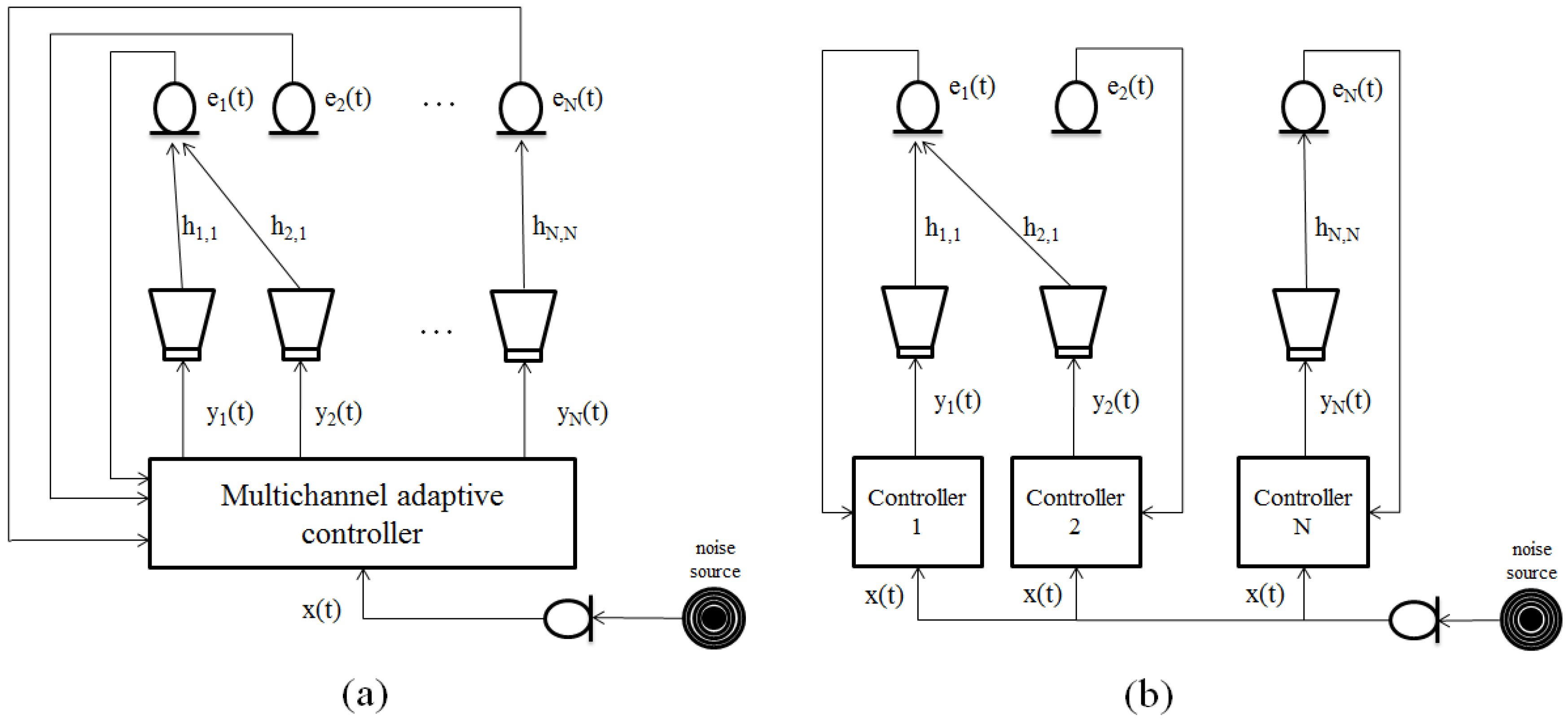
Active Noise Control (ANC) systems try to cancel, or at least minimize, some undesired noise by generating some sound signals specifically designed to cancel the first [1]. The global noise reduction is virtually impossible in an entire enclosure. Alternatively, we can attempt to control the noise field within a certain area to create local zones of quiet [2]. In particular, the system is intended to reduce the disturbance signal, called primary noise, at specific spatial points monitored by microphones, called error sensors. Generally speaking, the use of a large number of microphones strategically located produces larger zones of quiet. Similarly, multiple transducers are commonly used to improve the system performance, resulting in a multichannel ANC system. Typically, multichannel ANC systems use a single centralized processor managed by a control algorithm that has access to all the signals involved in the system. However, distributed systems offer a good solution to satisfy both high computational requirements and multiple signals capture, management and generation. Distributed systems are characterized by their flexibility, versatility and scalability. Flexibility allows the system to select the suitable strategy depending on the objective application. In addition, they have the versatility to adapt quickly and easily to different situations. Moreover, these systems can increase the number of controllers without redesigning the system. Therefore, a distributed system can be understood as a set of centralized systems that distribute the computational burden as well as the acquisition and signal generation to reach a common target. For example, a multichannel centralized controller can be distributed into several single-channel controllers (see Figure 1). In both systems, the error signals $e_k\left(t\right)$ are the signals recorded at the N microphones, the anti-noise signals $y_j\left(t\right)$ are the filter output signals reproduced by the N loudspeakers, the acoustic channels $h_{j,k}$ are the impulse responses between the jth loudspeaker and the kth microphone, and the reference signal $x\left(t\right)$ is the noise signal recorded at the reference sensor used by the adaptive controller to design the output signals $y_j\left(t\right)$ (where $k=1,2,\dots ,N$ and $j=1,2,\dots ,N$).

While centralized systems work with all the signals generated by the loudspeakers and captured by the microphones, distributed systems employ independent processors which control a subset of loudspeakers from the signals picked up by a subset of microphones. The concept of distributed ANC systems for sound control applications was first introduced in [3], which considers processors that work independently and do not interchange local information. Thus, the computational burden is distributed among the processors and, in the case that there was no acoustic interaction among loudspeakers and microphones, it is possible to reach the centralized cancelation solution. As Figure 1b shows and it is stated in [3], each error signal $e_k\left(t\right)$ is used only for its corresponding controller, and the reference signal $x\left(t\right)$ is common to all of them. Therefore, the use of a network that allows communication among the controllers would be beneficial for the distributed ANC system to achieve results equivalent to those of the centralized method. Recently, the miniaturization of electronic components is enabling a low-cost implementation of many types of electronic devices with a high performance as well. These devices are usually equipped with sensors and actuators, and they also contain increasingly powerful and efficient processors with communication capability. Moreover, despite their small size, they allow for a great autonomy as a result of the low power requirements. In the last decade, the cooperation and communications among these kind of devices to perform a specific task through the so-called Wireless Sensor Networks (WSN) has been addressed [4]. Such networks have many advantages and applications compared to the wired networks [5,6] such as scalability and low computational cost. For the purpose of monitoring and transmission of multimedia content, Wireless Multimedia Sensor Networks (WMSN) [7] are available, which require increased computational cost, synchronization, data transmission and energy consumption because of certain characteristics of the multimedia signals [8]. A subclass of WMSN are the Wireless Acoustic Sensor Networks (WASN) [9,10]. WASNs are a popular and efficient solution for different applications in multiple acoustic areas, such as environmental audio monitoring, binaural hearing aids, audio surveillance [11,12,13] as well as industrial monitoring and control [10]. WASNs offer many possibilities for developing new applications and strategies for audio processing due to the expansion of the area of interest and the low power, low cost and small size of the sensors [14]. These networks are usually composed of wireless devices, called nodes, randomly distributed in the environment and formed by a single microphone plus a processing unit with communication capability [15]. These passive nodes are dedicated to estimate parameters or signals common to all of them [16] or to a particular node [17]. However, for sound field control applications, such as ANC, elements or devices capable of measuring and generating signals are necessary. Furthermore, the network should focus on the estimate of the signals that will feed the loudspeakers in order to control and modify the sound field. Therefore, it is necessary to redefine the concept of acoustic node in order to use it in ANC applications. Thus, we define acoustic nodes as devices capable of obtaining information from one or more microphones and capable of generating signals via one or more loudspeakers. Moreover, every node has the ability to individually process signals as well as to interchange the necessary information with the other nodes using a suitable communication network. Therefore, a distributed network use a set of nodes, placed strategically to reach a common objective. An output signal at each node is generated as a result of processing the signal captured by the node as well as the information received from other nodes, when there exists communication among the nodes. Every node processes signals independently and all the nodes are relevant for the proper performance of the global system. It should be noted that the selection of the network topology will affect how data is processed by each node. Some common topology architectures are mesh, star, tree and ring topologies [18]. The proper election of the topology depends on the communication constraints dictated by the network such as the amount and frequency of the transmitted data, transmission distance, battery life of the node, etc. Note that, in real-time applications, some of these topologies introduce delays that could seriously affect the system performance [10]. Therefore, the use of synchronization mechanisms among nodes is necessary. Consequently, our target is to take advantage of the benefits of wireless acoustic sensor networks to implement active noise control systems in real environments. This work deals with the practical implementation of a distributed and collaborative active noise controller. To our knowledge, no other system of this type has been already reported.

The paper is organized as follows: in Section 2, we present a distributed solution that minimizes the power of the sum of the measured signals at the sensors’ locations over an Acoustic Sensor Network (ASN) without communication constraints and justifies the requirement of the distributed processing and the block-data processing in the frequency domain. In Section 3, the prototype description is given. The experimental results to compare the performance of both the distributed solution proposed and the centralized algorithm are shown in Section 4, including a discussion considering communication constraints. Finally, Section 5 outlines the main conclusions of the present work.

Notation: For the sake of clarity, the following notation has been used throughout this work: boldface lower-case denote vectors and matrices that contain information of signals in the time-domain (e.g., $\mathbf{e}$) and boldface upper-case letters denote vectors and matrices that contain information of the Fast Fourier Transform (FFT) of the previous signals (e.g., $\mathbf{E}$).

2. Collaborative Distributed Algorithm for an N-Nodes ASN Based on an Incremental Strategy

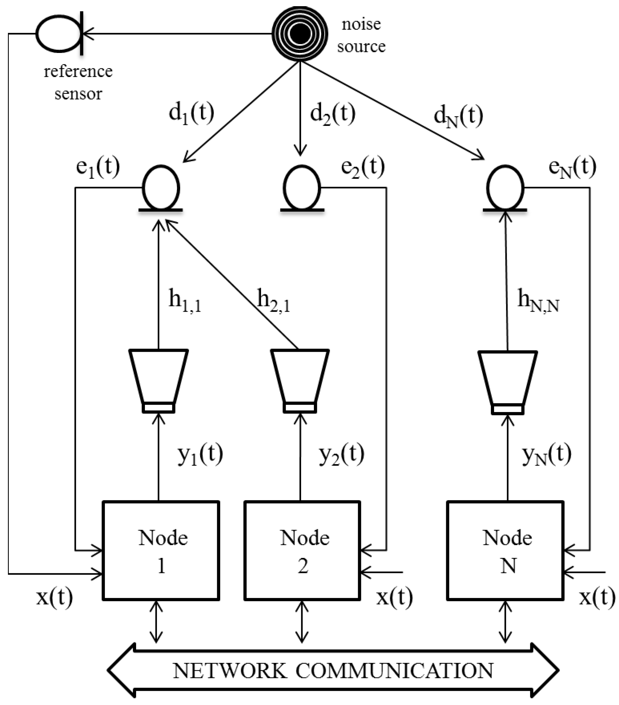
Consider a network of N nodes that supports an ANC system composed by N sensors and N actuators, as shown in Figure 2. For the sake of simplicity, we consider one disturbance noise and a distributed network of single-channel acoustic nodes in a homogeneous network. This implies that all the nodes have the same computation and communication capabilities, execute the same algorithm and are composed of a single sensor and a single actuator. The signals recorded at the sensors are called error signals and denoted by $e_k\left(t\right)$ (where $k=1,2,\dots ,N$), the actuators emit the filter output signals $y_j\left(t\right)$ (where $j=1,2,\dots ,N$), the acoustic channel impulse response between actuator j and sensor k is estimated as ${\mathbf{s}}_{jk}$, which is defined as the Finite Impulse Response (FIR) filter that models the estimation of the real acoustic channel ${\mathbf{h}}_{jk}$. In feedforward systems, the reference signal $x\left(t\right)$, is captured by a reference sensor employed to detect the acoustic noise far away from the area of interest. There exits only one noise source and all the nodes share the same reference signal $x\left(t\right)$. We aim at canceling the acoustic noise signal in the sensors location, $d_k\left(t\right)$, designing an adaptive filter ${\mathbf{w}}_k\left(t\right)$ at every node. Assuming that ${\mathbf{w}}_k\left(t\right)$ varies slowly, it can be written:

$$\mathbf{e}\left(t\right)=\mathbf{d}\left(t\right)+{\mathbf{w}}^T\left(t\right){\mathbf{x}}_f\left(t\right),$$

(1)

where the vectors $\mathbf{e}\left(t\right)={[e_1\left(t\right)e_2\left(t\right)\cdots e_N\left(t\right)]}^T$ and $\mathbf{d}\left(t\right)={[d_1\left(t\right)d_2\left(t\right)\cdots d_N\left(t\right)]}^T$ contain the error signals and desired signals, respectively, of the N nodes of the network, vector $\mathbf{w}\left(t\right)={[{\mathbf{w}}_1\left(t\right){\mathbf{w}}_2\left(t\right)\cdots {\mathbf{w}}_N\left(t\right)]}^T$ of size $LN\times 1$, concatenates the N adaptive filters ${\mathbf{w}}_k\left(t\right)$ that contain the L filter coefficients of the kth node at the time instant t. Matrix ${\mathbf{x}}_f\left(t\right)=[{\mathbf{x}}_{f,1}\left(t\right){\mathbf{x}}_{f,2}\left(t\right)\cdots {\mathbf{x}}_{f,N}\left(t\right)]$ is the concatenation of N vectors of size $LN\times 1$ defined as ${\mathbf{x}}_{f,k}\left(t\right)={[x_{f,1k}\left(t\right)x_{f,2k}\left(t\right)\cdots x_{f,Nk}\left(t\right)]}^T$ that contain the last L samples of the reference signal $x\left(t\right)$ filtered through the acoustic channel ${\mathbf{h}}_{jk}$ that links the actuator at the jth node with the sensor at the kth node. The objective is to estimate the coefficients vector $\mathbf{w}\left(t\right)$ that minimizes a cost function $J\left(t\right)$ that depends on the error signals $e_k\left(t\right)$. To do this, we use a gradient-descent method to estimate the coefficients in an iterative manner,

$$\mathbf{w}\left(t\right)=\mathbf{w}(t-1)-\mu {\nabla }_{\mathbf{w}}E\left\{J\left(t\right)\right\},$$

(2)

where μ is the step-size parameter, $E\{.\}$ is the expectation operator and ${\nabla }_{\mathbf{w}}=[{\nabla }_{{\mathbf{w}}_0}{\nabla }_{{\mathbf{w}}_1}\cdots {\nabla }_{{\mathbf{w}}_N}]$ being ${\nabla }_{{\mathbf{w}}_k}$ the gradient operator defined as the partial derivatives with respect to the coefficients vector $\mathbf{w}\left(t\right)$. The cost function is approximated by its instantaneous value by using the Least Mean Square (LMS) method [19], (${\nabla }_{\mathbf{w}}E\left\{J\left(t\right)\right\}\approx {\nabla }_{\mathbf{w}}\left(J\left(t\right)\right)$). Moreover and as stated in [20], we consider the sum of the power of the N instantaneous error signals as cost function,

$$J\left(t\right)=\sum _{k=1}^N{e}_k^2\left(t\right)=\mathbf{e}\left(t\right){\mathbf{e}}^T\left(t\right).$$

(3)

From Equation (3) and applying the gradient operator in Equation (1), we obtain

$$\mathbf{w}\left(t\right)=\mathbf{w}(t-1)-\mu {\mathbf{x}}_f\left(t\right)\mathbf{e}\left(t\right),$$

(4)

that can be rewritten as

$$\mathbf{w}\left(t\right)=\mathbf{w}(t-1)-\mu \sum _{k=1}^N{\mathbf{x}}_{f,k}\left(t\right)e_k\left(t\right).$$

(5)

Note that the computation of ${\mathbf{x}}_{f,k}\left(t\right)$ involves the real acoustic path ${\mathbf{h}}_{jk}$ which, in practical environments, can be estimated as ${\mathbf{s}}_{jk}$. Thus, the vector of size $LN\times 1$ that contains the last L samples of reference signal $x\left(t\right)$ filtered through ${\mathbf{s}}_{jk}$ is named as ${\mathbf{v}}_k\left(t\right)$ and substituting in Equation (5) leads to

$$\mathbf{w}\left(t\right)=\mathbf{w}(t-1)-\mu \sum _{k=1}^N{\mathbf{v}}_k\left(t\right)e_k\left(t\right).$$

(6)

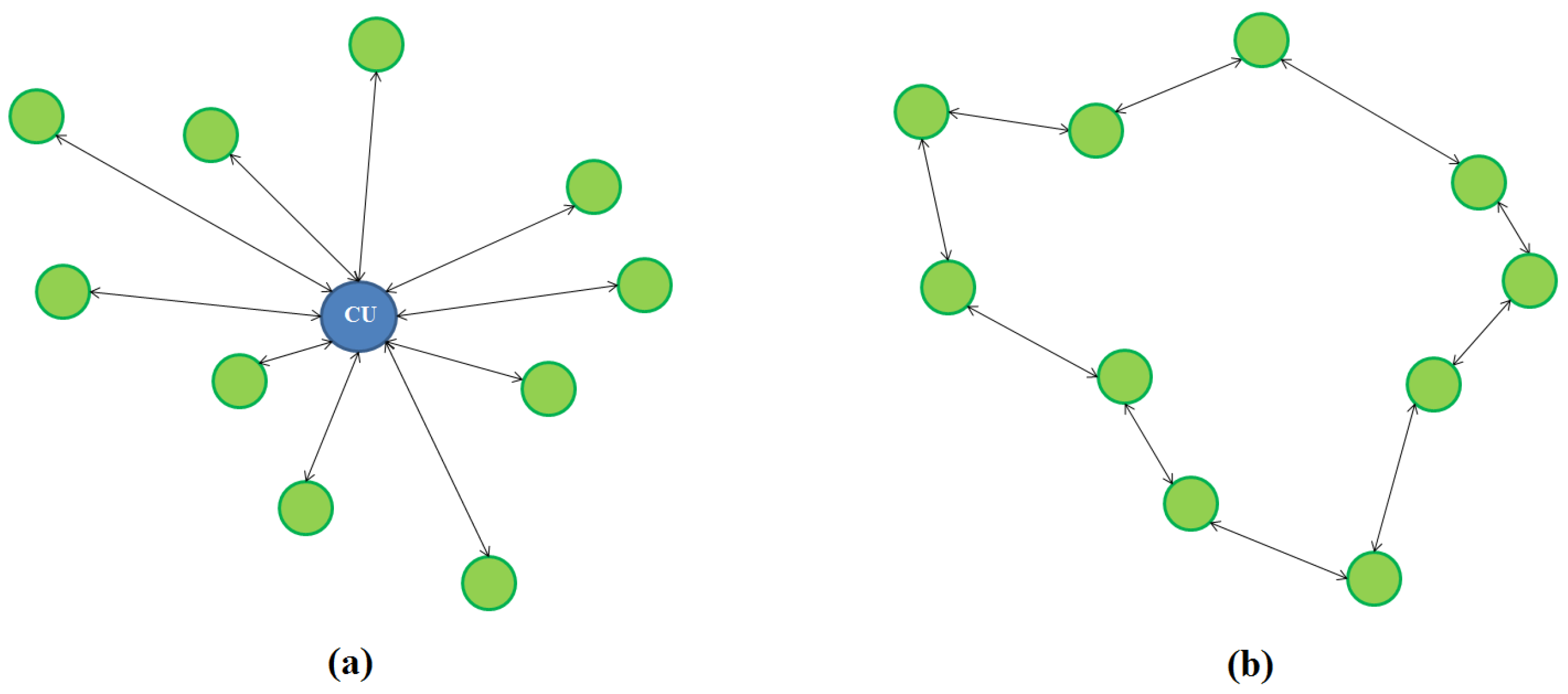
It can be seen in Equation (6) that all the error signals are necessary to calculate the coefficients of each filter, so that a central unit that receives and transmits all the information through the network is required (see Figure 3a). The problem is that, if the number of nodes increases or if multichannel nodes are used, it is not straightforward to transmit information between the central unit and each node due to an increase in the bandwidth required for communication. Moreover, any failure in the central unit will cause no information to be processed. Therefore, a distributed network (see Figure 3b) with the computational burden shared among the nodes becomes necessary to solve these problems. Since the number of signals processed at every node is low, this type of processing provides a more efficient computational performance. In addition, depending on the strategy used to exchange information among the nodes, the bandwidth in data transmission can be reduced. It should be noted that a distributed ASN in the context of this paper means that, not only are the nodes physically distributed in the area of interest, but also the processing (or computation) is divided among the nodes. Previous works [16,21] showed that the implementation of the LMS algorithm over distributed networks using collaborative strategies achieves good results. However, those works do not consider acoustic nodes that acoustically interact with the environment both controlling and modifying it, as it was introduced in [20]. A distributed ANC system based on the Multiple Error Filtered-x Least Mean Square (MEFxLMS) algorithm [20] and using incremental communication strategies with sample-by-sample data acquisition was presented in [22].

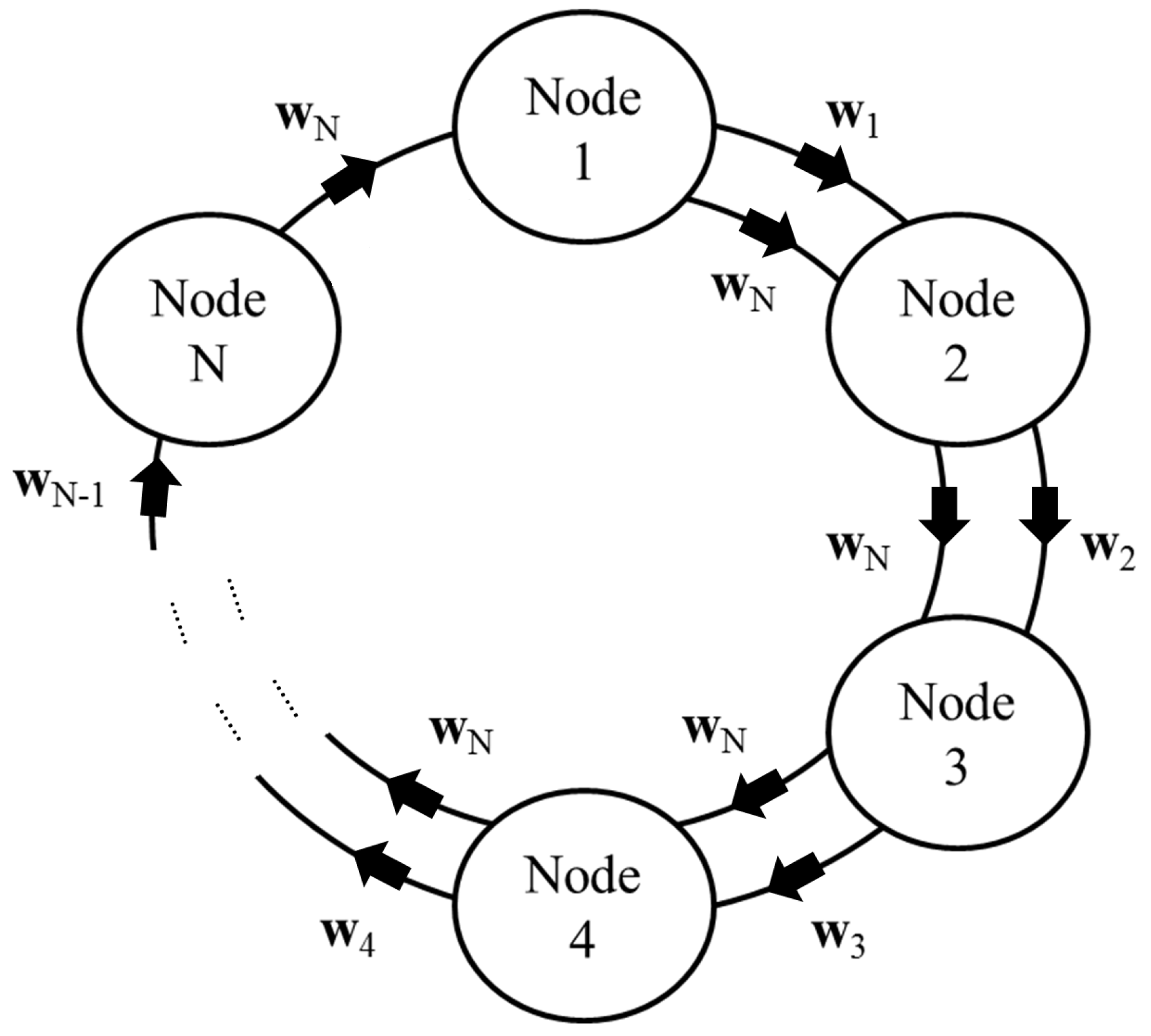
In the case of a ring network based on an incremental strategy, the coefficients of the adaptive filters are calculated by distributing the calculation among different nodes by transmitting information to an adjacent node in a consecutive order. Thus, every node can calculate a portion of the sum of the filter updating equation and supply to the next node the partial result to update the coefficients with its respective information. If this step is performed with an incremental strategy, the last node will have the complete updated coefficients. Finally, these coefficients are disseminated to the rest of the nodes to allow the system to generate the appropriate cancelation signals before the next iteration begins. This means $2(N-1)$ interchanges of the filter coefficients among the nodes (see Figure 4). Every kth node can share information with its adjacent $k+1$th node. Each node should calculate the adaptive filters of all the nodes of the network so, in a network of N nodes, the network state would be defined by N adaptive filters one of each node. If we define the global state of the network $\mathbf{w}\left(t\right)$ as the adaptive filter coefficients of each node of the network at the time instant t and considering ${\mathbf{w}}^k\left(t\right)$ a local version of $\mathbf{w}\left(t\right)$ at the kth node, Equation (6) may be written as:

$${\mathbf{w}}^k\left(t\right)={\mathbf{w}}^{k-1}\left(t\right)-\mu {\mathbf{v}}_k\left(t\right)e_k\left(t\right).$$

(7)

Equation (7) is the updating rule of the state of the kth node by using an iterative algorithm that minimizes Equation (3). Moreover, note that ${\mathbf{w}}^0\left(t\right)={\mathbf{w}}^N(t-1)=\mathbf{w}(t-1)$.

However, in real-time applications, the obtained equations have to be considered using block processing in the frequency domain in order to ensure a more efficient computational performance. The reason is because most common audio cards work with block data buffers. Moreover, hardware platforms that work with blocks of samples such as Digital Signal Processors (DSPs) or Graphics Processing Units (GPUs), use libraries of frequency-domain operations for a more efficient processing [23]. Furthermore, if the adaptive filters and the estimated secondary paths are longer than the sample block, they have to be split up into partitions [24]. For all these reasons, we consider the Frequency-domain Partitioned Block technique for the adaptive filtering operation [25,26] based on the conventional filtered-x scheme (FPBFxLMS). Notation in

Table 1. Notation of the description of the FPBFxLMS algorithm.

B	Block size
L	Length of the adaptive filters
M	Length of the Finite Impulse Response (FIR) filters that model the estimated secondary paths
F	$L/B$, number of partitions of the adaptive filters
P	$M/B$, Number of partitions of the estimated secondary paths
n	index that denotes block iteration
$f,p$	super-indexes that denote partition number.
${\mathbf{s}}_{jk}$	M-length estimation of the acoustic path that links the actuator at the jth node with the sensor at the kth node.
${\mathbf{S}}_{jk}^p$	Fast Fourier Transform (FFT) of size $2B$ of the pth partition of the acoustic path $s_{jk}$.

will be used to describe the following equations. Samples are processed by blocks of size B. L is the length of the adaptive filters, and M is the length of the FIR filters that model the estimated secondary path. F and P are the number of partitions of both the adaptive filters and the estimated secondary paths, respectively. Furthermore, the index n between brackets denotes block iteration and the super-indexes f and p denotes the number of the partition.

The vector ${\mathbf{x}}_B\left[n\right]={[x\left(Bn\right)x(Bn-1)\cdots x(Bn-B+1)]}^T$ contains the last B samples of $x\left(t\right)$ at discrete time instant t=$Bn$, and the error vector ${\mathbf{e}}_{k,B}\left[n\right]$ contains the last block of size B of the error signal $e_k\left(t\right)$ in the node k at discrete time instant t=$Bn$, ${\mathbf{e}}_{k,B}\left[n\right]={[e_k\left(Bn\right)e_k(Bn-1)\cdots e_k(Bn-B+1)]}^T$. The vector $\mathbf{X}\left[n\right]$ contain the FFT of size $2B$ of the vector ${\mathbf{x}}_B\left[n\right]$ in the actual block iteration and the same vector in the previous block iteration, $\mathbf{X}\left[n\right]=\mathrm{FFT}\left[{\mathbf{x}}_B[n-1]{\mathbf{x}}_B\left[n\right]\right]$ and the vector ${\mathbf{E}}_k\left[n\right]$ is the FFT of size $2B$ of the error vector ${\mathbf{e}}_{k,B}\left[n\right]$ preceded by a vector of zeros of size B, ${\mathbf{0}}_B$. Note that we only consider the last B samples of the $2B$-Inverse Fast Fourier Transform (IFFT) operation, $\mathrm{IFFT}\left\{\mathbf{Y}\right[n\left]\right\}$, as the valid samples of the adaptive filter output ${\mathbf{y}}_B\left[n\right]$ since the first B samples suffer the effects of circular convolution due both to data management and the FFT sizes. Now, we define

$$\mathbf{W}\left[n\right]=\left[\begin{array}{c}{\mathbf{W}}_1\left[n\right],{\mathbf{W}}_2\left[n\right],\cdots ,{\mathbf{W}}_N\left[n\right],\end{array}\right]$$

(8)

being ${\mathbf{W}}_k\left[n\right]=\left[\begin{array}{c}{\mathbf{W}}_k^1\left[n\right],{\mathbf{W}}_k^2\left[n\right],\cdots ,{\mathbf{W}}_k^F\left[n\right]\end{array}\right]$ a matrix of size $[2B\times F]$ where ${\mathbf{W}}_k^f\left[n\right]$ contains the $2B$-FFT of the fth partition of the adaptive filter of the kth node. The N nodes collaborate with each other by updating their part of $\mathbf{W}\left[n\right]$ and transferring $\mathbf{W}\left[n\right]$ to the next node. Therefore, every node will use a local version of the global state of the network (denoted by ${\widehat{\mathbf{W}}}_k\left[n\right]$) at the kth node at the nth block iteration. Notice that only the F partitions of $2B$ coefficients of their adaptive filter are needed to generate the kth node output signal:

$${\mathbf{W}}_k[n-1]={\widehat{\mathbf{W}}}_N{[n-1]}_{(:,1+F(k-1):Fk)}.$$

(9)

Moreover, we define

$${\mathbf{V}}_k\left[n\right]=\left[\begin{array}{c}{\mathbf{V}}_{1k}\left[n\right],{\mathbf{V}}_{2k}\left[n\right],\cdots {\mathbf{V}}_{Nk}\left[n\right],\end{array}\right]$$

(10)

being ${\mathbf{V}}_{jk}\left[n\right]=\left[\begin{array}{c}{\mathbf{V}}_{jk}^1\left[n\right],{\mathbf{V}}_{jk}^2\left[n\right],\cdots ,{\mathbf{V}}_{jk}^F\left[n\right]\end{array}\right]$ a matrix of size $[2B\times F]$ where vector ${\mathbf{V}}_{jk}^f\left[n\right]$ contains the $2B$-FFT of the reference signal filtered with the fth partition of the estimated acoustic channel ${\mathbf{s}}_{jk}$. Each node estimates the coefficients of the rest of the nodes to achieve a global solution using the information of the previous node and the adaptation matrix calculated using the signals that each node own. Derived from the FPBFxLMS algorithm in [26], we can rewrite Equation (7) in the frequency domain with blocks of B samples. Thus, the update equation of the adaptive filter coefficients of the kth node at the nth block iteration is given by

$${\widehat{\mathbf{W}}}_k\left[n\right]={\widehat{\mathbf{W}}}_{k-1}\left[n\right]-\mu \mathrm{FFT}\left\{\left[{\left[\mathrm{IFFT}\{{\underline{\mathbf{E}}}_k\left[n\right]\circ {{\mathbf{V}}_k\left[n\right]}^{*}\}\right]}_{[1:B,:]}{\mathbf{0}}_{[B\times FN]}\right]\right\},$$

(11)

where ${\underline{\mathbf{E}}}_k\left[n\right]$ is the multiplication of vector ${\mathbf{E}}_k\left[n\right]$ by ${\mathbf{1}}_{[1\times FN]}$, a row vector of ones of size $FN$. Constant μ is the step-size parameter and the operators FFT and IFFT perform the direct and inverse fast Fourier transform of size $2B$ of each column of the matrixes involved. ∘ denotes the element-wise product of two matrices, * denotes complex conjugation and ${\mathbf{0}}_{[B\times FN]}$ is a matrix of zeros of size $[B\times FN]$. Note that we only consider the first B samples of the $2B$-IFFT operation. Once all the nodes have finished the filter coefficient updates, the global vector ${\widehat{\mathbf{W}}}_N\left[n\right]$ is disseminated to the rest of the nodes for the (n+1)th iteration. Note that in (11), ${\widehat{\mathbf{W}}}_0\left[n\right]={\widehat{\mathbf{W}}}_N[n-1]$, as we stated in Equation (7). Algorithm 1 illustrates the summary of the algorithm instructions, which are executed per block iteration at each node.

Algorithm 1 Distributed FPBP x LMS Algorithm for N-nodes ASN

1: $\mathbf{for}\mathbf{all}node1\le k\le N\mathbf{do}$

2:   ${\mathbf{W}}_k[n-1]={\widehat{\mathbf{W}}}_k{[n-1]}_{(:,1+F(k-1):Fk)}$

3:   ${\displaystyle {\mathbf{Y}}_k\left[n\right]=\sum _{f=1}^F{\mathbf{W}}_k[n-1]\circ \mathbf{X}[n-f+1]}$

4:   $\mathbf{for}\mathbf{all}1\le j\le N\mathbf{do}$

5:         ${\displaystyle {\mathbf{V}}_{jk}\left[n\right]=\sum _{p=1}^P{\mathbf{S}}_{jk}^p\circ \mathbf{X}[n-p+1]}$

6:   $\mathbf{end}\mathbf{for}$

7:   ${\mathbf{V}}_k\left[n\right]=[{\mathbf{V}}_{1k}\left[n\right],{\mathbf{V}}_{2k}\left[n\right],\cdots {\mathbf{V}}_{Nk}\left[n\right]]$

9:   ${\mathbf{E}}_k\left[n\right]=\mathrm{FFT}\left\{\left[{\mathbf{0}}_B{\mathbf{e}}_B\left[n\right]\right]\right\}$

10:   ${\underline{\mathbf{E}}}_k\left[n\right]={\mathbf{E}}_k\left[n\right]·{\mathbf{1}}_{[1\times FN]}$

11:   ${\widehat{\mathbf{W}}}_k[n]={\widehat{\mathbf{W}}}_{k-1}[n]-\mu \mathrm{FFT}\{[{[\mathrm{IFFT}\{{\underline{\mathbf{E}}}_k[n]\circ {{\mathbf{V}}_k[n]}^{*}\}]}_{[1:B,:]}{\mathbf{0}}_{[B\times FN]}]\}$

12: $\mathbf{end}\mathbf{for}$

13: $\mathbf{for}\mathbf{all}node0\le k\le N\mathbf{do}$

14:   ${\widehat{\mathbf{W}}}_k\left[n\right]={\widehat{\mathbf{W}}}_N\left[n\right]$

15: $\mathbf{end}\mathbf{for}$

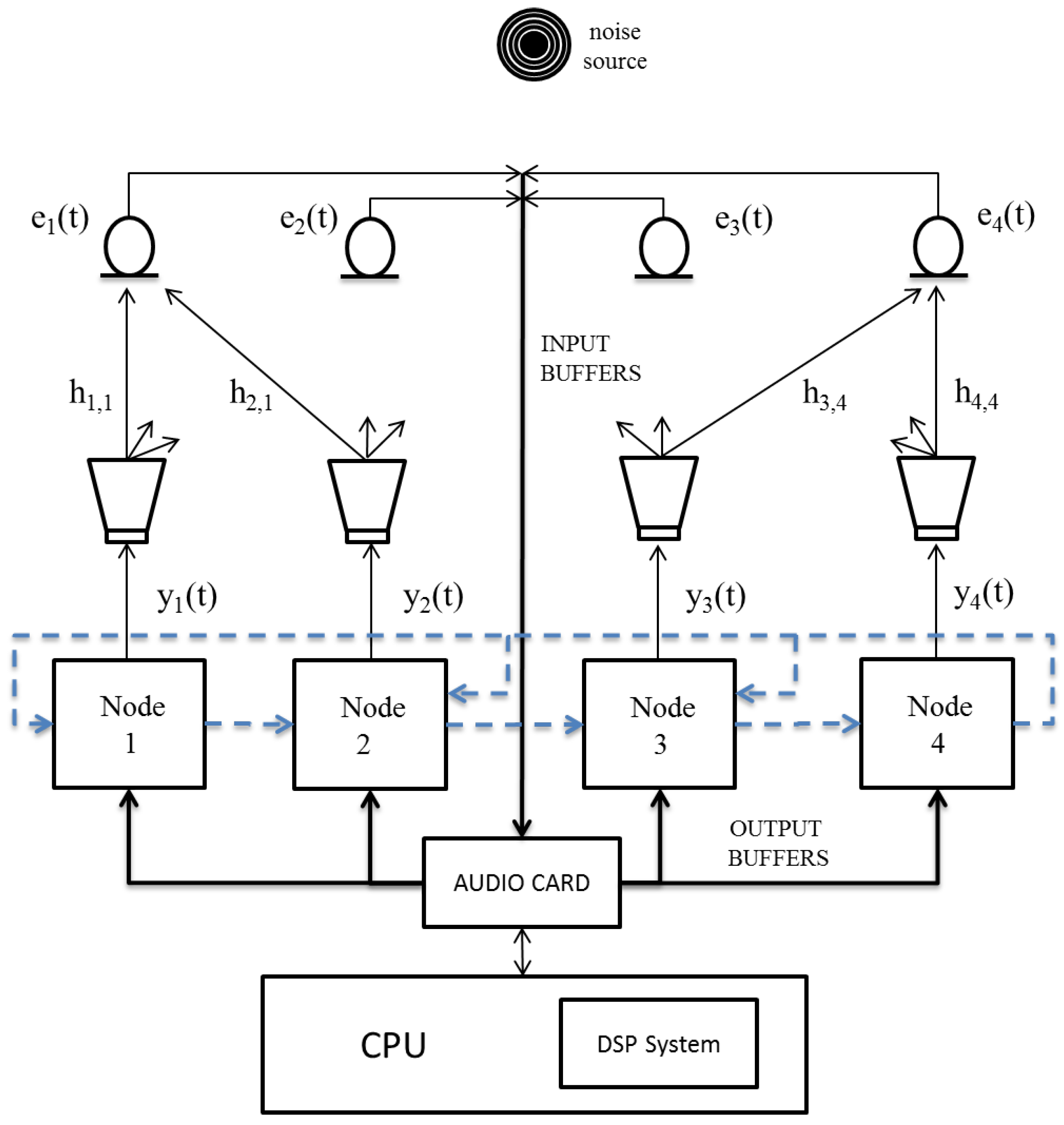
3. Prototype Description

The distributed ANC prototype is depicted in Figure 5. The addition of the recent DSP System Toolbox [27] in the computing environment MATLAB^® provides multichannel real-time audio recording, processing and reproduction at low latency. Audio objects based on Object Oriented Programming (OOP) have been optimized for iterative computations that process large streams of audio data. Moreover, Audio Stream Input/Output (ASIO) drivers [28] have been incorporated to this software providing a low-latency and high fidelity interface between MATLAB^® and audio card. The hardware implementation is composed by a CPU (Intel Core i7 3.07 GHz) and an audio card (MOTU 24 I/O). The communication between both components is performed by ASIO drivers and it is controlled by using the MATLAB^® System objects provided by the DSP System Toolbox of MATLAB^® software. The audio card stores the input data from the sensor of each node in buffers of size B and send them to the CPU through the ASIO drivers. The CPU, with MATLAB^® support, executes the audio processing, saves the output data in buffers and sends them back to the audio card through the ASIO drivers, to be reproduced by the loudspeaker of each node.

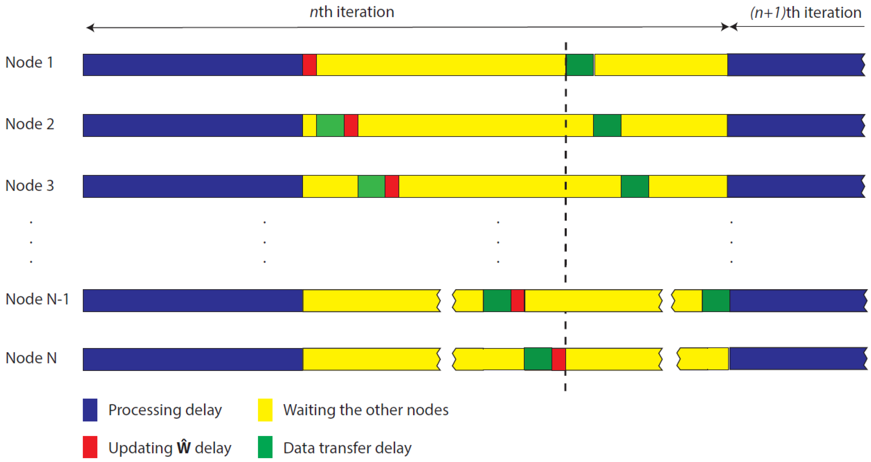
The selection of the block size B in the audio card is critical to determine the latency of the algorithm. The latency is the sum of the time spent on storing data in the input buffers, on processing these data and on sending them to the output buffers as well. A real-time application must satisfy that the time spent to fill up the input buffers (buffering time) was higher than the time spent in data processing (processing time). The buffering time is defined as $B/fs$, $fs$ being the sampling rate. In a centralized ANC system, the processing time is the time that the algorithm takes to process data. However, in a distributed ANC system, it also includes the time in updating its own global state of the network ($\widehat{\mathbf{W}}$) and in delivering this information among the nodes. As we consider an incremental network composed of N nodes, every node must transfer $2L\times N$ coefficients (size of $\widehat{\mathbf{W}}$) to the following node $2(N-1)$ times in each block iteration (see Figure 4). Therefore, the processing time of the whole network at each block iteration (algorithm processing time + N times the updating time of $\widehat{\mathbf{W}}$ + $2(N-1)$ times the transmission time of $\widehat{\mathbf{W}}$) has to be less than the buffering time (see Figure 6). As an example, a transfer rate at least of 16.5 megabytes per second (MBps) would be necessary with an incremental network composed of four nodes, a general filter length of 4096 taps and single-precision floating-point data format. Therefore, using a standard Ethernet network of 1 Gbps (≈ 125 MBps), we would have enough rate capacity to perform the required data transfer among the nodes. It should be noted that, if the processing time of the network increases due to the addition of more nodes, the buffering time must be increased in order to satisfy the real-time condition. Hence, if we assume a fixed sampling rate, the block size B must be increased.

Another important aspect that should be guaranteed is the causality of the system. The algorithm has to satisfy that the sum of the buffering delay and the maximum delay of the acoustic paths that join the actuators with the error sensors should be less than or equal to the minimum delay of the acoustic paths that join the noise source with the error sensors [29]. Causality constraint can be relaxed when a harmonic excitation is considered, but it is important in broadband noise control. As we perform an ANC system in a acoustic enclosure, where the wavelength is relatively low in comparison with the physical dimensions of the system, the causality condition is fulfilled by carefully choosing the distances between the noise source, actuators and error sensors. However, if this condition is not met, a decrease in buffering time is required. When these requirements are fulfilled and assuming a network of synchronized nodes, the proposed distributed algorithm can achieve the same performance as the centralized version.

The sampling rate of the audio card was fixed at $44.1$ kHz, the lowest possible rate, because of audio signals are typically sampled at that value (CD quality). The audio card offers different values of B between 16 and 2048 samples. Due to the real-time condition explained previously, we have selected $B=2048$ as a tradeoff between the processing time of the network and the buffering time.

It should be noted that the algorithms execute their processing in real time but, for simplicity, the communication network and the network distributed processing are emulated. All the nodes share the same central processing unit (CPU) but the implemented code allows a distributed and independent processing, simulating the processing carried out in a real distributed ASNs. Therefore, a basic networking hardware dedicated to the information exchange (a physical layer of the network) is not considered. The communication among the nodes is virtual, thanks to the code designed in MATLAB^® software.

4. Experimental Results

In this section, we show the experiments carried out to validate the performance of the distributed algorithm for unconstrained and constrained networks. For this purpose, in the first stage, we have evaluated and compared the convergence behavior, the noise reduction and the computational complexity of both distributed and centralized ANC systems in a ideal network. In the second stage, a performance analysis of the distributed algorithm over non-ideal networks has been carried out. 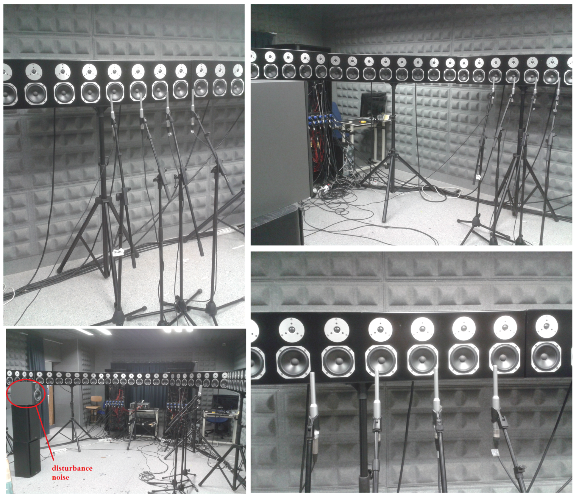The experiments have used the prototype described in Section 3 inside a listened room of $9.36$ meters long, $4.78$ meters wide and $2.63$ meters high, located at the Audio Processing Laboratory of the Polytechnic University of Valencia [30]. This room has an array of 96 loudspeakers mounted in an orthogonal structure. A photograph of the listening room and the different settings can be seen in Figure 7. For all the designed ASNs, the real acoustic responses between all the loudspeakers and all microphones are identified off-line using adaptive methods and modeled as FIR filters of $M=4096$ coefficients at a sampling rate of $44.1$ kHz. We have considered a zero-mean Gaussian white noise with unit variance as disturbance noise, which is emitted by a loudspeaker located in front of the loudspeakers and microphones that compose the ASN, as it is shown in Figure 7. Since practical ANC systems are suitable to cancel low-frequency noise signals, we have considered a broadband white noise limited to 200 Hz. Furthermore, we have considered a block size of $B=2048$ and an adaptive filter length of $L=4096$ coefficients. A constant step size parameter of $\mu =8\times {10}^{-5}$, as the highest value that ensures the stability of the algorithms, has been used.

The configuration of the ASN is depicted in Figure 5. Four nodes composed by one loudspeaker and one microphone each of them were considered. The loudspeakers were selected from the array with an equal separation of 20 cm between adjacent loudspeakers. The microphones were placed opposite to the loudspeakers and separated 40 cm away from them. The separation between the microphones was 20 cm. Future applications closely related to the tested distribution would be related to the creation of local quiet zones in enclosures using moderate size networks of sound nodes with likely acoustic interaction between at least a few of them—for example, a cabin of a public transport (train, plane, bus, etc.) where the separation between actuators and sensors would be similar than the detailed above. For the experimental tests, two different scenarios have been evaluated:

• ANC system over a four-node ideal network controlled by the FPBFxLMS distributed algorithm and its centralized version.
• ANC system over a four-node non-ideal network controlled by the FPBFxLMS distributed algorithm, comparing the results with the same algorithm but introducing constant delays in the data exchanges through the network. Now we assume that the nodes interchange information every Np block iterations, being p a constant positive integer and N the number of single-channel nodes. During the remainder Np-1 block iterations, we assume two cases. In case 1, the nodes just wait for the arrival of new network information trying to simulate a network with limited power, which saves as much energy as possible. In case 2, the nodes will use its local information to update their filter coefficients. Moreover, we assume that the diffusion of the global state of the network ${\widehat{\mathbf{W}}}_N\left[n\right]$ from the last node N to the rest of the nodes (see Figure 4) is not considered in this scenario.

In order to evaluate the performance of the different algorithms, we define the instantaneous Noise Reduction at node k, ${NR}_k\left(t\right)$, as the ratio in dB between the estimated error power with and without the application of the active noise controller:

$$N{R}_k\left(t\right)={10\times log}_{10}\left[\begin{array}{c}\frac{e_k^2\left(t\right)}{d_k^2\left(t\right)}\end{array}\right],$$

(12)

here $d_k^2\left(t\right)$ is the signal power picked up at the kth microphone when the ANC system is inactive and $e_k^2\left(t\right)$ is the error signal power measured at the kth microphone when the ANC system works. Moreover, these signals powers have been estimated using an exponential windowing from the instantaneous signals.

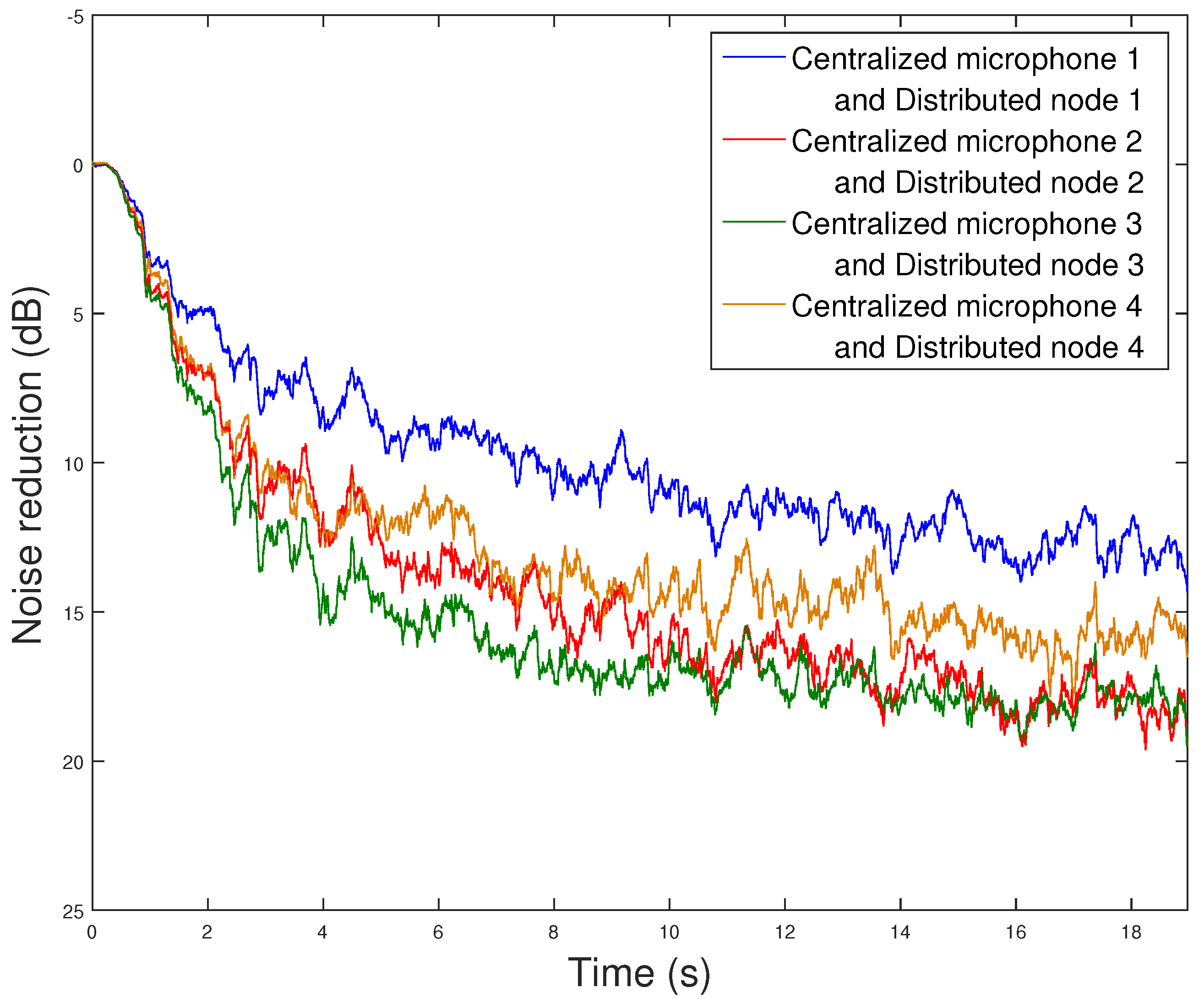
In the first scenario, we have evaluated the performance of both the distributed and the centralized FPBFxLMS algorithm in a network composed of four single-channel nodes with no communications constraints. Figure 8 shows the ${NR}_k\left(t\right)$ by using Equation (12) for both algorithms. As expected, the distributed implementation exhibits the same performance than the centralized implementation for the four nodes. Both algorithms show a robust and stable performance providing an attenuation up to 11 dB for the worst node and almost 20 dB for the best node.

Table 2. Total number of multiplications (MUX), additions (ADD) and Fast Fourier Transforms (FFTs) per blockwise iteration of the FPBFxLMS algorithm in both: (1) centralized and (2) distributed ANC systems. L: length of the adaptive filters; N: number of nodes.

	Operations	Generic	N = 1	N = 4	N = 8
	MUX	4 $LN$ + 4 $L{N}^2$	8 L	80 L	288 L
(1)	ADD	$LN$ + 3 $L{N}^2$	4 L	52 L	200 L
	FFTs	2 + 6 N	8	26	50
	MUX	2 L + 6 $LN$	8 L	26 L	50 L
(2)	ADD	L + 3 $LN$	4 L	13 L	25 L
	FFTs	4 + 4 N	8	20	36

compares the computational complexity in terms of multiplications, additions, and FFTs per iteration of the FPBFxLMS algorithm, implemented for a centralized and a distributed ANC systems. For the centralized implementation, we consider a multichannel ANC system with one disturbance noise and the same number of microphones and loudspeakers (1:N:N configuration). For the distributed implementation, we consider a network of N single-channel nodes. It is important to note that the complexity of the network as a whole is at least as high as the centralized algorithm. However, note that each node processes the algorithm simultaneously except the last addition of the global network state of the previous node (see line 11 in Algorithm 1). Therefore, in Table 2, we have only computed the operations of one single-channel node. Since we use a value of $M=L$, and $B=L/2$ (two partitions) the computational complexity only depends on L and N. First, the third column of Table 2 shows the computational complexity of both algorithms related to values of L and N. Then, this computational complexity is particularized for $N=1$, $N=4$ and $N=8$. As expected, when $N=1$, both implementations need the same number of operations. This is because both the centralized and the distributed ANC systems become a single-channel system. Moreover, for $N=4$, we compare the operations of a centralized ANC system with a 1:4:4 configuration (16 channels) with the operations of a single-channel node of a network of four nodes. Finally, the same is done for $N=8$. Results show that in a centralized ANC system, the computational complexity increases significatively with the number of channels. This fact represents a bottleneck in massive multichannel ANC systems. Otherwise, the increase of computational complexity in a distributed ANC system is not so significant.

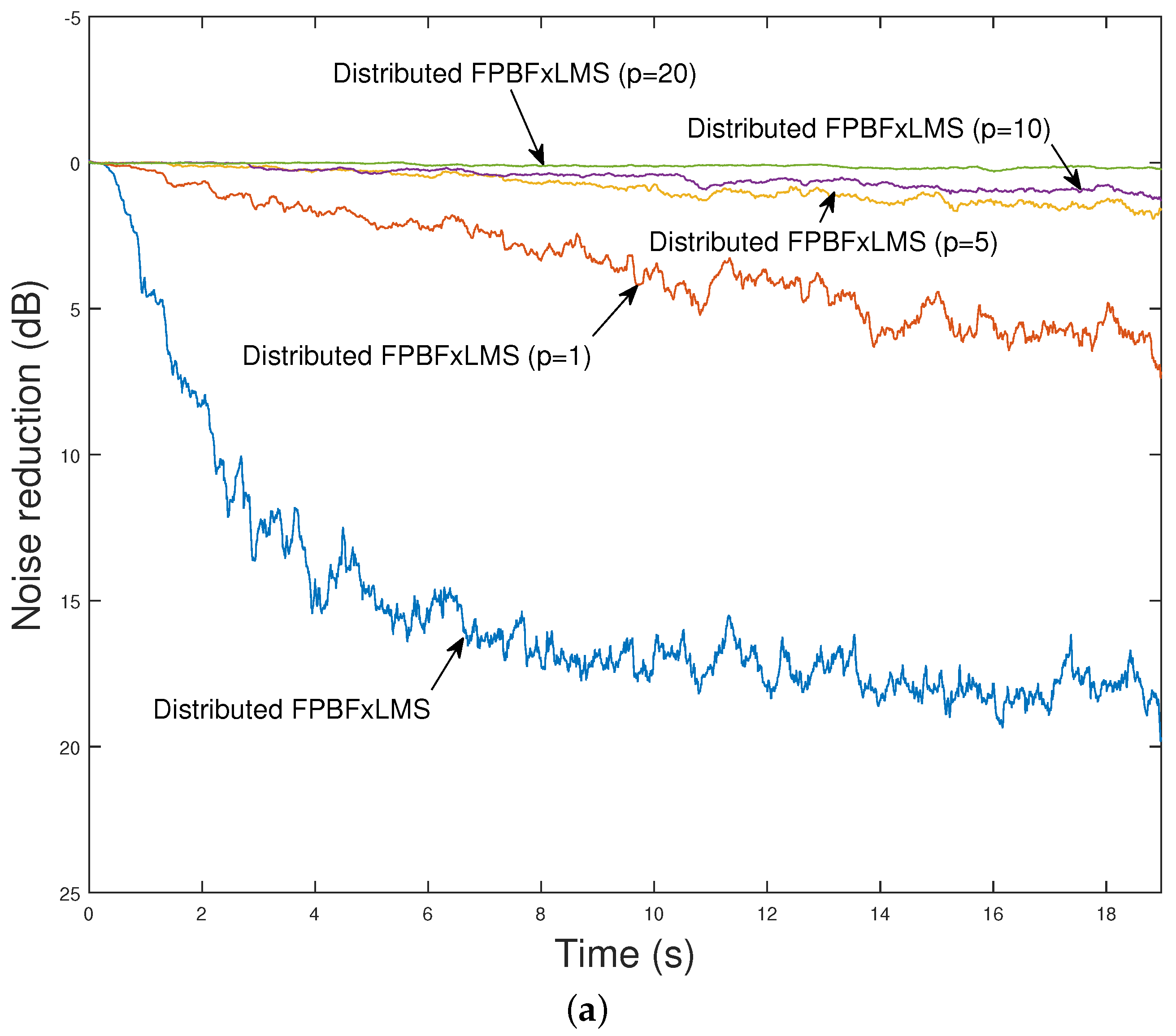
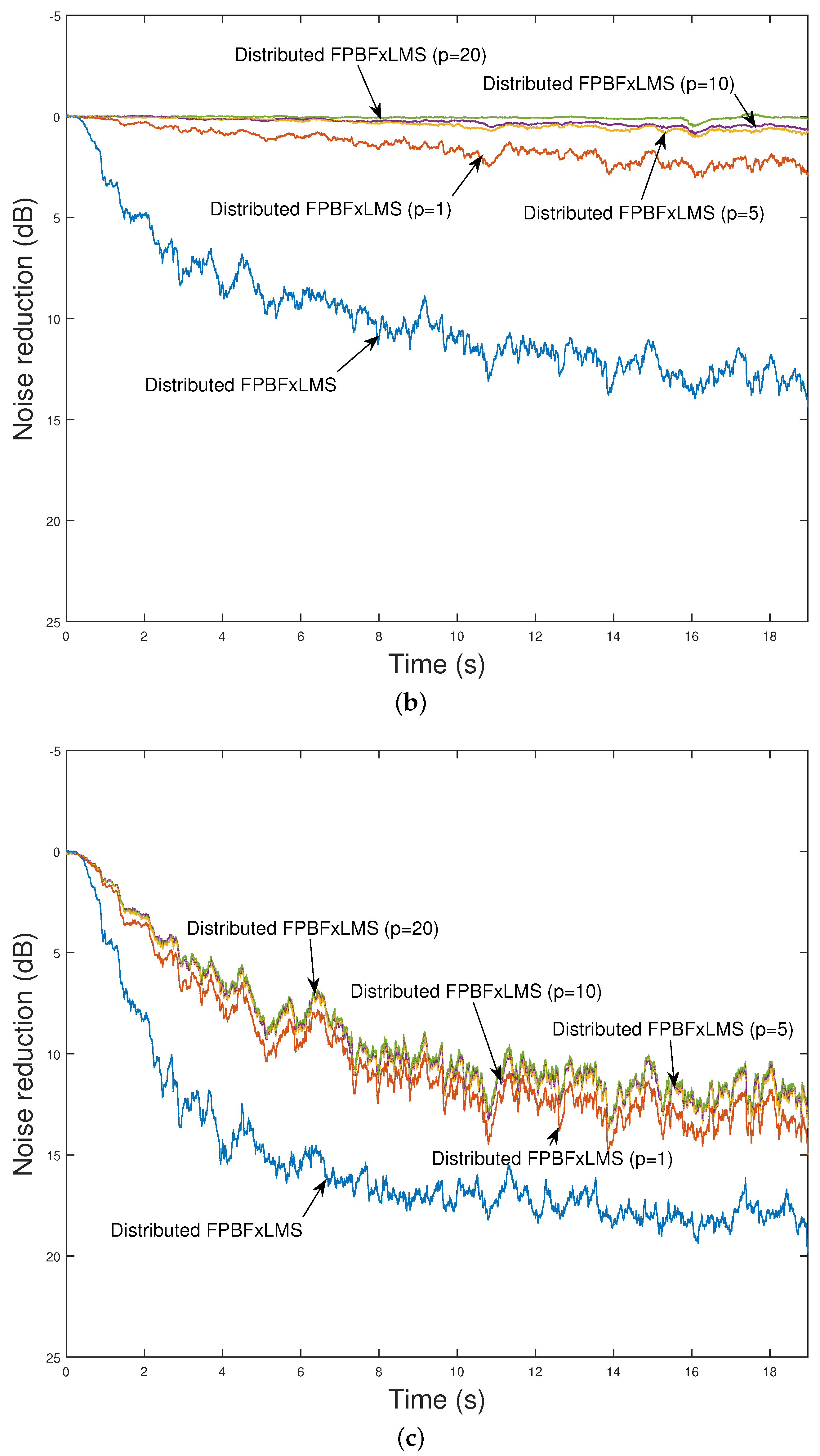
In the second scenario, the influence of a constant delay between information exchanges within a four-node network on the behavior of the distributed FPBFxLMS algorithm has been evaluated. The ${NR}_k\left(t\right)$ curves of the best node in the network with different delay values of p are presented in Figure 9a for case 1 and Figure 9c for case 2. In both cases, as p increases, the performance of the algorithm gets worse. However, when the nodes performs their local updating while waiting for the network information (case 2), the influence of the increased delay is lower than in case 1, obtaining an ${NR}_k\left(t\right)$ in all cases only 5 dB lower than the case of an ideal network. Similar results are obtained for the node with the worst performance. 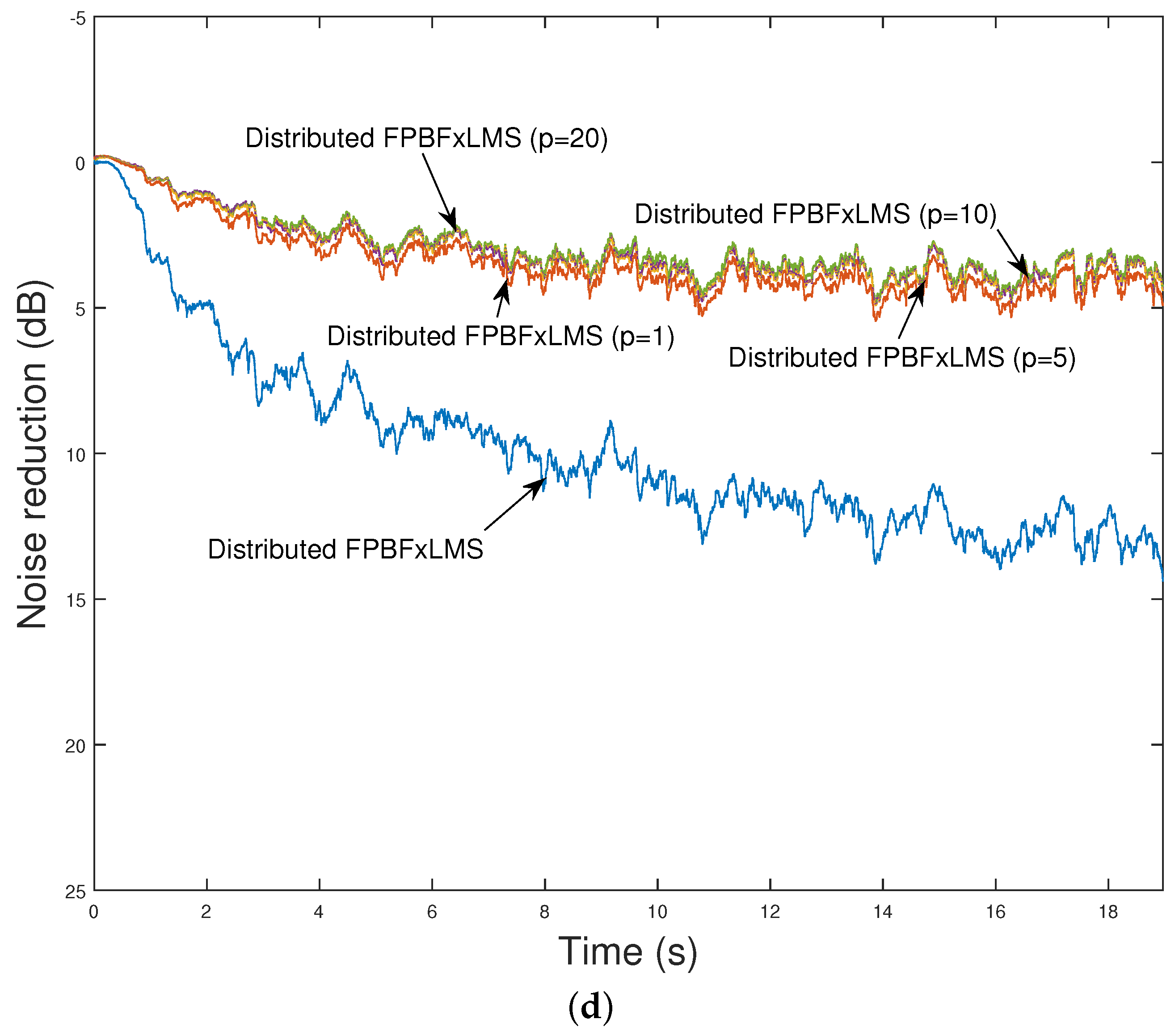Figure 9 shows the ${NR}_k\left(t\right)$ curves of the worst node in the network with different values of p, (b) for the case 1 and (d) for the case 2. Therefore, for networks with communication constraints, the behavior of the system can be improved if the nodes are allowed to update their filter coefficients while waiting for the network information. It is important to take into account that the final behavior of both cases depends on the degree of acoustic interaction between nodes, and, therefore, it should be studied in future works.

Finally, note that all the results accomplished in this work depend on particular settings, but their behavior can be easily extrapolated to other configurations.

5. Conclusions

In this paper, an experimental validation of an ANC system has developed over a network of distributed acoustic nodes using a collaborative incremental strategy. For this purpose, a distributed version of the FPBFxLMS algorithm has been introduced. In order to evaluate the performance of the proposed algorithms in a practical environment, we have implemented the adaptive control in a real-time audio toolbox provided by MATLAB^®. Results show that the distributed implementation of the algorithm exhibits the same performance as its centralized version when there are no communication constraints in the network.

Moreover, the computational complexity of the distributed algorithm has been studied and compared with the centralized version. Since each node of the distributed algorithm can perform almost all the operations simultaneously, the computational complexity is split among the nodes and the processing time of the algorithm is significantly reduced. However, when we consider the use of physical nodes in a real network, we will have to analyze some aspects with regards to the communication capabilities among the nodes in the network. In this sense, we can conclude that the distributed ANC system performs well if the network has enough bandwidth to transfer the network information without violating the real-time condition.

The performance of the proposed distributed FPBFxLMS algorithm in an ideal ASN and an ASN with a constant delay in the communications has been also shown. The behavior of the system worsens when delay increases, but, in this experiment, it shows an acceptable and stable performance despite data loss in the information exchange when the node uses its local information while waiting for network information. However, the influence of the degree of acoustic interaction between nodes on the network communication strategies must be considered in future works.