Sound Radiation of Aerodynamically Excited Flat Plates into Cavities

Abstract

Flow-induced vibrations and the sound radiation of flexible plate structures of different thickness mounted in a rigid plate are experimentally investigated. Therefore, flow properties and turbulent boundary layer parameters are determined through measurements with a hot-wire anemometer in an aeroacoustic wind tunnel. Furthermore, the excitation of the vibrating plate is examined by laser scanning vibrometry. To describe the sound radiation and the sound transmission of the flexible aluminium plates into cavities, a cuboid-shaped room with adjustable volume and 34 flush-mounted microphones is installed at the non flow-excited side of the aluminium plates. Results showed that the sound field inside the cavity is on the one hand dependent on the flow parameters and the plate thickness and on the other hand on the cavity volume which indirectly influences the level and the distribution of the sound pressure behind the flexible plate through different excited modes.

1. Introduction

There are noise sources everywhere in our environment, and these sounds are transferred in different ways to the human ear. The simplified generic model subject to this investigation reflects the type of sound excitation and transmission that occurs in numerous applications, e.g. in passenger vehicles, such as cars, buses, trains or planes. This undesirable sound is caused by excited flat structure elements. Today, people are constantly exposed to continuous noise which constitutes one of the most serious problems of our time [1]. Therefore, a growing need for personal acoustic shielding arises. The increasing travel time for great distances is indirectly leading to higher driving velocities to save time in turn. Thus, the flow noise develops to the dominating driving noise. In this context, there are numerous scientific studies discussing individual issues of the noise origination without considering the entire effect chain, starting with excitation, over the sound radiation und transmission to the sound detection.

Recent studies analyzed the flow-induced vibration of a plate with a crosswise prefixed obstacle plate and an additional external exciter with a varying frequency and amplitude [2]. External forces often have an effect on flow-excited plates. It turned out that both excitations are influencing the dynamics of the system. The frequencies of both test modes appear in the frequency spectrum at a low amplitude of the external harmonic excitation, whereas the external excitation in a coupled system is prevailing at a higher amplitude.

Concerning the sound radiation into a room, there were vibroacoustical analytical investigations on a model of a railway vehicle body [3]. The structure-induced noise radiation of flexible floor panels was analyzed and the natural frequencies and the sound pressure field inside the cavity were analytically determined. The result of the study is that significant resonance peaks arise from two concentrated forces on the plate if the dominant excitation frequency approaches the natural frequencies of the system. Moreover, the rise of the flow velocity led to an increase in the sound pressure inside the cavity. Regarding the spatial distribution of the sound pressure, it was found that the sound pressure above the excitation points takes remarkably higher values.

Numerous cases regarding the flow over different obstacles have already been investigated. Low importance has been attached to the sound radiation of a plate and the coupled distribution inside a cavity yet. However, two novel studies considering this subject were published this year. Shi et al. [4] focussed on the analytical modeling of a three-dimensional coupled acoustic system consisting of a cavity with a coupled flexible plate and a semi-infinite expanded field. The excitation of the system, including acoustic and structural-acoustic coupling, is generated inside the cavity by a point source. A solution method was found to predict the dynamic behavior of the entire system using Fourier series to express the sound pressure and the displacement of the plate. The results are validated through numerical simulations. This approach examined the issue which will be covered in detail in this paper, but only in an analytical way with an excitation in reverse direction without the influence of an external flow.

Ganji and Dowell [5] investigated the sound transmission into and radiation from a cavity through a flexible plate structure in a noisy/thermal environment in a supersonic flow. Using nonlinear models for the pre- and the postflutter regions, equations for the flexible panel, cavity acoustics and turbulent boundary layer are developed. Based on several approaches and theories, the resulting equations are solved numerically. The results for the postflutter domain are high sound pressure levels in the lower-frequency regions and a Helmholtz resonator condition with homogenous sound pressure distribution inside the cavity.

While there are numerical and analytical studies, there are hardly any experimental investigations. This paper provides correlations between the excitation, the sound radiation and the sound detection. In particular, the flow is characterized, the plate vibration analyzed and the measured sound inside the cavity is described.

The aim of this study is to understand the effects of different influences on the sound radiation and the sound transmission of flexible plate structures with different measuring configurations. The effect chain of a clearly defined excitation should be understood in small scale and hereinafter transferred to special application fields. Moreover, an additional flexible plate could be added and different damping and absorbing materials could be analyzed to reduce the sound radiation and transmission.

2. Theory

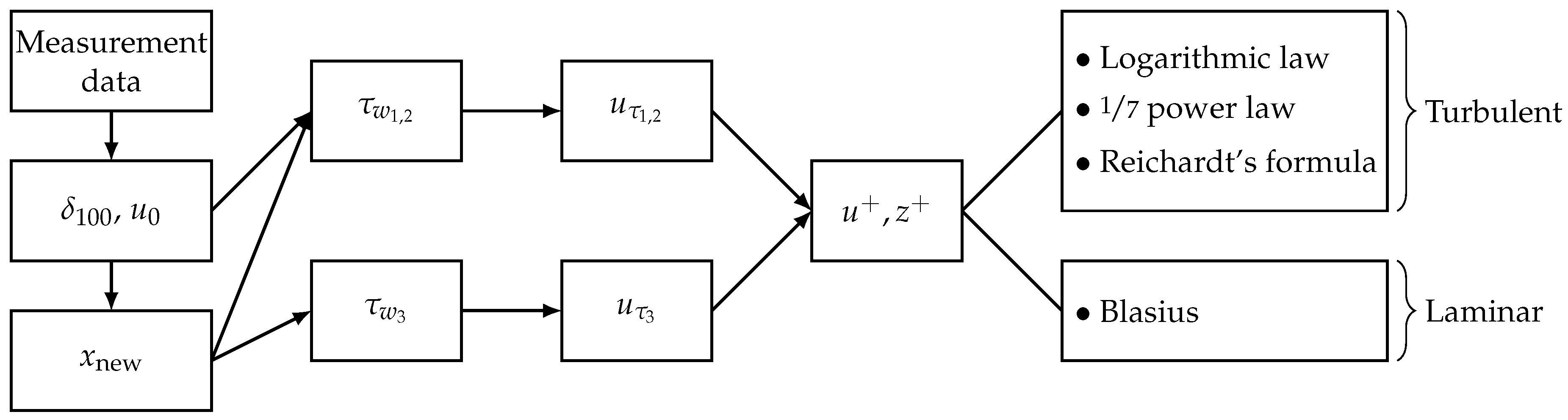
Before analyzing the sound radiation of the plate, a determination of the boundary layer parameters is required to achieve a starting position with well-defined initial and boundary conditions. For illustrative purposes, a scheme of the theoretical setup is depicted in Figure 1.

To specify whether the boundary layer is laminar or turbulent, an analytical calculation of the dimensionless velocity profiles is required. Therefore, different approximate solutions for the wall shear stress ${\tau }_w$ are examined in detail. The first one has resulted from empirical measurements of a pipe flow and can be transferred to smooth plate walls due to similarity. The analogous approach for a turbulent boundary layer [6,7]

$$\frac{u_{\infty }}{u_{\tau }}=8.75{\left(\frac{u_{\tau }\delta }{\nu }\right)}^{\frac{1}{7}}$$

(1)

is solved for the friction velocity with the main flow velocity $u_{\infty }$, the wall shear stress velocity $u_{\tau }$, the boundary layer thickness $\delta$ and the kinematic viscosity $\nu$. Using the following equation ${\tau }_w=\rho u_{\tau }^2$ with the density $\rho$ yields:

$${\tau }_{w_1}=0.0225·\rho u_{\infty }^2{\left(\frac{\nu }{u_{\infty }·\delta }\right)}^{\frac{1}{4}}$$

(2)

The boundary layer thickness $\delta$ of the turbulent flow as a function of the running length x is developed through substitution in conjunction with the $1/7$ power law, rearrangement and integration from 0 to x [6,8]:

$$\delta (x)=0.371·x·{{Re}_x}^{-\frac{1}{5}}.$$

(3)

with the Reynolds number based on the running length in flow direction ${Re}_x$. For Reynolds numbers ranging from $5\times {10}^5$ to ${10}^7$, the local friction coefficient for a turbulent flow over an isothermal plate is correlated by [9,10]:

$$C_{f,x}=0.0592·{{Re}_x}^{-\frac{1}{5}}$$

(4)

The friction coefficient as the dimensionless shear stress is defined as [9]:

$$C_{f,x}=\frac{{\tau }_w}{{\displaystyle \frac{\rho }{2}·{u_{\infty }}^2}}$$

(5)

Equalizing the two Equations (4) and (5) results in the following wall shear stress ${\tau }_{w_2}$ as second equation:

$${\tau }_{w_2}=0.0296·\rho u_{\infty }^2{{Re}_x}^{-\frac{1}{5}}$$

(6)

We tried to approach the velocity distribution in the boundary layer to the real course of the experimental measurement data. Indirect turbulence models are used as a basis of the direct velocity modeling:

• $\mathbf{1}/\mathbf{7}$ Power Law [6,9]

$$u(z)=u_{\infty }·{\left(\frac{z}{\delta (x)}\right)}^{\frac{1}{7}}$$

(7)

with the distance perpendicular to the plate z. The dimensionless velocity is calculated using the following equation ${\displaystyle u^{+}=\frac{u(z)}{u_{\tau }}}$ with ${\displaystyle u_{\tau }=\sqrt{\frac{{\tau }_w}{\rho }}}$.

• Logarithmic Law after Coles and Adapted by Golliard [11,12]

The dimensionless velocity which follows the outer-layer corrected logarithmic law after Coles is given by:

$$u^{+}=\frac{u(z-z_0)}{u_{\tau }}=\frac{1}{\kappa }ln\left({Re}_{\delta }\frac{u_{\tau }}{u_{\infty }}\xi \right)+B+\frac{\mathsf{\Pi }}{\kappa }\omega \left(\xi \right)(0\le (z-z_0)\le \delta )$$

(8)

This indirect turbulence model uses a Reynolds number which is based on the boundary layer thickness $\delta$:

$${Re}_{\delta }=\frac{u_{\infty }\delta }{\nu }$$

(9)

The dimensionless wall distance $\xi$ is defined as

$$\xi =\frac{z-z_0}{\delta },$$

(10)

with the position of the wall $z_0$. The von Kármán constant is $\kappa$ = 0.4 [11] and the boundary layer constant is $B=5.1$. Hinze [13] fitted the data analytically from an empirical table after Coles and derived the following relation for the wake-function:

$$\omega \left(\xi \right)=1-cos\left(\pi \xi \right)=2{sin}^2\left(\frac{\pi }{2}\frac{z}{\delta }\right)$$

(11)

The profile parameter $\mathsf{\Pi }$ is dependent on the pressure gradient and results in Equation (8) for $\xi =1$. At this point the velocity is $u_{\infty }$ and the z-coordinate corresponds to the boundary layer thickness $\delta$.

$$\mathsf{\Pi }=\frac{\kappa }{2}\frac{u_{\infty }}{u_{\tau }}-\frac{1}{2}ln\left({Re}_{\delta }\frac{u_{\tau }}{u_{\infty }}\right)-\frac{B\kappa }{2}$$

(12)

• Reichardt’s Formula [14]

$$u^{+}=\frac{1}{\kappa }ln\left(1+\kappa z^{+}\right)+7.8\left[1-{exp}^{-\frac{z^{+}}{11}}-\frac{z^{+}}{11}{exp}^{-0.33z^{+}}\right]$$

(13)

with the dimensionless wall distance ${\displaystyle z^{+}=\frac{z·u_{\tau }}{\nu }}$.

Regarding the laminar boundary layer, there is a solution in general form of the simplified approximated form of the boundary layer equations after Prandtl for the special case of a flat plate [9]. The appropriate derivation through a similarity clause was realized by Blasius [9]. In this case, another formula for the wall shear stress according to the laminar boundary layer is used:

$${\tau }_{w_3}=0.332·\rho u_{\infty }^2{{Re}_x}^{-\frac{1}{2}}$$

(14)

The running length x is defined so that it takes the value 0 at the front edge of the rigid plate, which is connected to the wind tunnel, and represents the x-position of the measured velocity profiles. This position is either directly or indirectly (by using the Reynolds number) required to calculate the wall shear stress. Moreover, this assumption states a boundary layer which is turbulent from the beginning and ’normally’ developing in x-direction. However, the transition from laminar to turbulent in this investigation is artificially created by a roughness trip located at the inner wall of the nozzle. Thus, the transition occurs in a certain distance, which is displaced in the downstream direction and not unambiguously determinable. Consequently, a new x-position is reverse calculated by rearranging Equation (3):

$$x_{\mathrm{new}}={\left(\frac{{\delta }_{100}·{u_{\infty }}^{\frac{1}{5}}}{0.371·{\nu }^{\frac{1}{5}}}\right)}^{\frac{5}{4}}$$

(15)

The boundary layer thickness ${\delta }_{100}$ and the velocity $u_0$ at the boundary layer border are directly estimated from the hot-wire measurements because usual definitions are not sufficient. For this case, it can not assumed that the boundary layer thickness is the position where $u_0$ takes a constant value of $0.99·u_{\infty }$. Therefore, the measurement data are fitted with a spline curve. To determine its gradient, a moving average with a window width of 50 samples is used due to the noise caused fluctuations of the flow velocity at the boundary layer border. At the beginning the gradient is high but it decreases constantly to almost zero. Below a gradient of 0.05, only minor velocity fluctuations occur which leads to a good approximation of the wall distance z for the boundary layer thickness ${\delta }_{100}$.

3. Materials and Methods

This section mentions all the measurement methods with its associated measuring setups and evaluation procedures.

3.1. Experimental Setup

The following subsections deal with the experimental setups that have been utilized to measure the fluid flow and the sound field.

3.1.1. Flow Field

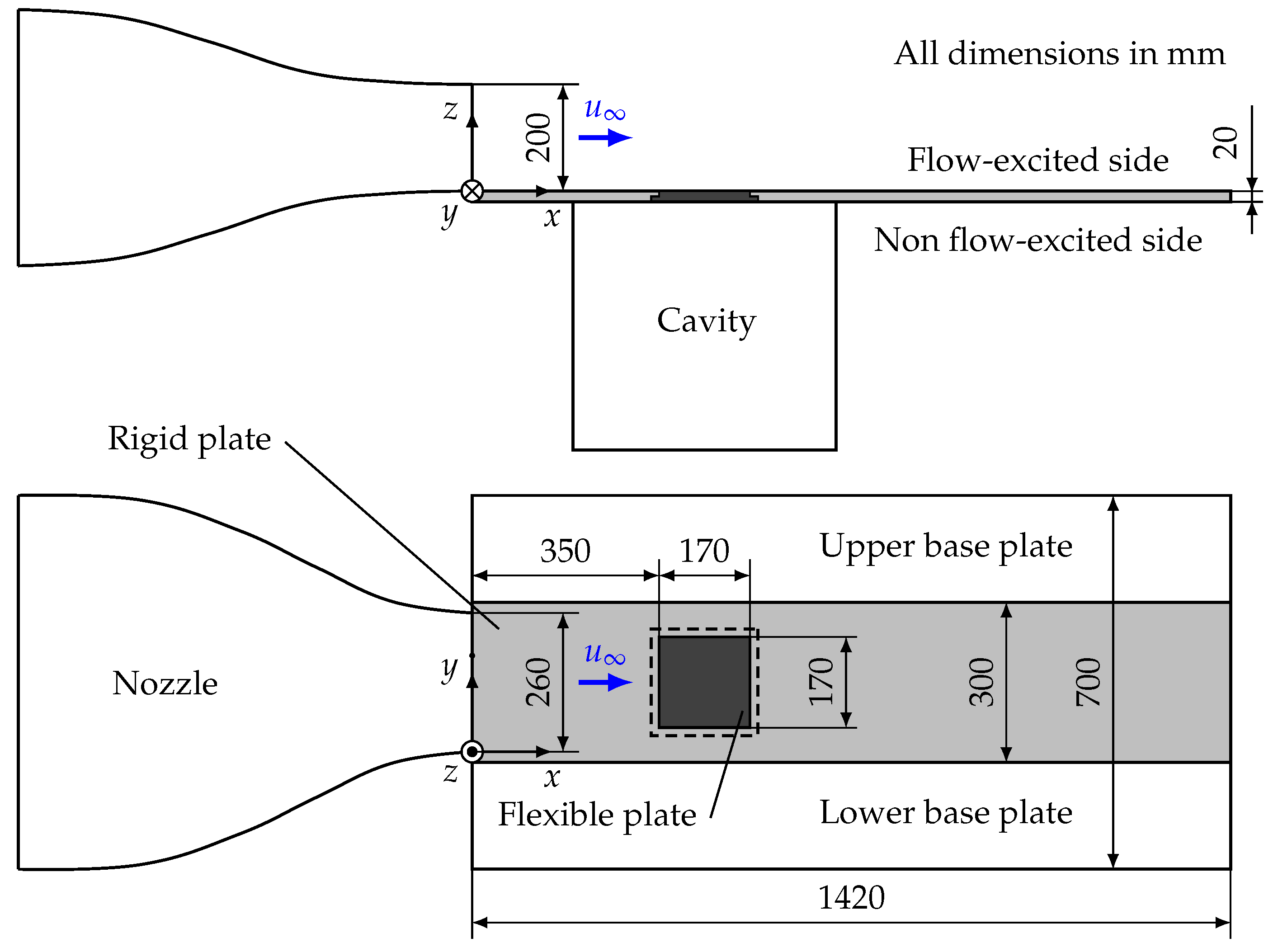
The measurements were performed in the aeroacoustic wind tunnel of the Chair of Sensor Technology at the Friedrich-Alexander University Erlangen-Nürnberg. The measuring section is located in an anechoic room with the dimensions $9\mathrm{m}\times 6\mathrm{m}\times 3.6\mathrm{m}$. The general test setup is installed at a massive base frame built from aluminium profiles to ensure the structural stiffness. To determine the pressure coefficient at the plate surface, 64 holes with the diameter of $0.3\mathrm{m}\mathrm{m}$ are drilled on the flow-exposed surface of the rigid plate, whereas on the other side a threated hole is drilled and tapped to connect pressure hoses to 4 Pressure Systems 16TC/DTC pressure scanners from the company Pressure Systems (Melbourne, Australia). The pressure holes are arranged in a straight streamwise line with a constant spacing from one another. The second measurement setup is shown in Figure 2. The replaced continuous rigid plate is equipped with a square opening in which a manufactured aluminium frame is inserted. The different flexible plates with the thickness $t=1,3$ and $5\mathrm{m}\mathrm{m}$ are each bonded to the frame by an adhesive to avoid possible tensions in contrast to bolting. After installation of the frame, the plane surface of the flexible plate is arranged at the same height as the solid plate. The position of the flexible plate in relation to the nozzle outlet is set so that the entire surface of the plate structure is located in the core area of the free-stream at any time. This substructure ensures that the only way that sound is transferred into the cavity is through the flexible plate.

3.1.2. Sound Field

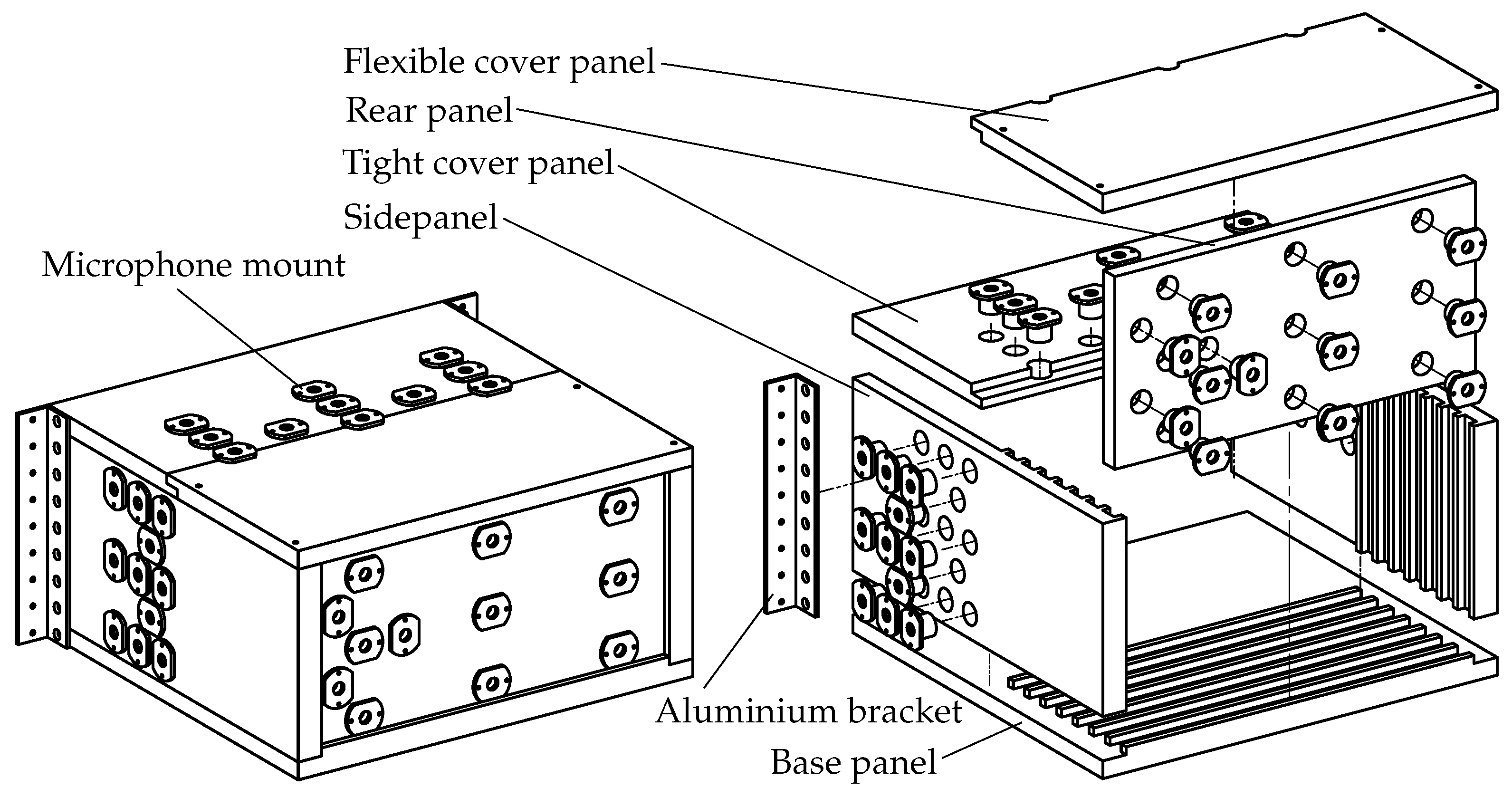
To investigate the sound radiation and transmission of the flexible plate more precisely, a cuboid-shaped room is installed at the back surface of the rigid plate. The outer walls of this cavity are built from $21\mathrm{m}\mathrm{m}$ thick multiplex panels and equipped with microphones to analyze the radiated sound field. The complete mounting and the exploded view are depicted in Figure 3. The cavity volume can be varied by putting the rear panel from above in appropriate recesses at the insides of the sidepanels. The internal dimensions of the cavity are $450\mathrm{m}\mathrm{m}$ × $217\mathrm{m}\mathrm{m}$ × ($255\mathrm{m}\mathrm{m}\mathrm{or}435\mathrm{m}\mathrm{m}$). Consequently, there are two different values for the side length of the cavity, orthogonal to the plate structure. Accordingly, the two obtained different minimum and maximum possible cavity volumes with a room depth of $255\mathrm{m}\mathrm{m}$ and $435\mathrm{m}\mathrm{m}$ are $V_{\min }\approx 0.0249{\mathrm{m}}^3$ and $V_{\max }\approx 0.0425{\mathrm{m}}^3$.

3.2. Measurement Technology and Methods

The wall pressure was measured over a period of $60\mathrm{s}$ with a sampling frequency of $100\mathrm{Hz}$ using the pressure system DTC Initium working with the DTC-technology (Digital Temperature Compensation). To determine the pressure coefficient, 64 positions on the plate in the direction of the flow are simultaneously recorded. The determination of the velocity and of the turbulence intensity is forming the basis for the flow characterization. To approach the true value of the flow velocity as accurately as possible, the velocity regulating differential pressure transducer Model 239 from Setra Systems (Boxborough, Middlesex, MA, USA) is calibrated with the Prandtl Probe TPL-03-200 from KIMO Instruments (Montpon Ménestérol, France) working with very high accuracy. On this basis, the velocity field and the turbulence intensity distribution perpendicular to the flow direction in a certain distance to the nozzle outlet are measured by this Prandtl probe and a hot-wire anemometer with the miniature wire probe 55A53 from Dantec Dynamics (Skovlunde, Denmark).

Using a traversing system, a zero point in the corner of the nozzle outlet is set as a reference for the 108 measurement points. They are arranged on a planar grid, parallel to $yz$-plane with equal spacing. The velocity profiles were measured at distances $x=$ 100, 350 and $520\mathrm{m}\mathrm{m}$ from the nozzle outlet with a sampling rate of $5\mathrm{kHz}$ and a measuring period of $20\mathrm{s}$. The turbulence intensity is determined in the same planes.

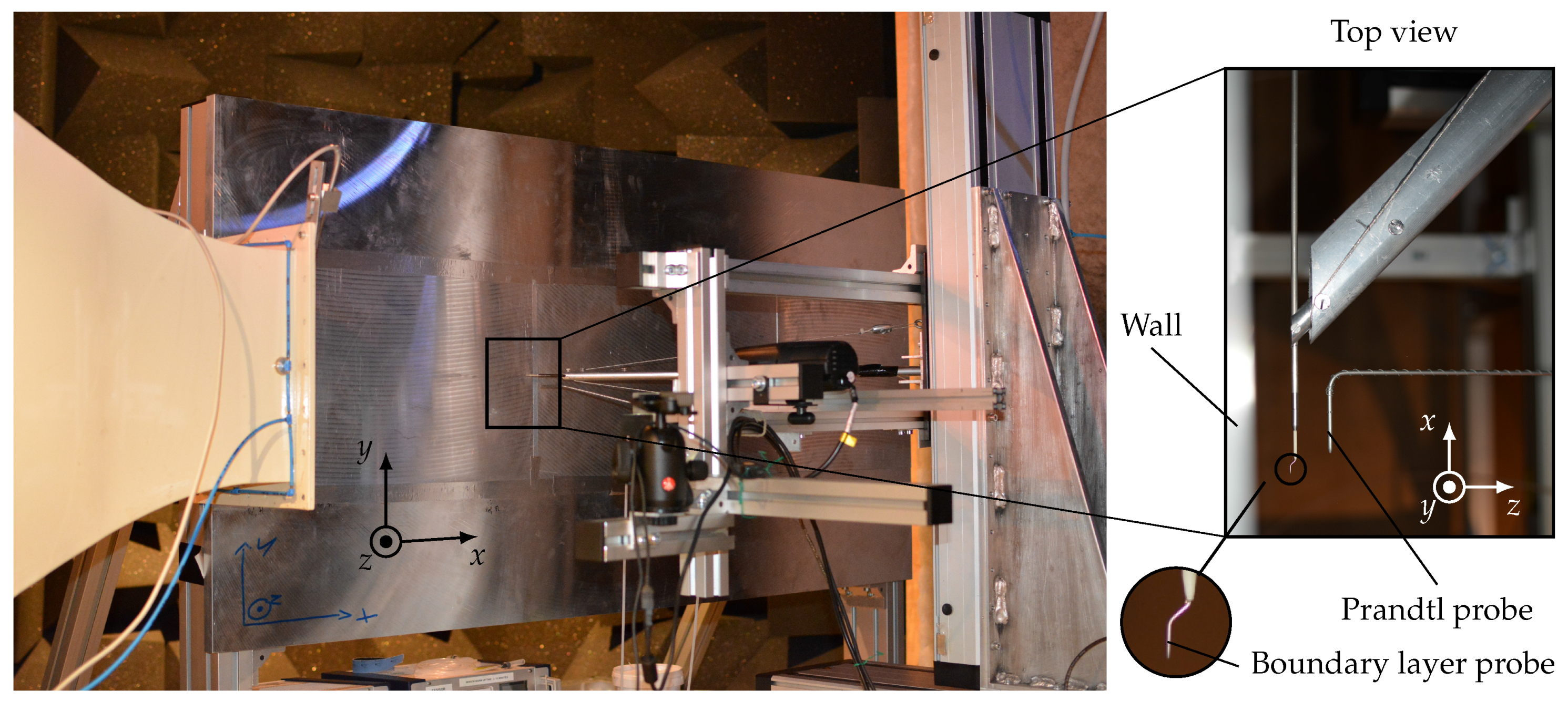
For the examination of the boundary layer, the boundary layer probe 55P15 from Dantec Dynamics is necessary in terms of measurements in direct wall proximity. The corresponding measurement setup with the nozzle, the flow-excited plate and the traversing system is shown in Figure 4. The measurement distances to the nozzle are chosen between the position of the front edge ($x=350\mathrm{m}\mathrm{m}$) and the rear edge ($x=520\mathrm{m}\mathrm{m}$) of the installed flexible plate. More precisely, different not equidistant points in z-direction perpendicular to the plate are measured. While approaching towards the wall, the distance is successively decremented. The traversing system automatically moves the probe to all points till the contact point between probe and plate is reached.

The microphones in the side panel and the top panel are arranged in such a way that they are able to collect the generated noise at anytime independent of the rear panel position. Moreover, one microphone row is placed in the middle of the minimum and the maximum volume in each case. The cavity volume and the microphone measuring positions are varied for the same plate thickness of the flexible plate structure. This results in different measuring configurations with the following variation possibilities:

• Cavity volume:       minimum and maximum
• Microphone arrangement:  left, top and rear
• Flow velocity:        $45\mathrm{m}{\mathrm{s}}^{-1}$
• Plate thickness:       $1\mathrm{m}\mathrm{m}$, $3\mathrm{m}\mathrm{m}$ and $5\mathrm{m}\mathrm{m}$

Additionally, a frame, milled from solid with a thickness of $20\mathrm{m}\mathrm{m}$, is precisely closing the square opening in the rigid aluminium plate and has been prepared for comparative purposes. It can be assumed that there is no noise transmitted through this frame.

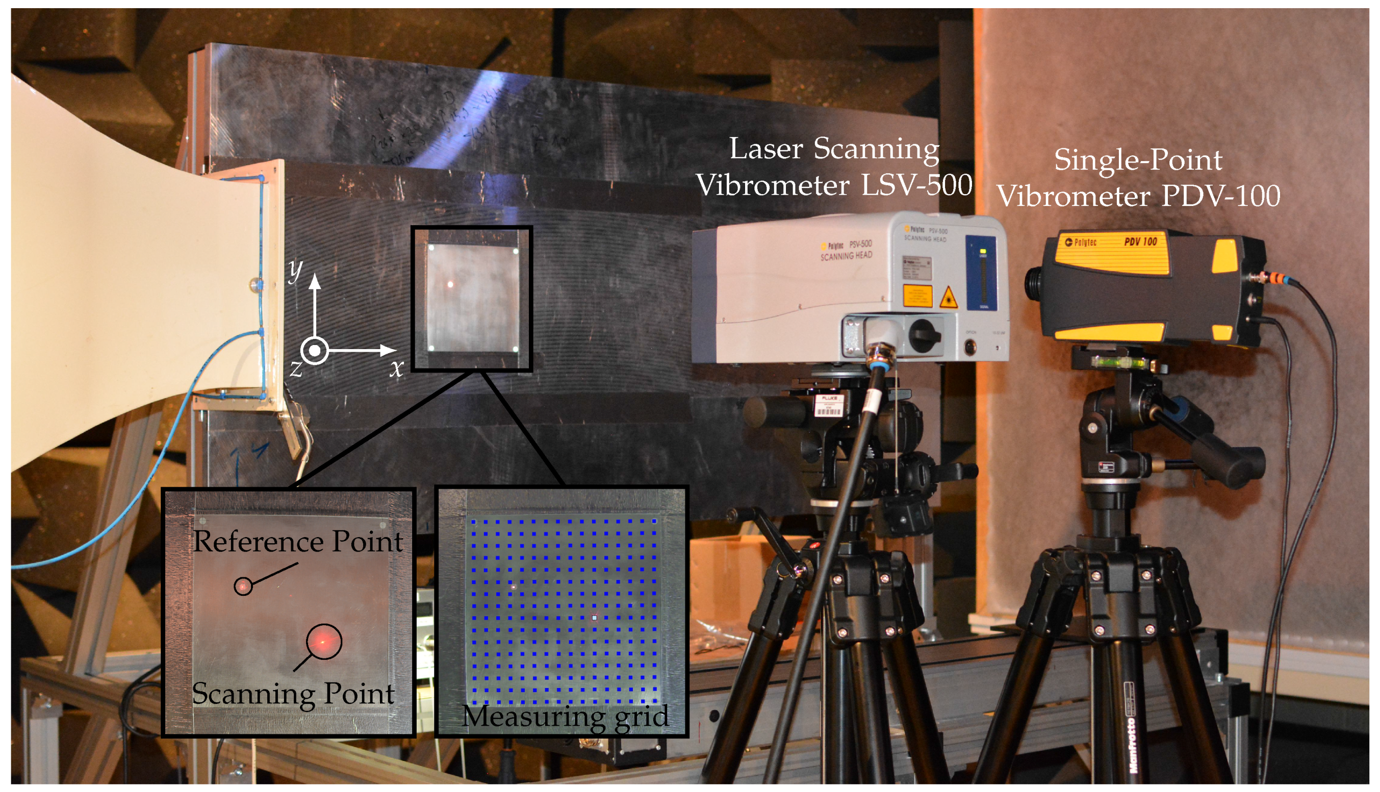
To detect structural vibrations of the flexible plate and to establish a correlation with the sound radiation in the cavity, Laser Scanning Vibrometer measurements are performed. The method is based on the Doppler-effect where two coherent light beams with different path lengths overlap and result in optical interference. The velocity of a certain point on the vibrating plate is determined through the known wavelength of the laser beam and the frequency shift due to the motion of the surface (Figure 5).

A square-shaped grid with 256 measuring points is generated and placed on the surface of the flexible plate using the Laser Scanning Vibrometer PSV-500 from Polytec (Waldbronn, Germany) with an automatic scanning mirrors system. To accurately replicate the structural modes of the plate, the phase relation of each measuring point to one fixed point is required. Therefore, the Single-Point Vibrometer PDV-100 from Polytec is connected to the first reference input channel of the data acquisition card of the PSV-500 Scanning System. Flush-mounted microphones are also used as reference signals.

4. Experimental Results

The experimental results of all measurements are presented and interpreted in this section.

4.1. Flow Characterization

Initially, the flow directly influencing and exciting the flexible aluminium plate was examined in detail in the following two subsections. In particular, different flow parameters and the boundary layer on the flow-excited surface of the flexible plate have been investigated.

4.1.1. Flow Parameters

In general, the wind pressure merely acts towards the plate surface and thus, the pressure coefficient achieves positive values. The results show that first there is a sharp decline till the pressure coefficient is reaching a certain level. This suggests that the flow is not fully turbulent developed yet, but the transition area between laminar and turbulent flow is still present. A rough calculation of the critical Reynolds number confirms this assumption. In conclusion, there is no boundary layer with zero pressure gradient because the pressure coefficient is not close enough to zero. However, the values are only slightly increasing above 0.01 so that the deviation is relatively small. The relevant range between the front edge and the trailing edge of the flexible plate shows the least fluctuating pressure coefficient with values between 0.005 and 0.01. Consequently, the boundary layer along a flat plate is characterized by the fact that the velocity profiles measured at different distances to the leading edge of the rigid plate are similar.

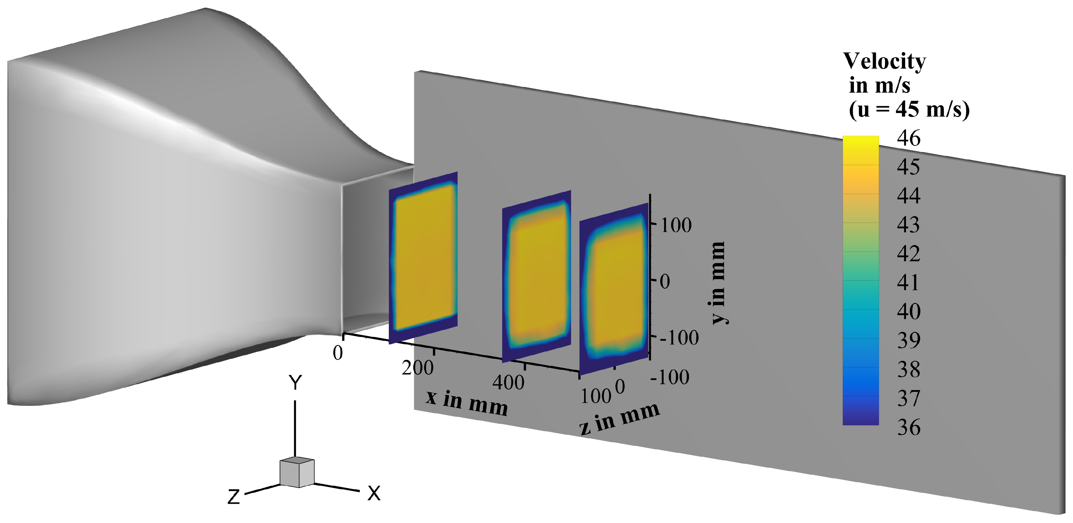
The spatial distribution and the accuracy of the flow velocity is very important in the aeroacoustic wind tunnel because the validity of the measurements is strongly dependent on whether a uniform velocity field with nearly constant velocity in the core region is formed in the test section. The resulting velocity profiles are depicted in Figure 6 by means of contour plots linked to a simplified CAD model of the nozzle and the rigid plate. It is shown that the core area of the flow with a nearly constant velocity is shrinking, whereas the mixing zone in the transition area to the resting medium is broadening. The flow-excited flexible plate, which is exactly located between the two velocity profiles at x = 350 and $520\mathrm{m}\mathrm{m}$, is clearly lying in the core flow.

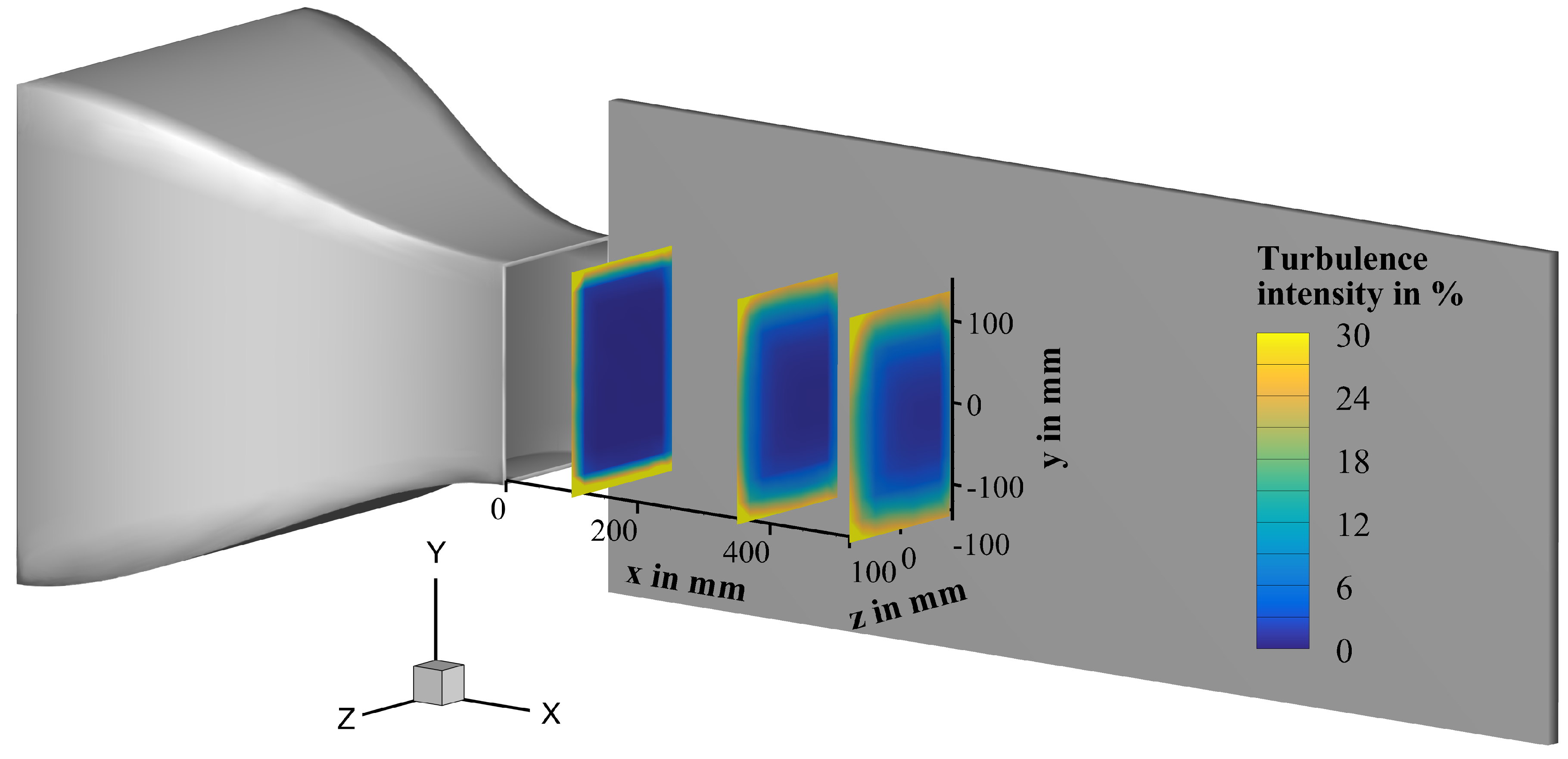
The turbulence intensity for isotropic turbulence with equal average velocity fluctuations in all three dimensions ${u_x^{\prime }}^2={u_y^{\prime }}^2={u_z^{\prime }}^2$ [9,15] is

$$T_u=\frac{\sqrt{\overline{{u_x^{\prime }}^2}}}{u_{\infty }}\times 100\mathrm{in}\%$$

(16)

The distribution of the increasing turbulence intensity from 0 towards the edges is similiar to the decreasing velocity from $45\mathrm{m}{\mathrm{s}}^{-1}$ (Figure 6). Moreover, the turbulence intensity is identically depicted as the velocity profiles (Figure 7) at the same position. The turbulence intensity values at the edges increase with distance to the nozzle. Accordingly, a contour with relatively small width and increased turbulence intensity, which is recreating the form of the nozzle outlet, is growing in width towards the middle of the profile. The first contour plot shows a high turbulence intensity at the edges. Considering the contour plots at the position x = $350\mathrm{m}\mathrm{m}$ and $520\mathrm{m}\mathrm{m}$, the turbulence intensity at the edges decreases with increasing distance to the nozzle. As already mentioned in connection with the flow velocity, a good comparability and transferability of the measurement results can be provided because the area of the flexible plate structure is exposed to low turbulence.

4.1.2. Boundary Layer

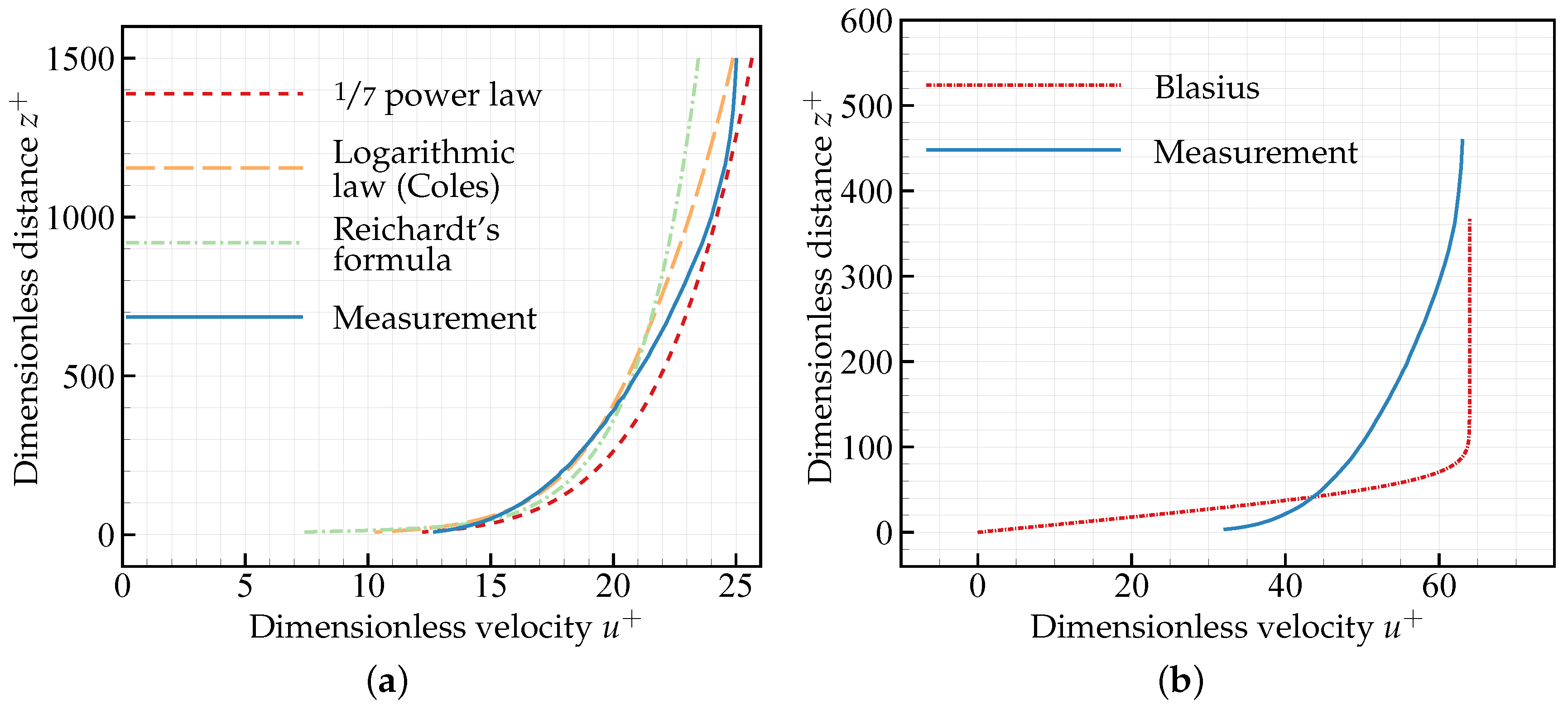
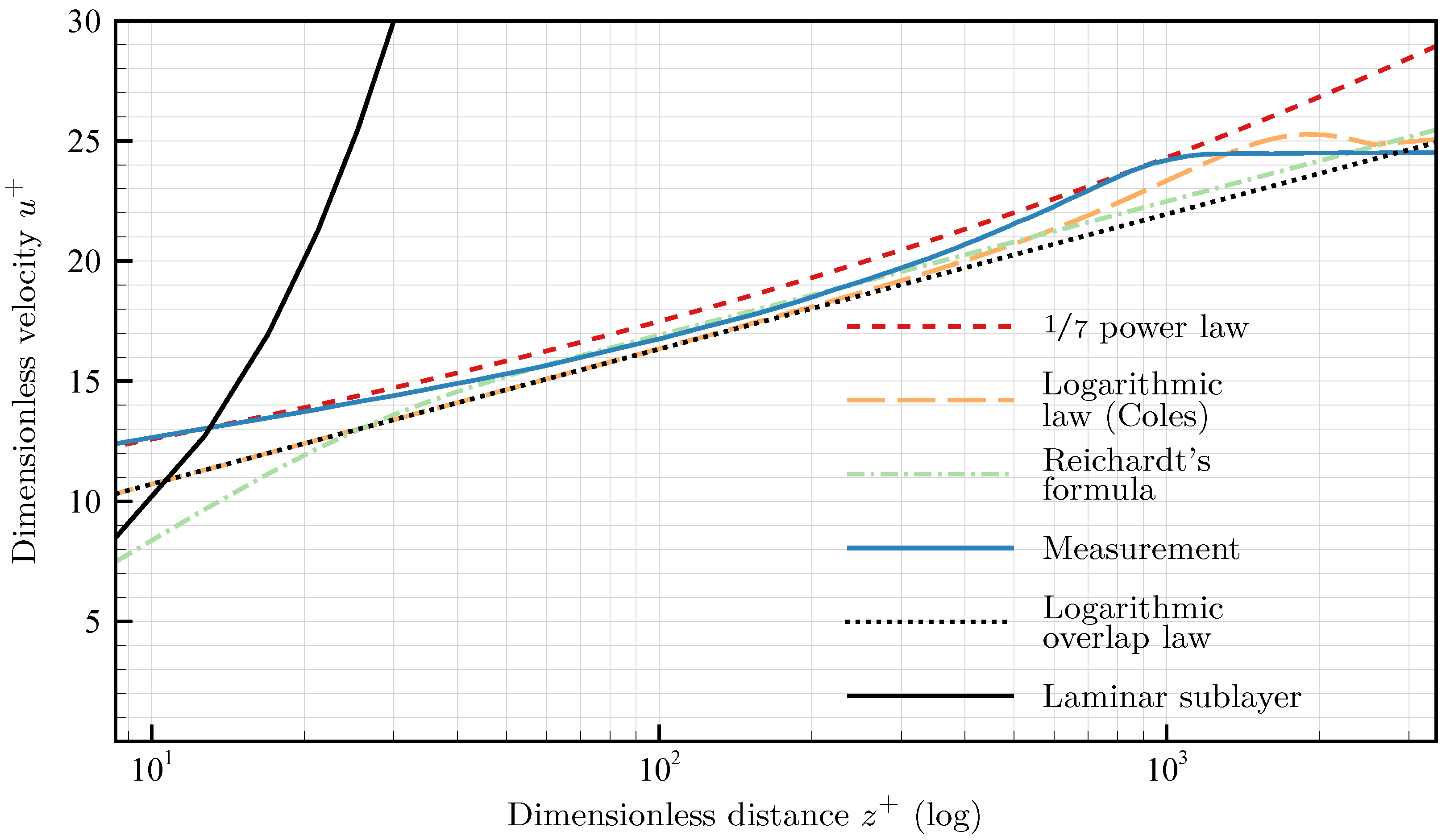
The dimensionless velocity profiles of the measurement, of the three indirect turbulence models and of the approach after Blasius (refer to Section 2) for a distance to the nozzle outlet of $x=350\mathrm{m}\mathrm{m}$ are shown in Figure 8. The turbulence models correlate in exponential curve characteristics compared with the measurement in contrast to the approach after Blasius which shows a linearly increasing course at the beginning changing to an exponential growth till the maximum value of $u^{+}$. This result suggests that the boundary layer is turbulent.

To evaluate the quality of the indirect turbulent models more clearly, another depiction of the dimensionless velocity profiles of the turbulent presumed boundary layer is presented in Figure 9. Besides this, the graphs of the logarithmic overlap law and of the laminar sublayer are added. The $1/7$ power law reproduces the curve shape of the measurement most closely at the beginning, whereas the logarithmic law after Coles overlaps the measurement between a dimensionless distance from $z^{+}=$ 90 to 200. Towards the end, a plateau with constant dimensionless velocity is to be noticed which means that this section is already outside of the boundary layer. The curve progressions of the logarithmic law and the logarithmic overlap law are the same till reaching the outer part of the boundary layer. There, the law of the wake as the third summand added to the logarithmic overlap law takes effect and describes the outer part in the corrected equation of Coles (Equation (8)). The laminar sublayer completely deviates from the other curves.

The shape factor $H_{12}$ as the ratio of the displacement thickness ${\delta }_1$ to the momentum loss thickness ${\delta }_2$ is used to characterize the boundary layer developing on a flat plate. The integral calculation of the displacement thickness ${\delta }_1$ and the momentum loss thickness ${\delta }_2$ is done by a spline interpolation with a following exact numerical integration using global adaptive quadrature and preset fault tolerance [16]. The values of $H_{12}$ converge towards 1.3 despite varying values for ${\delta }_1$ and ${\delta }_2$ for different x-positions. For laminar flows on a flat plate, $H_{12}$ is typically about 2.59. At the transition point it falls to a considerably smaller number range between 1.4 and 1.0 [9,17]. Clauser [18] concluded that $H_{12}$ is dependent on the Reynolds number ${Re}_x$ based on the running length x and on the skin friction coefficient $C_f$ for equilibrium boundary layers. In this case of constant pressure profiles, for a range of ${10}^6<{Re}_x<{10}^7$, the values of $H_{12}$ are expected to be between 1.27 and 1.35 with $C_f$ between 0.025 and 0.036. According to Head, Coles and Smith and Walker [19] $H_{12}$ assumes higher values between 1.3 and 1.42 in the same range of ${Re}_x$. Nikuradse [20] concluded after measuring the boundary layer for a pipe flow that $H_{12}$ = 1.3 is constant in the measurement range of $1.7\times {10}^6\le {Re}_x\le 1.8\times {10}^7$. All boundary layer parameters are shown in

Table 1. Boundary layer parameters for the analytical approaches.

$\mathit{x}-\mathbf{pos}.$	${\mathit{x}}_{\mathbf{new}}$	${\mathit{u}}_{\mathbf{\infty }}$	${\mathit{u}}_{{\mathit{\tau }}_1}$	${\mathit{\delta }}_{100}$	${\mathit{\delta }}_1$	${\mathit{\delta }}_2$	${\mathit{H}}_{12}$	${\mathit{R}\mathit{e}}_{\mathit{x}}=$	${\mathit{R}\mathit{e}}_{{\mathit{\tau }}_1}=$	${\mathit{R}\mathit{e}}_{{\mathit{\delta }}_2}=$
$\mathbf{mm}$	$\mathbf{mm}$	$\mathbf{m}{\mathbf{s}}^{-\mathbf{1}}$	$\mathbf{m}{\mathbf{s}}^{-\mathbf{1}}$	$\mathbf{mm}$	-	-	-	${\mathit{u}}_{\infty }{\mathit{x}}_{\mathbf{new}}/\mathit{\nu }$	${\mathit{u}}_{\mathit{\tau }}{\mathit{\delta }}_{\mathbf{100}}/\mathit{\nu }$	${\mathit{u}}_{\infty }{\mathit{\delta }}_{\mathbf{2}}/\mathit{\nu }$
350.0	702.2	45.00	1.80	14.44	1.80	1.38	1.30	1.91 $\times {10}^6$	1571	3.76 $\times {10}^6$
392.5	721.7	45.01	1.79	14.77	1.89	1.45	1.31	1.96 $\times {10}^6$	1598	3.93 $\times {10}^6$
435.0	807.7	45.01	1.78	16.18	2.07	1.58	1.31	2.18 $\times {10}^6$	1722	4.26 $\times {10}^6$
477.5	859.4	45.01	1.77	17.01	2.22	1.70	1.31	2.31 $\times {10}^6$	1796	4.58 $\times {10}^6$
520.0	977.8	45.01	1.74	18.87	2.41	1.83	1.31	2.63 $\times {10}^6$	1963	4.92 $\times {10}^6$

. The resulted values of $H_{12}$ clearly prove that there is a turbulent flow in the entire area of the flexible flow-excited plate. Moreover, the calculated x-distance $x_{\mathrm{new}}$ from Equation (15) is nearly twice as high as the real x-position. The boundary layer thickness ${\delta }_{100}$ increases with the distance to the nozzle.

The measurement data is fitted using the approach from Golliard [12] to reproduce the curve progression of the dimensionless velocity most accurately. The generated curve points based on the spline interpolation are entered as input data for the curve fitting using the least squares method. The logarithmic law from Equation (8) is the objective function, in which $u_{\infty }$ is replaced by the velocity at the boundary layer border from the hot-wire measurements $u_0$. The z-distance is the passed dependent variable and the four fit variables are $u_0$, $u_{{\tau }_{\mathrm{Go}}}$, ${\delta }_{100}$ and $z_0$ with the Levenberg-Marquardt algorithm as numeric optimization method [21,22]. Another curve fitting with constant $u_0$ and ${\delta }_{100}$ and only $u_{{\tau }_{{\mathrm{Go}}_2}}$ and $z_0$ as fit parameters is performed to verify the quality of the results.

Comparing the wall shear stress resulting from the analytical calculation ($u_{{\tau }_1}$, $u_{{\tau }_2}$) with those from the numerical approximation ($u_{{\tau }_{\mathrm{Go}}}$, $u_{{\tau }_{{\mathrm{Go}}_2}}$), one can recognize different values as shown in

Table 2. Comparison of the boundary layer parameters to analytical approaches and to the curve fitting beyond the approach of Golliard.

$\mathit{x}-\mathbf{pos}.$	${\mathit{u}}_0$	${\mathit{u}}_{{\mathit{\tau }}_1}$	${\mathit{u}}_{{\mathit{\tau }}_2}$	${\mathit{u}}_{{\mathit{\tau }}_{\mathbf{Go}}}$	${\mathit{u}}_{{\mathit{\tau }}_{{\mathbf{Go}}_2}}$	${\displaystyle \frac{{\mathit{u}}_{{\mathit{\tau }}_1}}{{\mathit{u}}_{\infty }}}$	${\displaystyle \frac{{\mathit{u}}_{{\mathit{\tau }}_2}}{{\mathit{u}}_{\infty }}}$	${\displaystyle \frac{{\mathit{u}}_{{\mathit{\tau }}_{\mathbf{Go}}}}{{\mathit{u}}_0}}$	${\displaystyle \frac{{\mathit{u}}_{{\mathit{\tau }}_{{\mathbf{Go}}_2}}}{{\mathit{u}}_0}}$
$\mathbf{mm}$	$\mathbf{m}{\mathbf{s}}^{-\mathbf{1}}$	$\mathbf{m}{\mathbf{s}}^{-\mathbf{1}}$	$\mathbf{m}{\mathbf{s}}^{-\mathbf{1}}$	$\mathbf{m}{\mathbf{s}}^{-\mathbf{1}}$	$\mathbf{m}{\mathbf{s}}^{-\mathbf{1}}$	-	-	-	-
350.0	44.11	1.799	1.823	1.758	1.792	0.040	0.041	0.040	0.041
392.5	43.87	1.795	1.819	1.733	1.763	0.040	0.040	0.039	0.040
435.0	44.44	1.776	1.799	1.730	1.767	0.039	0.040	0.039	0.040
477.5	43.99	1.765	1.789	1.704	1.739	0.039	0.040	0.039	0.040
520.0	43.78	1.743	1.766	1.664	1.707	0.039	0.039	0.038	0.039

. However, relating to their respective velocities ($u_{\infty }$, $u_0$), nearly equal values are obtained. It can thus be concluded that the Equations (2) and (6) for the wall shear stresses ${\tau }_{w_1}$ and ${\tau }_{w_2}$ provide a very good approximation. The adapted running length $x_{\mathrm{new}}$ (Equation (15)) and the boundary layer thickness ${\delta }_{100}$ (Equation (3)) are used for the calculation. Without measurement data it is impossible to calculate or predict the boundary layer parameters in case of an artificially induced turbulent boundary layer, whereas the adjusted analytical approaches solely suffice to characterize the boundary layer with the existance of measurement data.

4.2. Flow-Induced Sound Radiation into the Cavity

To determine the influence of the single measuring configurations and to compare and assess those effects, there are only one or two varying parameters. All figures are related to microphone position number 5 which is each located in the middle of the rear, side and top panel of the cavity (Figure 10). Unless otherwise specified, the maximum volume and the microphone position on the rear panel is chosen in the following. The lower cut-off frequency of the cavity as an acoustic chamber with maximum volume is $2866\mathrm{Hz}$. Above this frequency, a strong superpositioning of natural frequencies occur which is apparent in the following sound pressure level depictions.

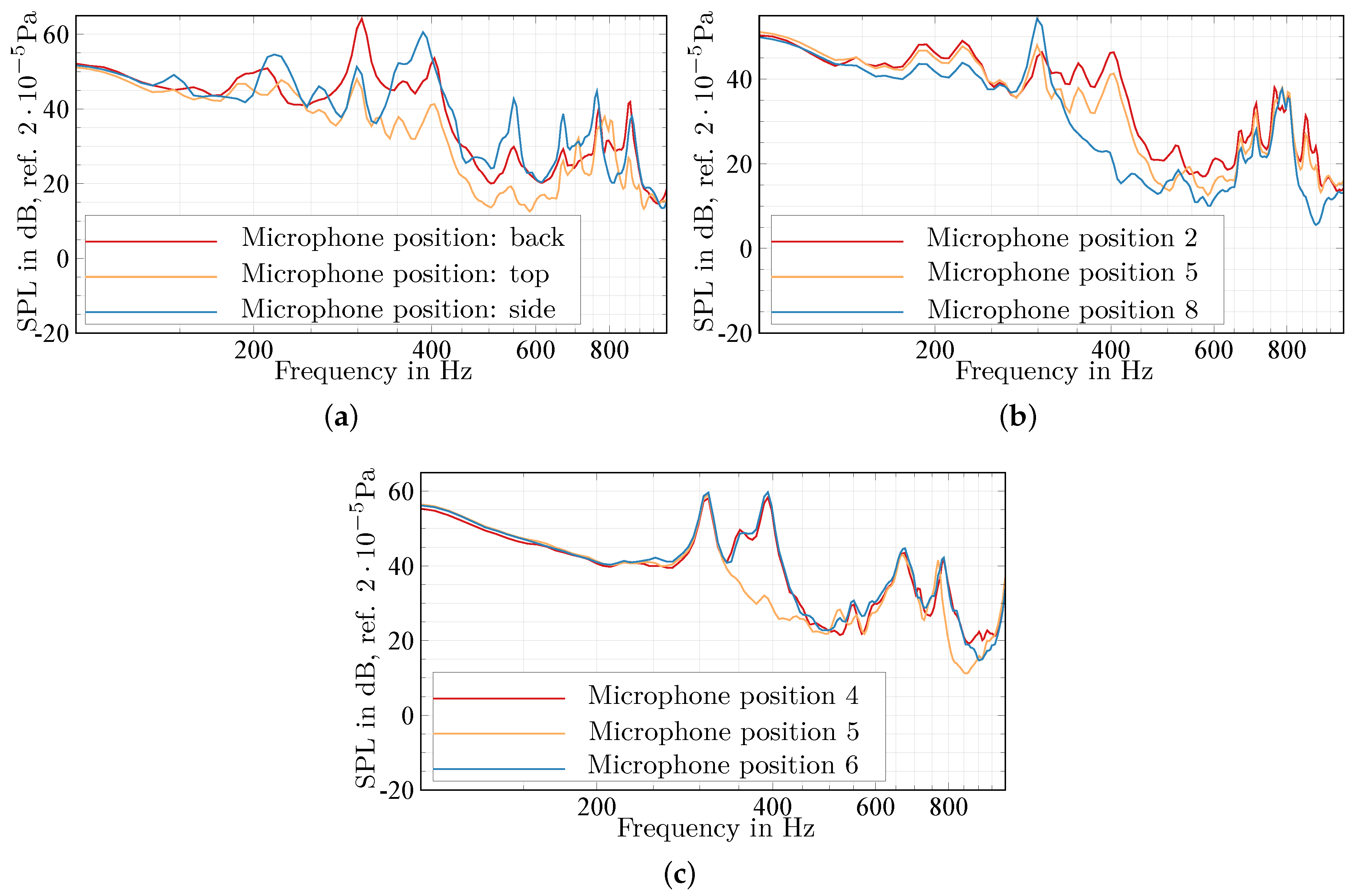
Figure 11 shows the effects of different microphone positions on the sound pressure levels. The measuring planes (Figure 11a), the distance from the flexible plate (Figure 11b) and finally the microphone position in the rear panel (Figure 11c) are varied. The frequency range is from 100 to $1000\mathrm{Hz}$ because that is the interesting area where significant modifications arise. The sound pressure level spectrum is plotted against the frequency for the three microphone positions on the different cavity walls.

Common peaks appear in Figure 11a at $310\mathrm{Hz}$, in the range of $400\mathrm{Hz}$, $550\mathrm{Hz}$ and at higher frequencies, too. Below $300\mathrm{Hz}$, the curve characteristics differ considerably because the frequency is below the frequency of the first room mode of the cavity and thus not influenced by the room.

The second figure (Figure 11b) depicts the different distances from the flexible plate with position 2 as the nearest position to the plate. Between 300 and $500\mathrm{Hz}$, the sound pressure level measured at position 8, located at half of the cavity length, is significantly lower than those of the other positions. This is because special acoustic waves, whose wavelength correspond to the half room length, form nodes and thus sound pressure minima. A greater distance to the flexible plate leads to a lower sound pressure level at low frequencies with the exception of a few peaks.

Finally, different x-positions, describing the distances from the nozzle outlet in streamwise direction, are selected and located on the rear panel. The distance increases with a decreasing microphone number while number 5 exactly represents the perpendicularly displaced center of the flexible plate. There is a lower sound pressure level between the microphone positions 4 and 6 compared with 5 between 330 and $450\mathrm{Hz}$ and between 770 and $900\mathrm{Hz}$. The responsible axial modes run in negative z-direction from the flexible plate and produce sound pressure minima at position 5. The curve shapes up to a frequency of $330\mathrm{Hz}$ in the low-frequency range are similar to each other.

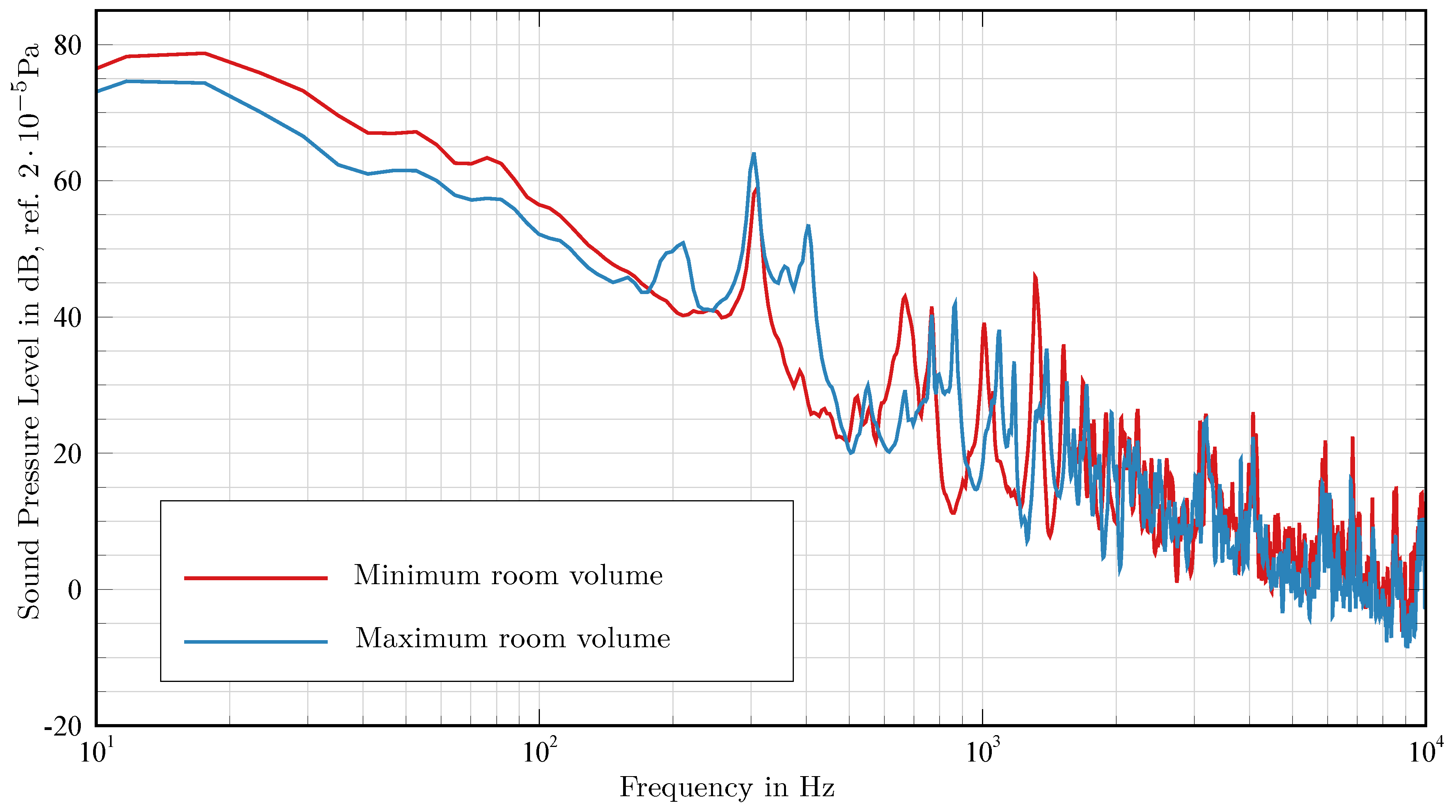
Changing the rear panel position and thus the cavity volume implicates different developing sound pressure levels (Figure 12). The maximum at $210\mathrm{Hz}$ only occurs with maximum volume although cavity modes do not propagate below the first axial mode at approximately $400\mathrm{Hz}$. This sound superelevation is dependent on the room size and position. The small peak at a frequency of $387\mathrm{Hz}$ can be explained by the second axial room mode for the minimum cavity volume.

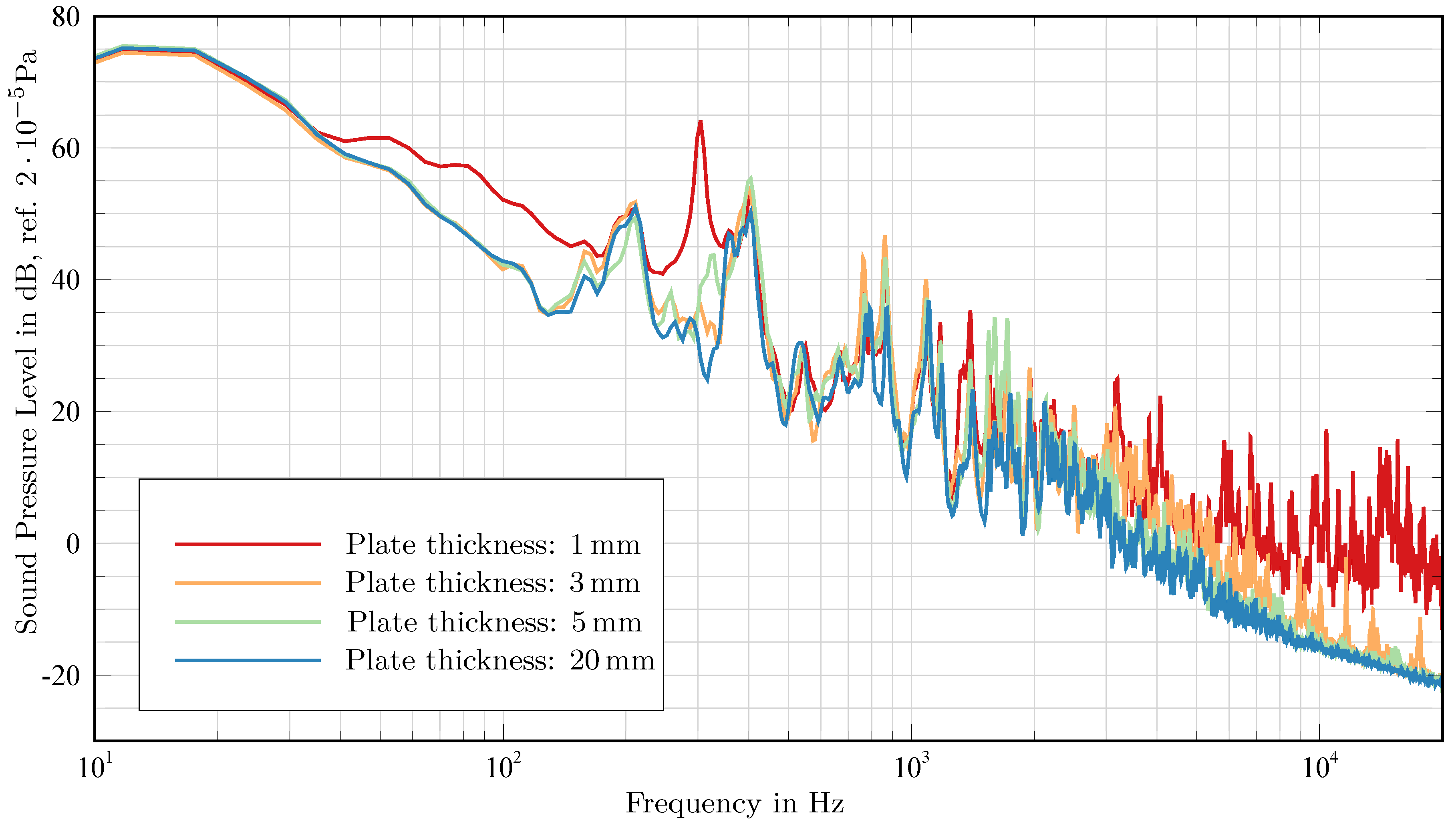
The next step was to study the influence of plate thickness variation which is depicted in Figure 13. There is a considerable difference in the development of the sound pressure level at low frequencies for a plate thickness of $1\mathrm{m}\mathrm{m}$ and the remaining thicknesses. The shape modes of the thinnest plate are excited and radiate sound into the cavity. Furthermore, the sound transmission through this plate is the highest among the other thicker plates. The first two peaks at 160 and $210\mathrm{Hz}$ appear regardless of the thickness and only for maximum volume. Subsequently, their development is not associated with the natural frequency of the thinnest plate. An immense sound pressure level variation is shown at $310\mathrm{Hz}$. Whereas there are only small impacts on the medium thick plates at this point, a huge positive peak is shown for the $1\mathrm{m}\mathrm{m}$ thick plate and on the contrary a negative peak for the $20\mathrm{m}\mathrm{m}$ thick solid plate. The short-circuit area and the piston-diaphragm area are located below the first natural frequency of the thinnest plate at $217.4\mathrm{Hz}$. Thus, the increase can be explained by the sound transmission through the plate structure. At higher frequencies above $3000\mathrm{Hz}$, the sound pressure level is increasing with a reduction of the plate thickness due to a different degree of oscillation excitation and varying sound transmission strength. Additionally, the illustrated frequency spectrum is extended to $20\mathrm{k}\mathrm{Hz}$ to show the sound pressure increase from approximately 12,800 $\mathrm{Hz}$ for the $1\mathrm{m}\mathrm{m}$ thick plate. This is caused by the coincidence frequency above which a full sound radiation occurs. This effect is superimposed by other sound sources for the remaining plate thicknesses. Finally, the common peak at $550\mathrm{Hz}$ is due to the first tangential room mode.

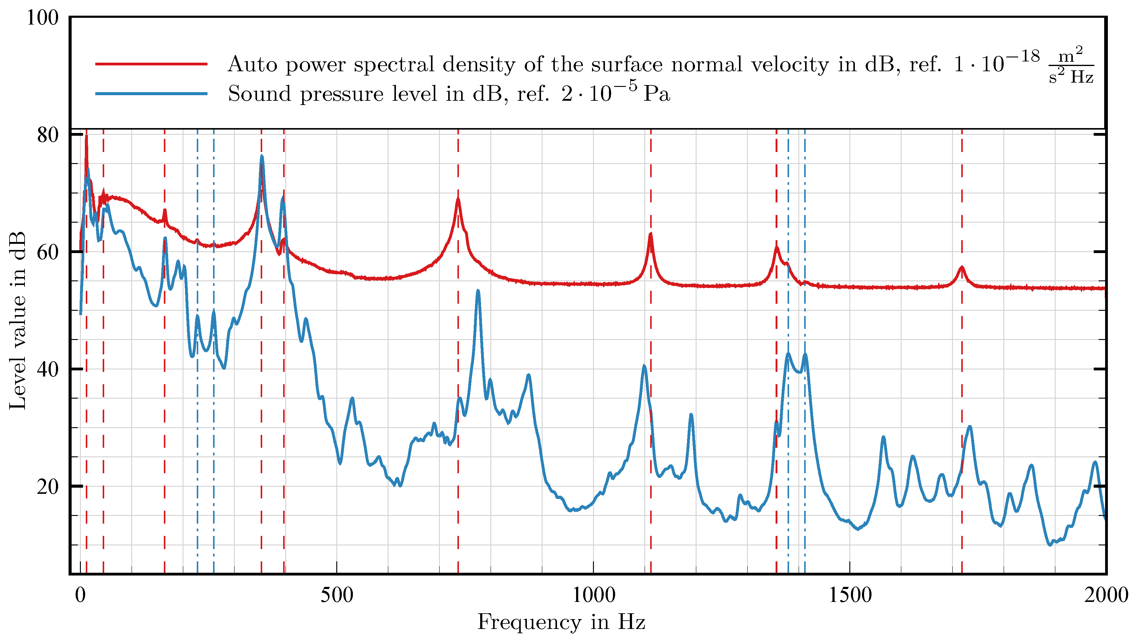
To evaluate the mutual influence of the vibrating plate and the cavity, the auto power spectral density (APSD) of the surface normal velocity of the single-point vibrometer and the sound pressure level (SPL) of the microphone which is located in the middle of the rear panel are depicted together in Figure 14. The APSD is calculated as follows:

$${\displaystyle \mathrm{APSD}=10{log}_{10}\frac{{\displaystyle \frac{1}{{\displaystyle (\mathrm{signal}\mathrm{length})·(\mathrm{sampling}\mathrm{frequency})}}·{|\mathrm{fft}(\mathrm{x})|}^2}}{{10}^{-18}}}$$

(17)

with the signal length of 3200 and the sampling frequency of $2000\mathrm{Hz}$. They are both converted to the unit but have two different reference values concerning the level calculation. There are 9 vertical dashed red lines representing the highest peaks of the APSD and 4 vertical dash dotted blue lines which show peaks of the SPL and small influences in the APSD at identical frequencies.

In the low frequency range till approximately $400\mathrm{Hz}$, numerous maximum values of both curves appear at the same frequency in contrast to higher frequencies. Plate vibrations which occur below the first natural frequency of the plate at $353.125\mathrm{Hz}$ develop due to coupling with the entire frame structure of aluminium and pressurisation which is caused by low-frequency vortices.

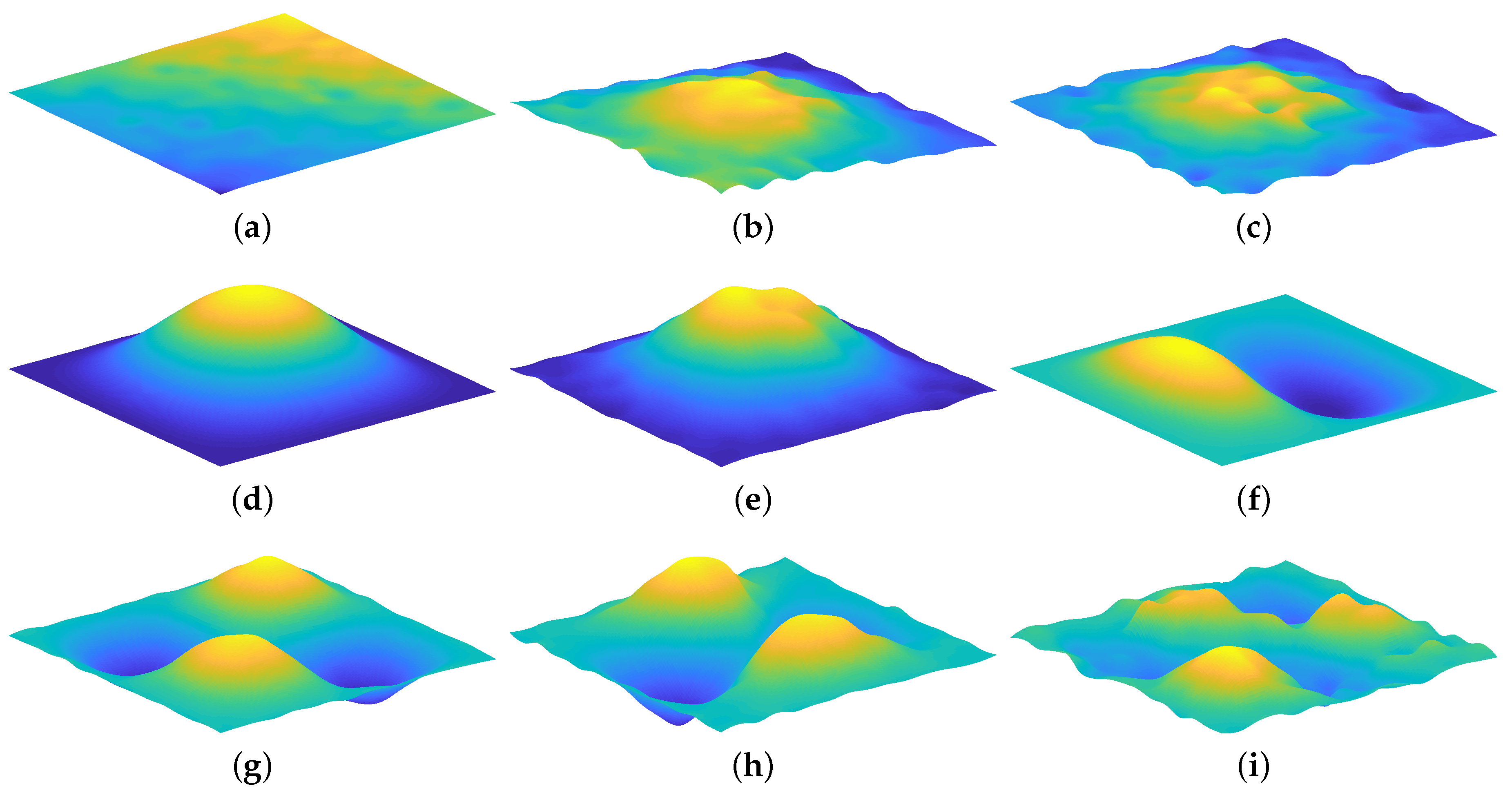
The first peak at $f=11.875\mathrm{Hz}$ which is depicted in Figure 15a results from a vibration of the entire system which can be derived from the chronological sequence of the plate vibration. Every measurement point of the plate is oscillating with the same amplitude and phase. In the second Figure (Figure 15b), a superimposition between the vibration of the plate and a the formation of a kind of structural oscillation occurs although the first shape mode firstly appears at a higher frequency. The front area of the flow-excited plate, which is closer to the nozzle outlet, is considerably stronger oscillating upwards and downwards towards the surface normal than the rear region. The movement of the plate’s rear edge is lagging behind the front edge like the phase-shifted points of a standing wave. The plate tilts whenever the front or the rear edge reaches the maximum oscillation amplitude. It is exposed to a compressive and tensile load caused by vortex structures with a long wavelength. The maximum value of the APSD is not clearly noticeable and has a higher peak width. The third peak of the APSD and the SPL results in a vibration form $f=164.375\mathrm{Hz}$ in Figure 15c. The bending of the plate moves in streamwise direction. One reason for the occuring mode shape across a wide frequency range which is similar to the first shape mode at $f=353.125\mathrm{Hz}$ (Figure 15d) is the increasing convection velocity with increasing frequency in the low frequency region [23]. Thus, the wavelength of the large eddies is slightly changing, whereby the effect on the plate remains similar. The vibration of the flexible plate leads to a sound radiation into the cavity which occurs at the first shape mode. Conversely, the first axial room mode at $f=397\mathrm{Hz}$ in Figure 15e appears in form of a peak in the SPL of the microphones and the APSD of the surface normal velocity. The plate is oscillating, induces the room mode, which in turn excites the plate to vibrate at the same frequency. The same phenomenon arises on a smaller scale at the frequencies which are highlighted by the 4 vertical dash dotted blue lines. The second shape mode at $f=736.25\mathrm{Hz}$ in Figure 15f has similarly to the following plate modes (Figure 15g–i) only a minor impact on the sound pressure level in the cavity.

In summary, the first shape mode has the greatest influence on the sound pressure level in the cavity. Moreover, the larger peaks of the APSD of the surface normal velocity match with those of the SPL in the low frequency region. The vibrations of the plate or the entire system with a higher amplitude are transferred into the cavity and influence the inner sound pressure level.

5. Conclusions

In this paper, measurements to characterize the flow and to determine the vibration and sound radiation of flexible plate structures into cavities are recorded. Moreover, the corresponding results are discussed. In summary, the flow is clearly defined by the analytical and numerical approaches. The velocity profiles and the turbulence intensity distribution reproduce the rectangular geometry of the nozzle outlet, are uniformly developed, but show wider edges with deviation from the optimum range. However, the flow-excited flexible plate structure is completely located in the core area of the open jet. The type of the flow along the plate is demonstrably a turbulent boundary layer which is proved by the shape factor $H_{12}$. To describe the boundary layer through the measurement data, the adapted analytical approaches suffice. The analysis of the flow-induced sound radiation into the cavity yields to different results depending on the measuring configuration. The highest sound pressure levels in the cavity are detected at the thinnest plate $t=1\mathrm{m}\mathrm{m}$. This can be seen both in the low frequency and the high frequency region and especially at $310\mathrm{Hz}$. With the laser scanning vibrometer measurements, correlations between the vibration of a plate, the sound radiation and the retroactive effect of the cavity could be captured.

The aim of all the efforts is to understand the entire effect chain from the plate excitation to the sound detection for which fundamental knowledge is required. These includes basic experiments which were carried out in the present study. The measurements should serve as a benchmark for future tests. Adding another flexible plate behind the first one and testing different materials could provide more knowledge about multilayer constructions like already in use in nearly all vehicles.

References

- Schulte-Fortkamp, B.; Jakob, A.; Volz, R. Lärm Im Alltag-Informationsbroschüre Zum Tag Gegen Lärm; Deutsche Gesellschaft für Akustik e.V. (DEGA): Berlin, Germany, 2011. [Google Scholar]
- Purohit, A.; Darpe, A.K.; Singh, S. Experimental Investigations on Flow Induced Vibration of an Externally Excited Flexible Plate. J. Sound Vib. 2016, 371, 237–251. [Google Scholar] [CrossRef]
- Sadri, M.; Younesian, D. Vibro-Acoustic Analysis of a Coach Platform under Random Excitation. Thin Walled Struct. 2015, 95, 287–296. [Google Scholar] [CrossRef]
- Shi, S.; Su, Z.; Jin, G.; Liu, Z. Vibro-Acoustic Modeling and Analysis of a Coupled Acoustic System Comprising a Partially Opened Cavity Coupled with a Flexible Plate. Mech. Syst. Signal Process. 2018, 98, 324–343. [Google Scholar] [CrossRef]
- Ganji, H.F.; Dowell, E.H. Sound Transmission and Radiation from a Plate-Cavity System in Supersonic Flow. AIAA J. 2017, 1–24. [Google Scholar] [CrossRef]
- Schade, H.; Kunz, E. Strömungslehre, 3rd ed.; Walter de Gruyter: Berlin, Germany, 2007; ISBN 978-3-11-018972-8. [Google Scholar]
- Kaufmann, W. Technische Hydro- und Aeromechanik, 3rd ed.; Springer: Berlin/Heidelberg, Germany, 1963; ISBN 978-3-662-13102-2. [Google Scholar]
- Som, S.K. Introduction to Heat Transfer; PHI Learning Pvt. Ltd.: New Dehli, India, 2008; ISBN 978-81-203-3060-3. [Google Scholar]
- Schlichting, H.; Gersten, K. Grenzschicht-Theorie, 10th ed.; Springer: Berlin/Heidelberg, Germany, 2006; ISBN 978-3-540-23004-5. [Google Scholar]
- Incropera, F. Fundamentals of Heat and Mass Transfer, 6th ed.; John Wiley & Sons: Hoboken, NJ, USA, 2007; ISBN 978-1-118-13727-7. [Google Scholar]
- Coles, D. The Law of the Wake in the Turbulent Boundary Layer. J. Fluid Mech. 1956, 1, 191–226. [Google Scholar] [CrossRef]
- Golliard, J. Noise of Helmholtz-Resonator like Cavities Excited by a Low Mach-Number Turbulent Flow; Flow Acoustics Group, Acoustic and Vibrations Division, Institute of Applied Physics (TPD), Netherlands Organisation for Applied Scientific Research (TNO): The Hague, The Netherlands, 2002; ISBN 978-9-067-43964-0. [Google Scholar]
- Hinze, J.O. Turbulence, 2nd ed.; McGraw-Hill: New York, NY, USA, 1975; ISBN 978-0-070-29037-2. [Google Scholar]
- Reichardt, H. Vollständige Darstellung der turbulenten Geschwindigkeitsverteilung in glatten Leitungen. J. Appl. Math. Mech. 1951, 31, 208–219. [Google Scholar] [CrossRef]
- Durst, F. Grundlagen der Strömungsmechanik: Eine Einführung in die Theorie der Strömung von Fluiden; Springer: Berlin/Heidelberg, Germany, 2006; ISBN 978-3-540-31324-3. [Google Scholar]
- Shampine, L. Vectorized Adaptive Quadrature in MATLAB. J. Comput. Appl. Math. 2008, 211, 131–140. [Google Scholar] [CrossRef]
- Schimmelpfennig, S. Aeroakustik von Karosseriespalten. Ph.D. Thesis, Friedrich-Alexander Universität Erlangen-Nürnberg, Erlangen, Germany, 2015. [Google Scholar]
- Clauser, F. Turbulent Boundary Layers in Adverse Pressure Gradients. J. Aeronaut. Sci. 1954, 21, 91–108. [Google Scholar] [CrossRef]
- Head, M.R. Entrainment in the Turbulent Boundary; HM Stationery Office: London, UK, 1960. [Google Scholar]
- Nikuradse, J. Turbulente Reibungsschichten an der Platte; ZWB, Oldenbourg: Munich/Berlin, Germany, 1942. [Google Scholar]
- Levenberg, K. A Method for the Solution of Certain Non-Linear Problems in Least Squares. Quart. Appl. Math. 1944, 2, 164–168. [Google Scholar] [CrossRef]
- Marquardt, D. An Algorithm for Least-Squares Estimation of Nonlinear Parameters. SIAM J. Appl. Math. 1963, 11, 431–441. [Google Scholar] [CrossRef]
- Mccolgan, C.J.; Larson, R.S. Mean Velocity, Turbulence Intensity and Turbulence Convection Velocity Measurements for a Convergent Nozzle in a Free Jet Wind Tunnel; NASA Contractor Report 2949, Contract NAS3-17866; NASA: Washington, DC, USA, 1978.
Figure 1.
Scheme of the theoretical setup.
Figure 2.
Schematic sketch of the experimental setup.
Figure 3.
Assembly and exploded view of the cavity.
Figure 4.
Measurement setup and enlargement of the boundary layer probe.
Figure 5.
Measurement setup with Laser Scanning Vibrometers.
Figure 6.
Velocity profile at with distances x = 100, 350 and from the nozzle outlet.
Figure 7.
Turbulence intensity at with a distance x = 100, 350 and from the nozzle outlet.
Figure 8.
Dimensionless velocity profiles at with a distance of x = from the nozzle outlet. (a) Turbulent presumed boundary layer in case of shear stress 1; (b) Laminar presumed boundary layer.
Figure 9.
Dimensionless velocity profiles of the turbulent presumed boundary layer at in case of shear stress 1 with a distance of x = from the nozzle outlet.
Figure 10.
Sketch of the microphone positions on the cavity walls.
Figure 11.
Sound Pressure Level at variation of the microphone position (plate thickness ). (a) Different measuring surfaces; (b) On the cover panel in z-direction; (c) On the rear panel in x-direction (minimum volume).
Figure 12.
Sound Pressure Level at variation of the room volume.
Figure 13.
Sound Pressure Level at variation of the plate thickness.
Figure 14.
Comparison between structural vibration and sound radiation.
Figure 15.
Plate vibration forms (plate thickness ). (a) Plate vibration at ; (b) Plate vibration at ; (c) Plate vibration at ; (d) First shape mode at ; (e) Plate vibration at ; (f) Second shape mode at ; (g) Third shape mode at ; (h) Forth shape mode at ; (i) Fifth shape mode at .