Multiple-Factor Based Sparse Urban Travel Time Prediction


1
State Key Laboratory of Information Engineering in Surveying, Mapping and Remote Sensing, Wuhan University, Wuhan 430079, China
2
Collaborative Innovation Center of Geospatial Technology, 129 Luoyu Road, Wuhan 430079, China
3
Key Lab of Aerospace Information Security and Trusted Computing of the Ministry of Education, Wuhan University, Wuhan 430079, China
4
Huawei Technologies Co., Ltd., Shenzhen 518129, China
5
Department of Geography, Kent State University, Kent, OH 44240, USA
6
School of Geodesy and Geomatics, Wuhan University, 129 Luoyu Road, Wuhan 430079, China
*
Authors to whom correspondence should be addressed.
Appl. Sci. 2018, 8(2), 279; https://doi.org/10.3390/app8020279
Submission received: 4 December 2017
/
Revised: 17 January 2018
/
Accepted: 7 February 2018
/
Published: 12 February 2018
Abstract
:The prediction of travel time is challenging given the sparseness of real-time traffic data and the uncertainty of travel, because it is influenced by multiple factors on the congested urban road networks. In our paper, we propose a three-layer neural network from big probe vehicles data incorporating multi-factors to estimate travel time. The procedure includes the following three steps. First, we aggregate data according to the travel time of a single taxi traveling a target link on working days as traffic flows display similar traffic patterns over a weekly cycle. We then extract feature relationships between target and adjacent links at 30 min interval. About 224,830,178 records are extracted from probe vehicles. Second, we design a three-layer artificial neural network model. The number of neurons in input layer is eight, and the number of neurons in output layer is one. Finally, the trained neural network model is used for link travel time prediction. Different factors are included to examine their influence on the link travel time. Our model is verified using historical data from probe vehicles collected from May to July 2014 in Wuhan, China. The results show that we could obtain the link travel time prediction results using the designed artificial neural network model and detect the influence of different factors on link travel time.
1. Introduction
The prediction of travel times is challenging because of the intrinsic uncertainty of travel on congested urban road networks as well as the uncertain influence of factors such as rainfall when probe vehicles travel on road networks. Uncertainty is produced by fluctuations in traffic and affected by traffic control (e.g., due to incidents, road works and road geometry), weather conditions (e.g., due to temperature, rain, snow and wind), stochastic arrivals and departures at signalized intersections [1], and the travel direction of traffic flows. The influence of different factors on travel time is often complicated and hard to predict. Understanding this influence is especially necessary when developing more accurate prediction algorithms. Traditionally, loop detectors have been used to collect traffic data reflecting traffic states and used to estimate or predict travel times [2,3,4,5]. However, installing loop detectors everywhere in a city to collect comprehensive traffic information is not feasible, and maintaining installed devices is quite expensive. In contrast, probe vehicles as mobile traffic sensors equipped with GPS are being used to collect network-wide traffic data. Probe vehicles can collect information such as speed, timestamps, latitude and longitude coordinates, and azimuths, reflect the state of the urban traffic, and can play an important role in real-time or near real-time travel time prediction on a city road network.
At present, several methods to estimate travel time use probe vehicle data. Jula et al. [6] proposed a mathematical model to estimate travel time along the arcs and arrival times at nodes in a stochastic and dynamic network in real time, but ignored the sparse data problem. Zheng et al. [7] proposed a three-layer neural network model to estimate complete link travel time for individual probe vehicles traversing a link. This model was discussed and compared with an analytical estimation model developed by Hellinga et al. [8]. Results showed that a neural network model had higher estimation precision on simulation data, Mean Absolute Percentage Error (MAPE) up to 3.97% under the condition of scenario 1. Those models however, were evaluated with data derived from vissim simulation model, not real GPS data reflecting traffic flows. Liu [1] proposed a model to estimate arterial travel time by tracing a virtual probe vehicle along an OD (Origin-Destination) route with multiple intersections. The model works quite well with very low estimation error of 1.8%. Jenelius et al. [9] presented a statistical model for urban road network travel time estimation using vehicle trajectories obtained from low frequency GPS probes as observation data. The network model separated trip travel time into link travel time and intersection delays and integrated correlations between travel times on different network links in the model, based on a spatial moving average (SMA) structure. Zhan et al. [10] developed a methodology to estimate link travel time from OD trip data and demonstrated the feasibility of estimating network condition using large-scale geo-location data with partial information. This model estimated the travel time of a link or trip under the condition of the sufficient GPS data, whose MAPE is about from 21.52% to 29.305% corresponding to different model. The methods based on models, nevertheless, cannot efficiently infer link travel times under the condition of sparse data [7,11,12]. Due to the low frequency [13,14] of probe vehicle data and the regional limitations of driving areas, trajectory information collected by probe vehicles cannot cover an entire urban road network. Thus, the data are sparse [7,11] and, consequently, a solution for predicting link travel time using sparse data incorporating multi-factors is needed.
In view of the data sparseness, we put forward a three-layer neural network model based on feature relationship between target link and adjacent link to estimate link travel time. For each link, which day of the week, which 30 min of the day, degree ratio, length ratio between target and adjacent link, speed expectation, speed standard variance among adjacent links, and weather information are regarded as artificial neural network (ANN) input. Travel time ratios between target and adjacent links are the ANN output. Experimental results show that the proposed neural network model can predict link travel time using the relationship between a target and adjacent links. At the same time, different constructed models were used to verify the influence of factors on link travel time prediction.
The conclusion of this article is based on the analysis of our previous work [15]. However, this paper mainly predicts link travel time using sparse data incorporating multi-factors and researches their influence on link travel time prediction. The article is outlined as follows. In Section 2, the measurement of spatial correlation between target and adjacent links is detailed. In Section 3, we introduce factors influencing the correlations between target and adjacent links. In Section 4, the artificial neural network (ANN) is presented and discussed. In Section 5, we describe our experiments, including data description, model application, a comparison of models, and sensitivity analysis. A discussion of the results and some conclusions are outlined at the end.
2. Measurement of Spatial Correlation
In this section, we first define several basic concepts and analyze the spatial correlation between target and adjacent links.
Definition 1.
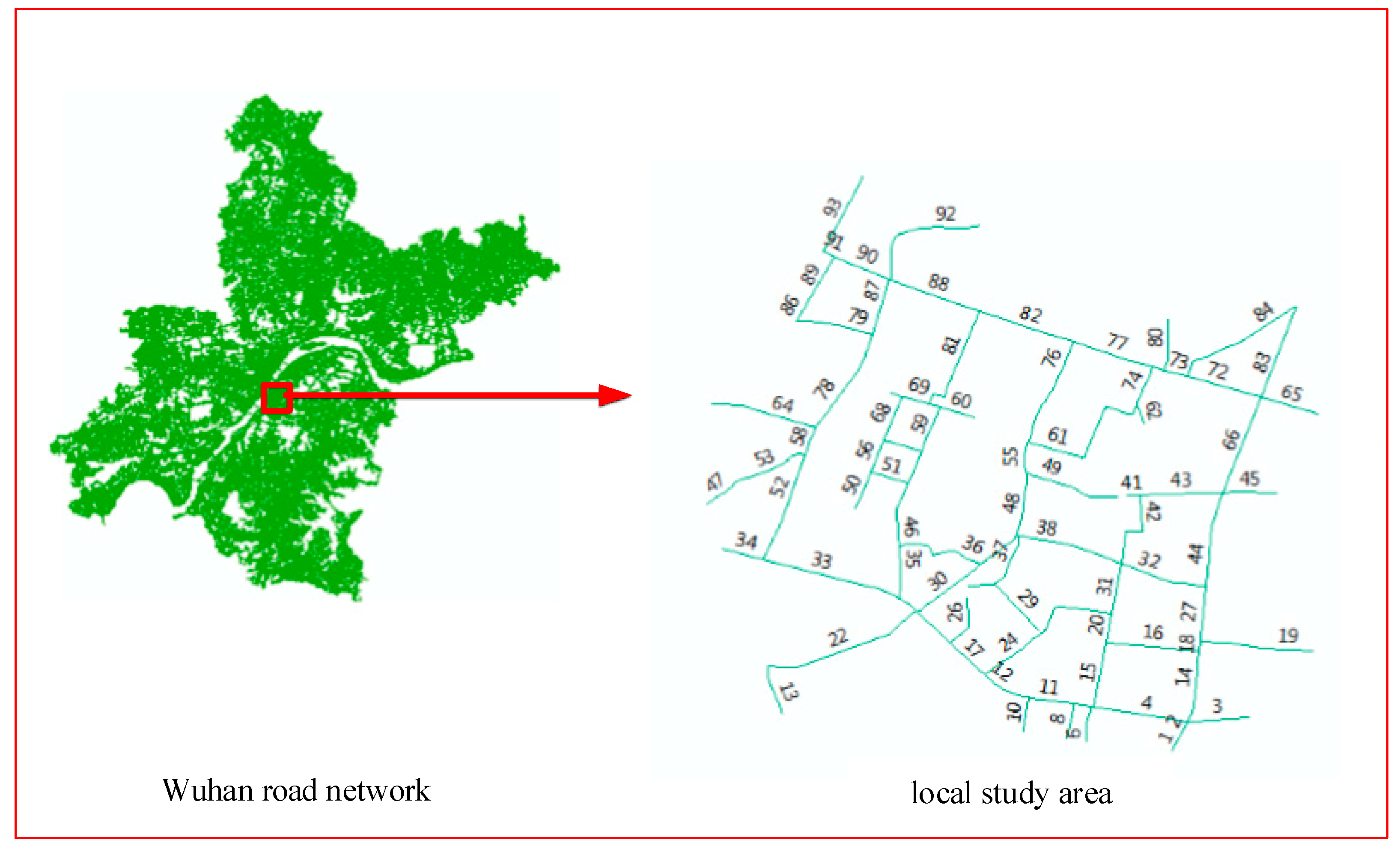
As shown in Figure 1, a link is defined as the segment between every two intersections of road network.
Definition 2.
Single vehicle link travel time is defined as the time a probe vehicle takes to traverse a target link from a beginning intersection to an ending intersection.
In our experiment, we choose one of the most commonly used indices, Pearson’s coefficient [1,16], to quantitatively measure the spatial and temporal correlations of travel time. The Pearson correlation coefficient, giving a value between −1 and +1, is used to measure the linear correlation between two variables x and y. It is developed by Karl Pearson and widely used in the sciences as a measure of the degree of linear dependence between two variables. Supposing two variables x and y, the Pearson’s correlation coefficient is defined as follows:
where and are the mean average of variables x and y, respectively. Similarly, and are corresponding standard deviations of variables x and y. Therefore, according to Equation (1), we can calculate the spatial correlation coefficient between target link and adjacent link.
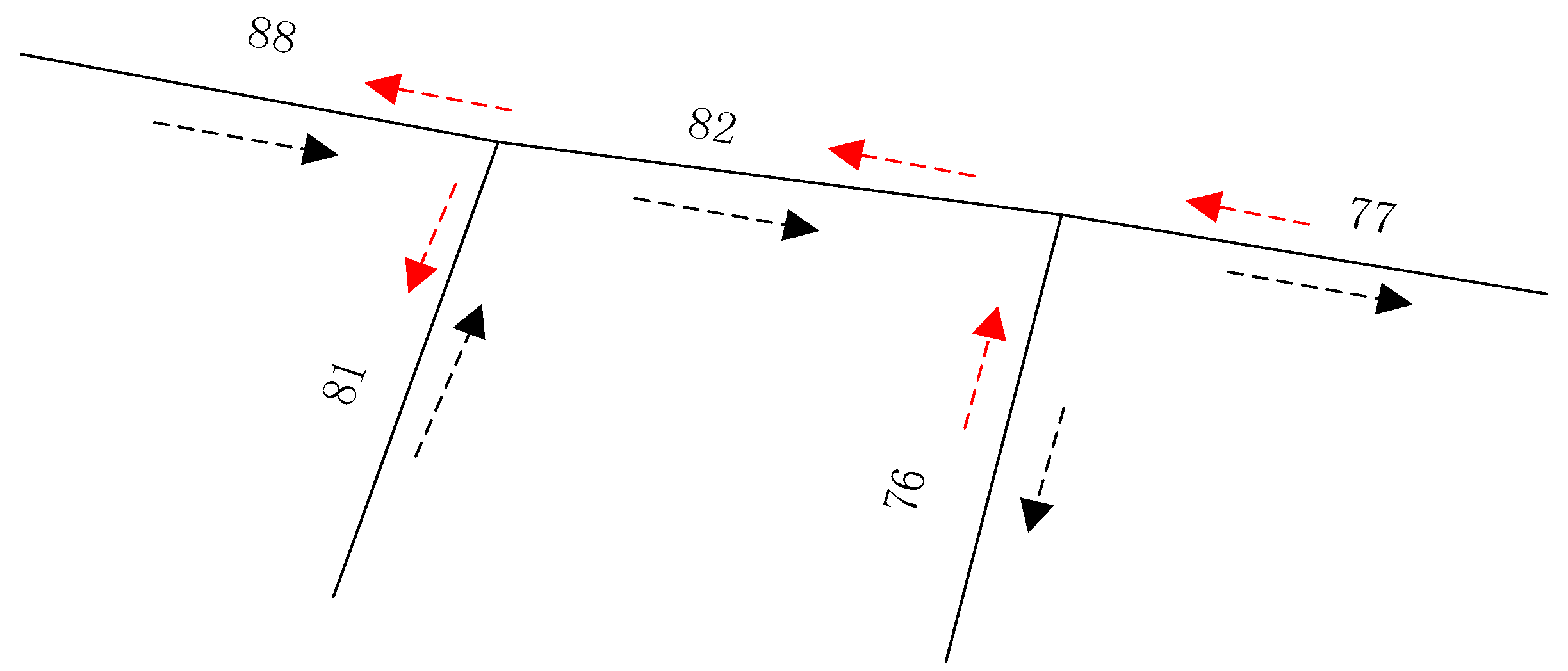
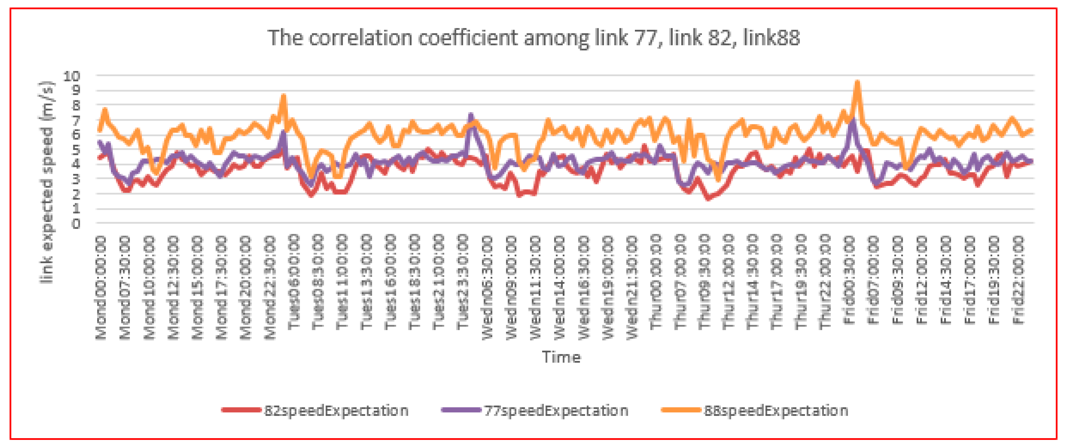
Figure 2 reveals schematic diagram of traffic flow, where link 88 is upstream link, link 82 is target link and link 77 is downstream link. As seen in Table 1, which shows the pair-wise correlations among link 82, link 77 and link 88, the correlation coefficient of speed expectation in a certain direction and different time are significantly correlated at 0.01 confidence level (two-tailed). Figure 3 is a line chart of the relationships for speed expectations among link 77, link 82 and adjacent link 88 from Monday to Friday. In Figure 3, the correlation coefficient of speed on different days presents different values and varies with day. The speed expectation of link 82 increases when the speed expectation of adjacent link 88 increases, presenting a positive correlation. We also see in Figure 3 that it displays a rhythmic pattern among the speed expectation of link 77, link 82 and link 88. Hence, both Table 1 and Figure 3 illustrate the dynamic spatial correlations among target links and adjacent links. Consequently, travel information of adjacent links was selected as model inputs to predict target link travel time.
3. Extracting Influencing Factors
Traffic flow is influenced by many factors such as traffic from adjacent areas, temperature, and rainfall. In this section, we extract influence factors from big historical traffic data and historical meteorological information to investigate their influence on link travel time prediction. Time, speed expectation, the standard deviation of speed, link degree, link length, and weather are closely related to traffic flow or road networks [7,17]. We extract these factors from big historical traffic data.
Existing research has shown that taxi trajectory trip patterns have weekly cycles [18,19]. The traffic flow of different direction is different and the same direction traffic flow between target and adjacent links has an important significance on each other. Figure 1 shows the local study area in the Wuhan road network. In this figure, the link number distinguishes different links. We extracted features of target link and adjacent link according to week’s cycle and traffic flow direction as depicted in Figure 2.
3.1. Traffic-Related Influencing Factors
Speed expectation and the standard deviation of speed are traffic-related characteristics that express the traffic of link. Some certain correlation between target link and adjacent link exists for these factors [7]. Consequently, we extracted features between a target link and adjacent links from quantities of statistical travel time information from taxis traversing the target link.
As shown in Figure 2, we extracted link traffic features in accordance with the direction of traffic flow. The traffic flow of black arrow direction of link 81 and link 88 has an effect on traffic flow of link 82 whose direction is black arrow direction too. The traffic flow of link 82 whose direction is black arrow direction also has influence on the traffic flow of link 77 and link 76 whose direction is also black arrow direction. At the same time, that the traffic flow is red arrow direction also influences each other. Therefore, we extracted speed expectation and speed standard deviation of link every 30 min according to the traffic flow direction. Subsequently, the calculation of traffic-related influence factors is as follows. Here, denotes link length, denotes travel time of the ith taxi traversing link, denotes average speed of the ith taxi traversing link, denotes speed expectation of taxi traversing link, and denotes speed standard deviation of taxi traversing link.
(1) Expectation of speed: .
We calculated average speed of single taxi traversing link according to Equation (2). As the travel time of every taxi traversing link is different, we computed the expected speed according to Equation (3) for every 30 min, representing the overall taxi travel speed.
(2) Standard deviation of speed: .
We calculated standard deviation of speed according to Equation (4) for every 30 min according to historical probe vehicle data, which reflects the variable speeds of different taxis traveling links over every 30 min.
Figure 3 is a line chart reflecting the relationship of expected speed among links 77, 82 and 88. As shown, the expected speed of link 82 increases when the expected speed of adjacent link 88 and link 77 increases, i.e. a positive correlation.
Figure 4 shows the variance in the standard deviation of speed over time among link 82, link 77 and link 88, respectively. As depicted in Figure 4, the standard deviation for speed decreases since taxis run at slower speeds during rush hours in mornings and evenings. A large variance occurs at other times of the day, when taxis travel with quite different speeds.
3.2. Ratio Relationship between Target Link and Adjacent Links
3.2.1. Link Degree Ratio between Target Link and Adjacent Links
Definition 3.
The degree of link connectivity is termed link degree, denoted by , and represents the sum of the links attached directly to the two endpoints of a link.
Connectivity degree of link, denoted by , is the sum of several links attached directly to the two endpoints of link. Link degree is one of the characteristics of road geometry. The greater the degree is, the more directly the link is connected. Therefore, the link guidance capacity of traffic is stronger. Degree ratio reflects the relationship of link between two links. We calculated degree ratio between target link and adjacent link in study region according to Equation (5) as neural network input information.
3.2.2. Length Ratio between Target Link and Adjacent Link
Generally, link travel time is mainly related with target link, such as the length of target link, and the speed of probe vehicle running in target link. At the same time, it is also affected by the adjacent link. Link length is also one of characteristics of road geometry. Generally, the greater the distance is, the longer is the travel time of a taxi traversing the link. The relationship of the link travel time between target link and adjacent link is expressed by the length ratio We calculated length ratio between target link and adjacent link in study region according to Equation (6) and used it as neural network input information.
3.2.3. Travel Time Ratio between Target Link and Adjacent Link
Link travel time reflects the traffic running state of a link but there is also a temporal relationship between a target link and an adjacent link; the travel time ratio of a target link and adjacent link. We calculated travel time ratio between a target link and adjacent links in the study region according to Equation (7) and this was used as output information of neural network to train the model.
3.3. Time Instant
Traffic states vary over the course of a day and between days of the week while link traffic has a weekly cycle [18,20,21], thus in our analysis we ignore differences between weeks and focus on the differences between days during a week. We assume that traffic flow remains consistent during every 30 min interval. Consequently, the day of the week and each 30 min interval during a day were regarded as neural network input information.
3.4. Weather Information
Among all meteorological factors, rainfall, air temperature, visibility, and wind are significantly relevant for understanding travel time. Snow and fog might increase the travel time for a driver from departure to arrival point. Therefore, we explore the effect of these factors on link travel time to improve prediction accuracy. A heavy rain waterlogs roadways, and makes the road surface slippery, thus traffic will be rather slow during and after rains. However, the traffic on sunny days is smoother. Heavy fog reduces visibility and might affect traffic. Hence, weather conditions must be considered when estimating and predicting travel time accurately.
Meteorological information was obtained from the public weather website http://tianqi.2345.com/wea_history/57494.htm and included date, day of week, minimum air temperature, maximum air temperature, weather, wind direction and wind force as depicted in Table 2. The weather information included visibility, and precipitation. However, there were no data for continuous wind direction or wind force in Wuhan City from April to July 2014. Meanwhile, annually, there is little fog and snow in Wuhan, and therefore it is unnecessary to consider the influence of wind, fog, and snow on link travel time estimation or prediction, in this instance. We just considered the influence of temperature and rainfall on traffic. Average air temperature and rainfall were chosen as inputs for the model, denoted by , respectively. Table 2 demonstrates meteorological information by day.
Based on this analysis, we designed an algorithm which extracted features or influence factors between target link and adjacent links. The travel time ratio between target link and adjacent links was regarded as output of model among all the extracted features and influence factors. Others were all regarded as inputs in our designed model. We conducted experiments using these extracted features and influencing factors.
4. The Artificial Neural Network Model
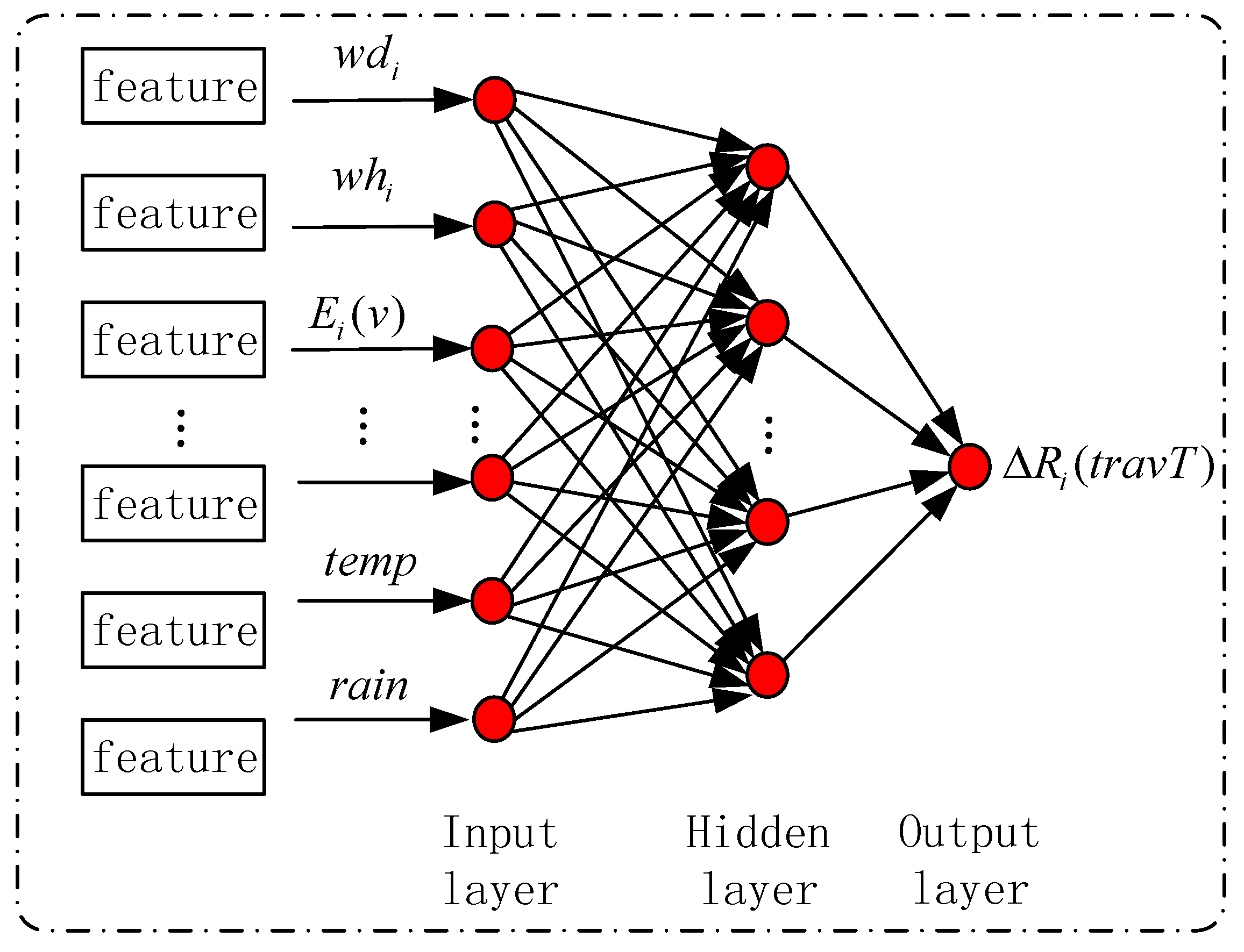
The Neural Network model [22,23] is a machine learning algorithm widely applied in traffic prediction. Although many ANNs could be applied in our framework, we chose a Back-propagation (BP) neural network with one hidden layer in the experiments for simplicity and generality. As discussed in Section 3, we chose eight features as input of ANN and one feature as output. The eight influence factors and one output are depicted and denoted as shown in Table 3. These are as follows: day of the week (), the 30 min during a day (), expected speed (), standard deviation of the speed (), degree ratio between target link and adjacent links (), length ratio between the target link and adjacent links (), temperature (temp), rainfall (rain), and travel time ratio between a target link and adjacent links (). As shown in Figure 5, we set eight neurons in the input layer and the number of neurons in output layer was set to one.
4.1. Input Layer
The input for this ANN was designed for an eight-dimension vector as depicted in Equation (8). It does not perform any calculation and just transmits signal to the next layer.
where denotes the ith vector of input layer. As depicted in Equation (8), denotes the day of the week and denotes the 30 min of the day. denotes the expected speed of adjacent link and denotes the standard deviation of speed on adjacent link. denotes the degree ratio between target link and adjacent link. denotes the length ratio between target link and adjacent link. temp denotes the average temperature corresponding to day and rain denotes the rainfall intensity corresponding time instant. All the features were calculated for each 30 min period.
4.2. Hidden Layer
Hidden layer is a standard layer of ANN that transfers the signal from the input layer to output layer. Its input is the output of layer, and its output is used as the input of the next layer. The calculation method of ANN in hidden layer is depicted as following equation.
where denotes the value of the nth hidden neuron, denotes the weight connecting the jth input neuron and the nth hidden neuron, denotes a bias with a fixed value for the nth hidden neuron, and denotes a transfer function.
4.3. Output Layer
This layer contains one neuron to generate the whole output of the neural network,
where denotes estimated travel time ratio of link, denotes the weight connecting the kth hidden neuron and the output neuron, and is the bias for the output.
5. Model Application
5.1. Data Description and Preparation
In our research, a private-sector company provided historical and real-time probe vehicle data for us to research travel time prediction. Probe vehicles collect information such as instantaneous speeds, timestamps, location, and azimuth, reflecting the running state of the urban traffic, and could play a crucial part in travel time estimation and prediction. The oracle database was acquired from ITS (Intelligent Traffic System) in Wuhan, China. We chose a partial road network in Wuhan city as a study area, as shown in Figure 1. The road network was bounded by Wuluo Road, Luoshi South Road, Xiongchu Avenue, and Dingziqiao Road, including many branches and paths. The road network was divided into links by crossing points where roads intersect. The degree of each link was obtained for the links in the entire network, except for links on the edge of the study area. Table 4 shows the selected local roads in the Wuhan road network, which includes the section number, geographic location and the length of each segment.
As a result of the effect of GPS positioning error [24], probe vehicles usually deviate from its actual driving road. Therefore, we first projected GPS points to those roads according to the probe vehicle trajectory with map-matching algorithm [15,25,26,27], and then, calculated link travel time using these corrected points. We calculated travel information including travel time, average speed of probe vehicles taking into consideration the probe vehicle running state at the intersections [28,29,30,31]. Table 5 depicts the travel characteristics extracted from the massive quantities of statistical travel time data, including obtained link ID, exiting endpoint ID, entering endpoint ID, probe vehicle ID, the travel time for a probe vehicle traversing the link, the moment a probe vehicle entered the link and the average speed of a probe vehicle traversing the link. Existing research has shown that probe vehicle trajectories display similar traffic patterns over a weekly cycle [18,21,32]. According to the weekly cycle of traffic, historical characteristics between target and upstream links were extracted. Figure 2 depicts road number and traffic direction on the partial road network shown in Figure 1. We used our model to predict travel times for link 82 considering spatiotemporal correlation among link 82, link 88, and link 77. Consequently, we extracted spatiotemporal correlation characteristics from big historical data from probe vehicles from May to July 2014—about three billion records.
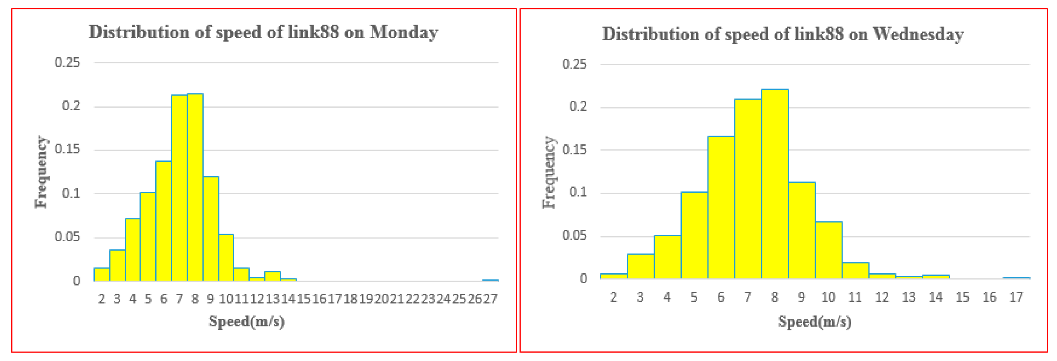
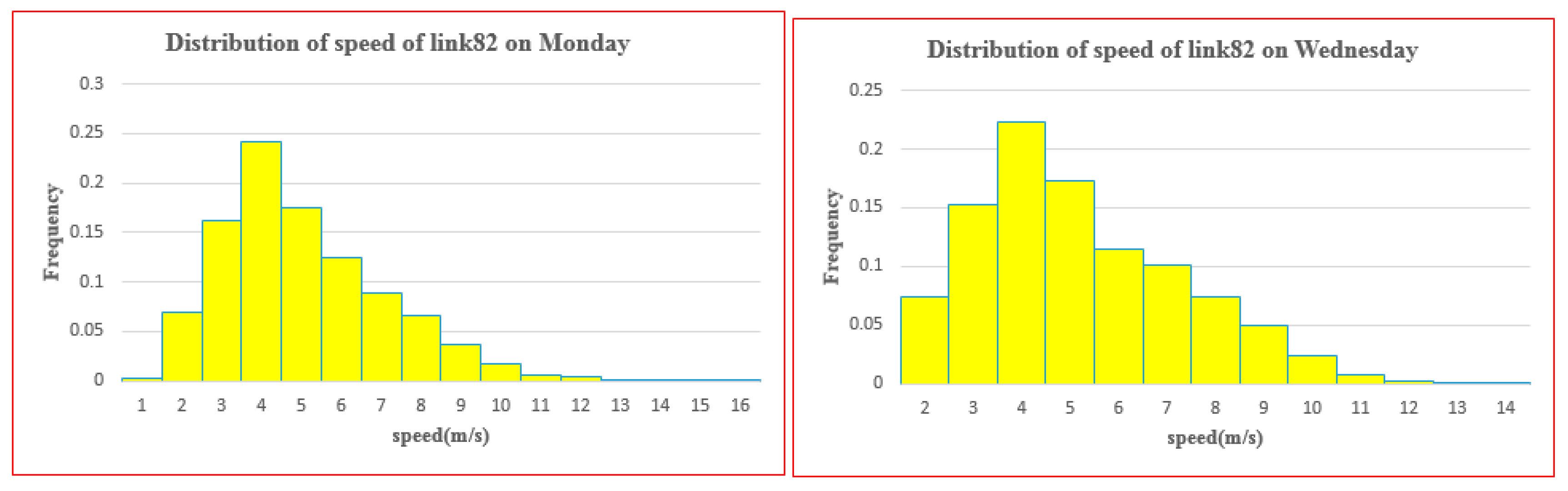
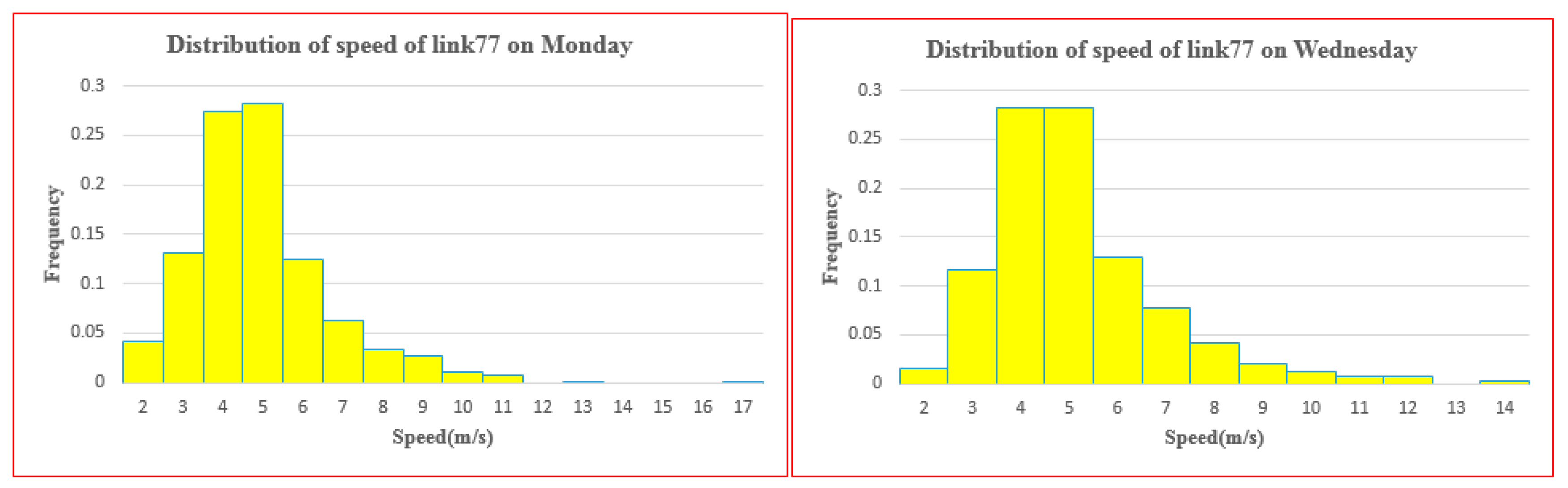
Table 6, Table 7 and Table 8 summarize historical big data, about 299,773,570 records from probe vehicle travel time information with descriptive statistics from January to May, 2014, including: mean value; standard deviation (SD); the 25th, 50th and 75th percentiles of travel time; and the minimum (Min), and maximum (Max) observations. Travel time data were recorded in the unit of seconds. From these three tables, it can be inferred that the quartile speed for the same link was similar for each day, with not much difference from day to day. In contrast, a great difference in speeds existed among different links. Figure 6, Figure 7 and Figure 8 show the distribution of speeds among the observations from link 88, link 82 and link 77 on Mondays and Wednesdays, respectively. A histogram of the same links presents a similar pattern, with an approximately normal distribution, if outliers are excluded. The distribution of travel speed however, shows slight differences among the different links.
We took link 82 for the sparse data link. Thus, link 82 and adjacent links including link 76, link 77, link 81 and link 88, were the research objects. To remove noisy data, statistical historical data were preprocessed. At the same time, historical data on workdays (from Monday to Friday, except holidays) were filtered as experimental data. Consequently, we calculated expected speed and the standard deviation for the speed of the adjacent links for every 30 min period from preprocessed historical data according to the weekly cycle and traffic flow direction as depicted in Figure 2. The features were calculated according to Section 3 and shown in Table 9. The travel time of adjacent links is the key point when predicting target link travel time as this value reflects the localized state of traffic overall. Finally, we extracted 2078 features as input for the neural network and 2078 features as output corresponding to input features. Of all the extracted features, a portion of these features was taken as training data for the ANN model. Another different portion of these features was taken as test data to verify the validity of the model.
Partial meteorological information was selected to research their influence on link travel time prediction. As for the meteorological information, we only considered the influence of temperature and rainfall on traffic based on our previous analysis discussed in Section 3.4. We defined degree of rainfall into four ranks according to historical rainfall: rainless, drizzle, downpour and thunder, corresponding to the digital values 1, 2, 3 and 4, respectively. The input and output information of our model are depicted in Table 9.
5.2. Neural Network Training
A training process is necessary before the ANN model can be applied to estimate link travel times. In our proposed model, the Levenberg–Marquardt algorithm was chosen for neural network training as it provides fast convergence even for large networks. The learning rate was set to 0.01 to maintain the stability of neural network. The gradient was set to 1 × 10⁻⁵ and the number of validation checks was set to ten. Three procedures including training, validation, and testing were conducted during the entire training process.
As depicted in Table 10, we divided the whole dataset into three subsets; the training dataset, validation dataset, and testing dataset. Different quantities of data were used for training, validation and testing, respectively. The amount of validation remains the same, namely 10% of total data, the training data were 89%, 85%, 80% and 70%, respectively. In addition, the corresponding testing data were 1%, 5%, 10% and 20%. The training dataset was used in neural network for training, while the validation dataset was used to stop training when the network performance on the validation dataset failed to improve or remained the same. The validation dataset was used to prevent over-fitting and ensures the generalizability of results from the network. The testing dataset was used to test the performance of trained neural network and acted as a further check on results. Testing had no effect on training. After training and validation, the trained ANN model was applied to predict link travel times for links at different time instants.
5.3. Model Evaluation
In this section, two performance indicators were used to evaluate the performance of our neural network model. As two of the most commonly used indicators, and for their simplicity and representativeness, we chose Root Mean Square Error (RMSE) and Mean Absolute Percentage Error (MAPE) to be indicators:
where denotes the estimated travel time of probe vehicle traveling target link, and is true link travel time.
5.4. Results of ANN Based on Real GPS Data
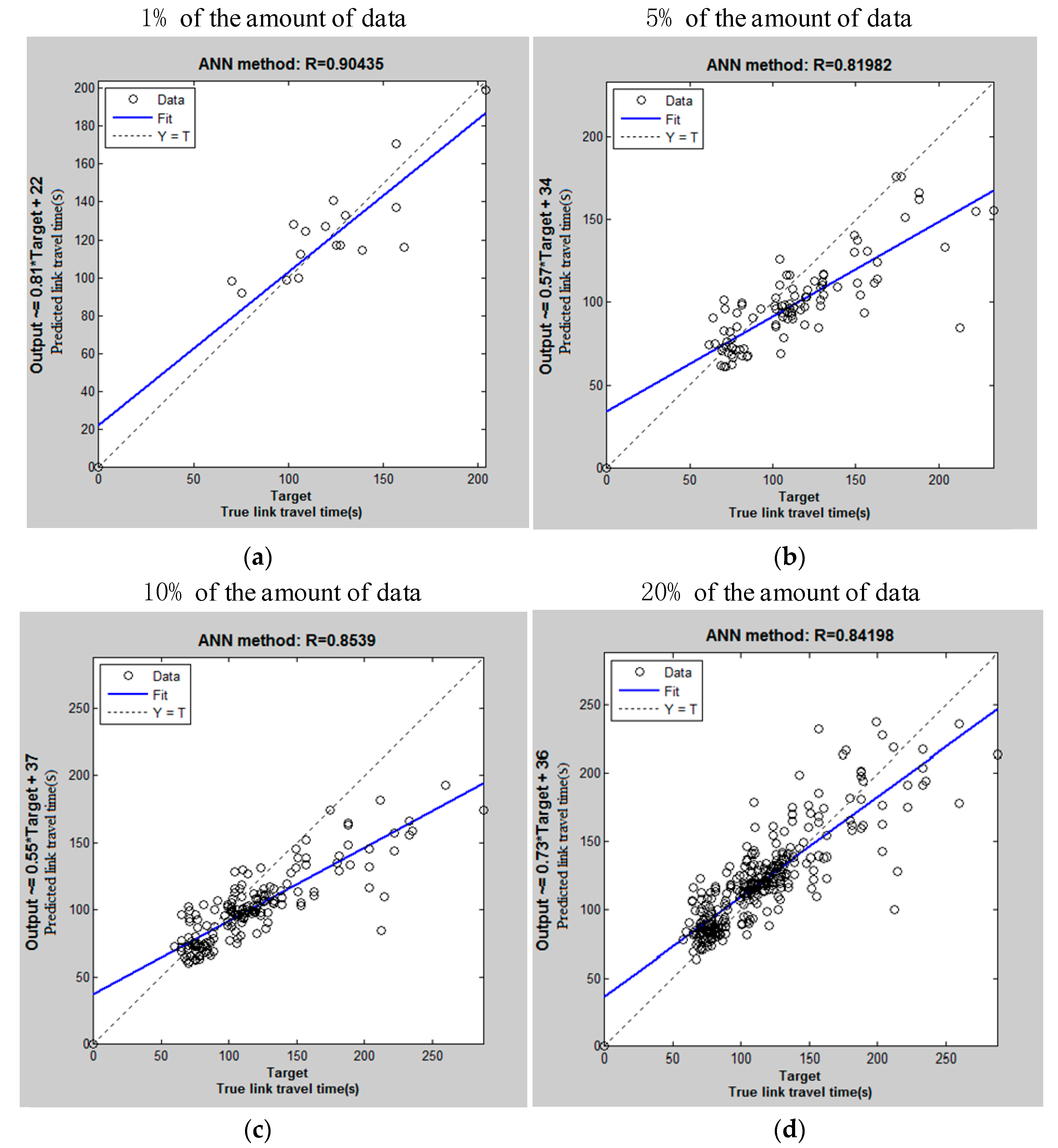
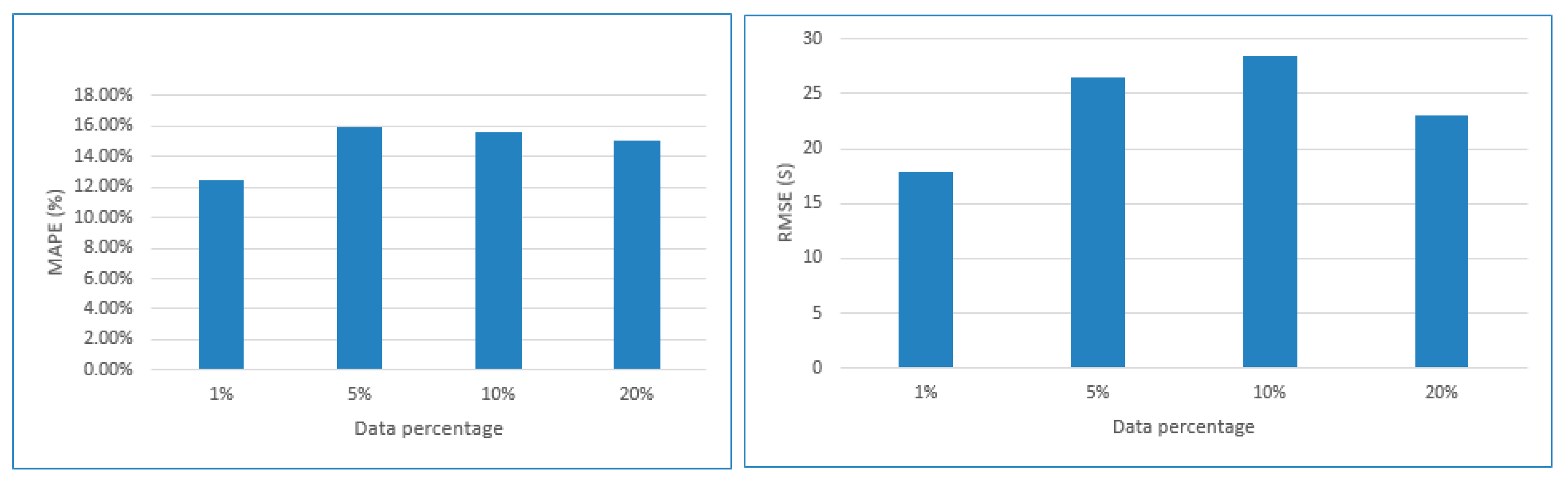
In our experiment, the trained model obtained according to extracted historical features was used to predict link travel time based on real GPS data and different datasets were used to verify our proposed model. As depicted in Figure 9, the correlation between true link travel time and predicted link travel time corresponded to different testing datasets. The horizontal axis represents true link travel time while the vertical axis denotes predicted link travel time. The linear correlation coefficient R value indicates the correlation between true link travel time and predicted link travel time. As we can see in Figure 9, with an increasing quantity of data, the R value trended downward. Table 10 shows the prediction accuracy corresponding to different testing data. The value of MAPE becomes slightly bigger with an increase in the amount of data from 1 to 5% of the total data. As shown in Figure 9a, it reaches the best prediction effect from the perspective of MAPE when the data were 1% of the total data. The mean absolute percentage error was 12.46% and the root mean square error was 17.96 s. However, the MAPE values corresponding to different testing data obtained values closer to each other when the testing data were 5%, 10% and 20%, as shown in Figure 10: 15.90%, 15.61%, and 15.02%, respectively.
5.5. Sensitivity Analysis of Different Influencing Factors
We constructed different ANN models to understand factors influencing link travel time, such as weather, and temperature. As mentioned in Section 3, the input features of neural network model includes day of the week (), which 30 min of the day (), expected speed (), standard deviation of speed (), degree ratio between target link and adjacent link (), length ratio between target link and adjacent link (), temperature (temp) and rainfall (rain). The output of ANN models was the travel time ratio between target link and adjacent link (). The role each feature plays in predicting travel time in the neural network model needed to be verified. Therefore, different models were constructed with different factors and the sensitivity of factors on travel time prediction was analyzed. We constructed different neural network models by combining input features and used the average absolute percentage error (MAPE) to measure the performance of these ANN models. To construct models conveniently, we use simple variable F1 to F8 as depicted in Table 3 to denote the input features of different models and constructed them as follows.
(1) Model M: including all input features
This model includes all input features and it is regard as a benchmark compared with other models. The input feature of Model M includes F1, F2, F3, F4, F5, F6, F7 and F8.
(2) Model A: without day of the week
Time information reflects the travel characteristic of probe vehicle during different time periods. The day of the week distinguishes different travel times corresponding to different days in a week. The ANN model without day of the week was trained as Model A. The input features of Model A included F2, F3, F4, F5, F6, F7 and F8.
(3) Model B: without 30 min time interval of the day
The 30 min intervals of the day distinguish different travel times corresponding to different time periods. The ANN model excluding 30 min of a day was trained as Model B. The input feature of Model B includes F1, F3, F4, F5, F6, F7 and F8.
(4) Model C: without expected speed
The expected speed reflects the state of traffic on a road. The ANN model without expected speed was trained as Model C. The input feature of Model C includes F1, F2, F4, F5, F6, F7 and F8.
(5) Model D: without the standard deviation of speed
The standard deviation of speed reflects the variance in speeds on a link. The ANN model without the standard deviation of speed was trained as Model D. The input feature of Model D includes F1, F2, F3, F5, F6, F7 and F8.
(6) Model E: without length ratio
The ANN model without length ratio was trained as Model E. The input feature of Model E includes F1, F2, F3, F4, F6, F7 and F8.
(7) Model F: without degree ratio
The ANN model without degree ratio was trained as Model F. The input feature of Model F includes F1, F2, F3, F4, F5, F7 and F8.
(8) Model G: without temperature
The ANN model without temperature was trained as Model G. The input feature of Model G includes F1, F2, F3, F4, F5, F6 and F8.
(9) Model H: without rain
The ANN model without rain was trained as Model H. The input feature of Model H includes F1, F2, F3, F4, F5, F6 and F7.
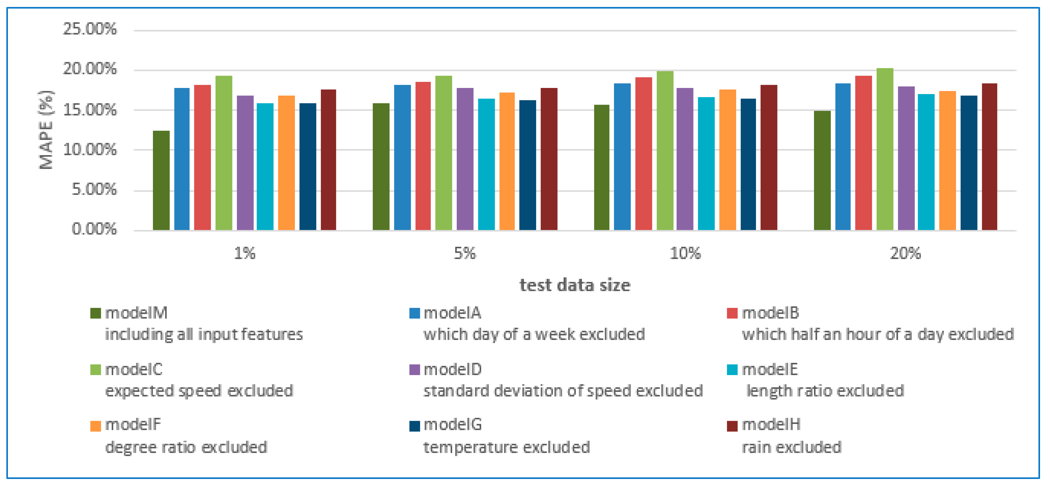
In the comparison experiment, we used the same dataset to train different ANN models and the same dataset was used to test those trained models using MAPE. Consequently, we conducted experiments using the same training dataset and four groups of testing dataset for each trained model to test the trained model. It can reflect the influence of model constituted by different factors on link travel time prediction. As shown in Table 11, it quantifies the influence of different factors. In general, model M has smaller MAPE than other models. Figure 11 illustrates the influence of different models on the performance of ANNs under the condition of different testing dataset. As shown in Figure 11, different factors influence the prediction of link travel time. Model M had greater prediction accuracy overall, as the MAPE value was lower. Models with the three factors day of the week, 30 min period of the day, and the expected speed of adjacent link influenced link travel time prediction had a higher value of MAPE than those models without them. The expected speed of an adjacent link had the greatest effect on link travel time prediction among those three factors; the biggest MAPE value appeared in the model excluding expected speed in link travel time prediction. The degree ratio and temperature slightly influence link travel time prediction. Rainfall affects link travel time prediction but is not as important as time of day as expressed by 30 min interval, expected speed of adjacent links, or day of the week. The MAPE value was smaller when rainfall was excluded from the model, as shown in the sensitivity analysis seen in Figure 11.
6. Discussion and Conclusions
Previous studies have focused on analyzing raw data from GPS sensors to promote the accuracy of GPS data. Recent research has focused on developing methods to study link travel time prediction, such as the Kalman filter model and other data driven models. Generally, the existing methods can best predict link travel times when there are abundant data. However, they ignore situations when there are insufficient data and do not account for meteorological factors. Consequently, to predict link travel time using sparse data, incorporating multi-factors is a challenge.
We propose an ANN model for travel time prediction of target links using sparse data and incorporating the influence of multi-factors such as weather conditions. The running state of probe vehicle to some extent reflects the state of road traffic. Using data collected by probe vehicles, we aggregated data from Monday to Friday for single taxis traveling target link on weekdays. We extracted feature relationships between target links and adjacent links for time-periods based on big data from probe vehicles. Temperature and rainfall were also input to our ANN model. We designed a three-layer artificial neural network model with eight neurons in the input layer and one neuron in the output layer. Of all these extracted features, the ratio between target link and adjacent link was the output of ANN model and the other features were the input of ANN model. We used the designed artificial neural network model for training, validation. Finally, the trained neural network model was used for link travel time prediction. Different models constructed with different factors were used to evaluate the influence of factors on link travel time prediction. The main contribution of our research is that we can predict link travel time using sparse data. At the same time, we incorporated multi-factors into our model and researched their influence on link travel time. The model was verified by historical big data—about 224,830,178 records from probe vehicles from May to July 2014. The experimental results showed that, when data are sparse, we can obtain better results using an artificial neural network model based on feature relationships between target links and adjacent links and big historical data. We could know from model comparison, all those factors we selected have influence on link travel time prediction. Among those factors, the three factors the day of the week, the 30 min interval of the day, and the expected speed of adjacent links had higher influence on link travel time prediction than other factors Rainfall also affected link travel time prediction but is not as important as the three dominant factors.
Our results are influenced by techniques and experimental conditions. For example, the location accuracy is influenced by GPS devices, while the map-matching algorithm affects the precision of GPS trajectories. Meanwhile, travel time is also affected by the calculation algorithms for single probe vehicles traveling target links. This paper only focused on link travel time on a local road network. In the future, we will validate this model using links in other areas of the Wuhan road network, the road networks in other Chinese cities, and using larger real datasets. We will further validate the ANN model considering other factors which might be relevant in Chinese cities, such as the number of lanes, snow, and wind conditions. We will also apply this model to predict route travel time based on probe vehicle data.
Acknowledgments
This work was supported by National Natural Science Foundation of China No. 41271401; the National 863 project, Multi-source Information Real-time Access and Heterogeneous Information Autonomous Loading Technology under the Unified Spatiotemporal System, No. 2013AA122301; Pan-information map fusion technology Based on the Internet superposition protocol, No. 2013AA12A203; National Science and Technology Support Plan, the Key Technology and Applications of Location-based Sensor Network and Pan-information Map, No. 2012BAH35B03; and National Science Foundation, Nos. 1416509, ACI-1535031,and 1535081; National Key R&D Program of China (Grant No.2016YFB0502204), and Opening research fund of State Key Laboratory of Information Engineering in Surveying, Mapping and Remote Sensing. Finally, the authors thank Steve for his proofreading.
Author Contributions
Faming Zhang performed the research, analyzed the data and wrote the paper. Xinyan Zhu co-designed the research. Yaxin Fan developed some earlier prototypes. Xinyue Ye co-designed the research and extensively updated the paper. Chen Chen and Han Yue edited the paper. All authors read and approved the final manuscript.
Conflicts of Interest
The authors declare no conflict of interest.
References
- Liu, K.; Yamamoto, T.; Morikawa, T. Feasibility of using taxi dispatch system as probes for collecting traffic information. J. Intell. Transp. Syst. Technol. Plan. Oper. 2009, 13, 16–27. [Google Scholar] [CrossRef]
- Oh, J.S.; Jayakrishnan, R.; Recker, W. Section travel time estimation from point detection data. In Proceedings of the 82nd Annual Meeting of Transportation Research Board, Washington, DC, USA, 12–16 January 2003. [Google Scholar]
- Van Lint, J.W.C.; Van Der Zijpp, J. Improving a travel time estimation algorithm by using dual loop detectors. Transp. Res. Rec. J. Transp. Res. Board 2003, 1855, 41–48. [Google Scholar] [CrossRef]
- Kwon, J.; Petty, K. A travel time prediction algorithm scalable to freeway networks with many nodes with arbitrary travel routes. In Proceedings of the TRB 84th Annual Meeting, Washington, DC, USA, 9–13 January 2005. [Google Scholar]
- Liu, H.; Van Zuylen, H.J.; Van Lint, J.W.C.; Salomons, M. Urban arterial travel time prediction with state-space neural networks and Kalman filters. Transp. Res. Rec. J. Transp. Res. Board 2006, 1968, 99–108. [Google Scholar] [CrossRef]
- Jula, H.; Dessouky, M.; Ioannou, P.A. Real-time estimation of travel times along the arcs and arrival times at the nodes of dynamic stochastic networks. IEEE Trans. Intell. Transp. Syst. 2008, 9, 97–110. [Google Scholar] [CrossRef]
- Zheng, Y.; Liu, F.; Hsieh, H.P. U-Air: When urban air quality inference meets big data. In Proceedings of the ACM 19th ACM SIGKDD International Conference on Knowledge Discovery and Data Mining, Chicago, IL, USA, 11–14 August 2013; ACM: New York, NY, USA, 2013; pp. 1436–1444. [Google Scholar]
- Hellinga, B.; Izadpanah, P.; Takada, H.; Fu, L. Decomposing travel times measured by probe-based traffic monitoring systems to individual road segments. Transp. Res. Part C Emerg. Technol. 2008, 16, 768–782. [Google Scholar] [CrossRef]
- Jenelius, E.; Koutsopoulos, H.N. Travel time estimation for urban road networks using low frequency probe vehicle data. Transp. Res. Part B Methodol. 2013, 53, 64–81. [Google Scholar] [CrossRef]
- Zhan, X.; Hasan, S.; Ukkusuri, S.V.; Kamga, C. Urban link travel time estimation using large-scale taxi data with partial information. Transp. Res. Part C Emerg. Technol. 2013, 33, 37–49. [Google Scholar] [CrossRef]
- Zheng, Y.; Liu, Y.; Yuan, J.; Xie, X. Urban computing with taxicabs. In Proceedings of the ACM 13th International Conference on Ubiquitous Computing, Beijing, China, 17–21 September 2011; ACM: New York, NY, USA, 2011; pp. 89–98. [Google Scholar]
- Herring, R.; Hofleitner, A.; Abbeel, P.; Bayen, A. Estimating arterial traffic conditions using sparse probe data. In Proceedings of the 2010 13th International IEEE Conference on Intelligent Transportation Systems (ITSC), Funchal, Portugal, 19–22 September 2010; IEEE: Piscataway Township, NJ, USA, 2010; pp. 929–936. [Google Scholar]
- Wang, Y.; Zheng, Y.; Xue, Y. Travel time estimation of a path using sparse trajectories. In Proceedings of the ACM 20th ACM SIGKDD International Conference on Knowledge Discovery and Data Mining, New York, NY, USA, 24–27 August 2014; ACM: New York, NY, USA, 2014; pp. 25–34. [Google Scholar]
- Yao, E.J.; Zuo, T. Real-time map matching algorithm based on low-sampling-rate probe vehicle data. J. Beijing Univ. Technol. 2013, 39, 909–913. [Google Scholar]
- Zhang, Y.; Yang, B.; Luan, X. Automated matching urban road networks using probabilistic relaxation. Acta Geod. Catogr. Sin. 2012, 41, 933–939. [Google Scholar]
- Soper, H.E.; Young, A.W.; Cave, B.M.; Lee, A.; Pearson, K. On the distribution of the correlation coefficient in small samples. Appendix II to the papers of “Student” and R. A. Fisher. A cooperative study. Biometrika 1917, 11, 328–413. [Google Scholar] [CrossRef]
- Rantala, J.; Culley, J. Analysis of Relationships between Road Traffic Volumes and Weather: Exploring Spatial Variation. In Proceedings of the 2014 EDBT/ICDT Workshops, Athens, Greece, 28 March 2014. [Google Scholar]
- Fei, X.; Lu, C.C.; Liu, K. A bayesian dynamic linear model approach for real-time short-term freeway travel time prediction. Transp. Res. Part C Emerg. Technol. 2011, 19, 1306–1318. [Google Scholar] [CrossRef]
- Fang, Z.; Li, Q.; Shaw, S.L. What about people in pedestrian navigation? Geo-Spat. Inf. Sci. 2015, 18, 135–150. [Google Scholar] [CrossRef]
- Zhang, F.; Zhu, X.; Guo, W.; Ye, X.; Hu, T.; Huang, L. Analyzing Urban Human Mobility Patterns through a Thematic Model at a Finer Scale. ISPRS Int. J. Geo-Inf. 2016, 5, 78. [Google Scholar] [CrossRef]
- Liu, X.; Gong, L.; Gong, Y.; Liu, Y. Revealing daily travel patterns and city structure with taxi trip data. arXiv, 2013; arXiv:1310.6592. [Google Scholar]
- Wei, Y.; Chen, M.-C. Forecasting the short-term metro passenger flow with empirical mode decomposition and neural networks. Transp. Res. Part C Emerg. Technol. 2012, 21, 148–162. [Google Scholar] [CrossRef]
- Van Hinsbergen, C.; van Lint, J.; van Zuylen, H. Bayesian committee of neural networks to predict travel times with confidence intervals. Transp. Res. Part C Emerg. Technol. 2009, 17, 498–509. [Google Scholar] [CrossRef]
- Zuo, C. Ontology-Based Modeling, Annotation, Storage, and Query of Semantic Trajectories for Travel Analysis. Ph.D. Thesis, East China Normal University, Shanghai, China, 2011. [Google Scholar]
- Chen, B.Y.; Yuan, H.; Li, Q.; Lam, W.H.; Shaw, S.L.; Yan, K. Map-matching algorithm for large-scale low-frequency floating car data. Int. J. Geogr. Inf. Sci. 2014, 28, 22–38. [Google Scholar] [CrossRef]
- Yuan, J.; Zheng, Y.; Zhang, C.; Xie, X.; Sun, G.Z. An interactive-voting based map matching algorithm. In Proceedings of the 2010 Eleventh International Conference on Mobile Data Management, Kansas City, MO, USA, 23–26 May 2010; IEEE Computer Society: Washington, DC, USA, 2010; pp. 43–52. [Google Scholar]
- Li, Q.; Bo, H.; Yang, Y. Flowing car data map-matching based on constrained shortest path algorithm. Geomat. Inf. Sci. Wuhan Univ. 2013, 38, 805–808. [Google Scholar]
- Yu, D.X.; Gao, X.Y.; Yang, Z.S. Individual vehicle travel time estimation based on GPS data and analysis of vehicle running characteristics. J. Jilin Univ. Eng. Technol. Ed. 2010, 40, 965–970. [Google Scholar]
- Dong, H.; Wu, F. Estimation of Average Link Travel time Using Fuzzy C-Mean. Bull. Sci. Technol. 2011, 27, 426–430. [Google Scholar]
- Liu, H. A virtual vehicle probe model for time-dependent travel time estimation on signalized arterials. Transp. Res. Part C Emerg. Technol. 2009, 17, 11–26. [Google Scholar] [CrossRef]
- Jiang, G.; Chang, A.; Zhang, W. Comparison of link travel time estimation methods based on GPS equipped floating car. J. Jilin Univ. Eng. Technol. Ed. 2009, 39, 182–186. [Google Scholar]
- Zhang, F.; Zhu, X.; Hu, T.; Guo, W.; Chen, C.; Liu, L. Urban Link Travel Time Prediction Based on a Gradient Boosting Method Considering Spatiotemporal Correlations. ISPRS Int. J. Geo-Inf. 2016, 5, 201. [Google Scholar] [CrossRef]
Figure 1.
Visualization of the local road network in Wuhan City, China.

Figure 2.
Schematic diagram of traffic flow. Red line represents traffic flow in one direction and black line are opposite.
Figure 2.
Schematic diagram of traffic flow. Red line represents traffic flow in one direction and black line are opposite.

Figure 3.
The correlation among link 77, link 82 and link 88.

Figure 4.
Line chart of speed standard deviation among link 77, link 82, and link 88.

Figure 5.
Model structure of BP neural network. , day of the week; , the 30 min during a day; , expected speed; temp, temperature; rain, rainfall; , travel time ratio between a target link and adjacent links. Arrows in this figure represent input data flow and red points stand for neurons in neural network.

Figure 6.
Distribution of speeds among the observations of link 88 on Monday and Wednesday.

Figure 7.
Distribution of speeds among the observations of link 82 on Monday and Wednesday.

Figure 8.
Distribution of speeds among the observations of link 77 on Monday and Wednesday.

Figure 9.
Correlation of link 82 between true link travel time and estimated link travel time.

Figure 10.
The Mean Absolute Percentage Error (MAPE) and Root Mean Square Error (RMSE) of predicted link travel time corresponding to different data percentage.
Figure 10.
The Mean Absolute Percentage Error (MAPE) and Root Mean Square Error (RMSE) of predicted link travel time corresponding to different data percentage.

Figure 11.
Influence of different input factors on ANN model.


Table 1.
The correlation coefficient of speed expectation in a certain direction and different time among target link 82, adjacent link 77 and adjacent link 88.
Table 1.
The correlation coefficient of speed expectation in a certain direction and different time among target link 82, adjacent link 77 and adjacent link 88.
| Link | Monday | Tuesday | Wednesday | Thursday | Friday |
|---|---|---|---|---|---|
| Link 77, link 82 in −1 traffic flow direction | 0.755327 ** | 0.599857 ** | 0.451914 ** | 0.575618 ** | 0.558733 ** |
| Link 88, link 82 in −1 traffic flow direction | 0.719256 ** | 0.837093 ** | 0.762925 ** | 0.715509 ** | 0.605603 ** |
** Significantly correlated at 0.01 confidence level (two-tailed).
Table 2.
Meteorological information by day.
| Date | Weekday | Minimum Air Temperature (°C) | Maximum Air Temperature (°C) | Weather | Wind Direction | Wind Force |
|---|---|---|---|---|---|---|
| 4 May 2014 | Sunday | 11 | 21 | light rain to cloudy | No | No |
| 7 May 2014 | Wednesday | 17 | 28 | clear to overcast cloudy | No | No |
| 24 May 2014 | Saturday | 20 | 27 | light rain to heavy rain | No | No |
Table 3.
Input features and corresponding output feature.
| 1 | 2 | 3 | 4 | 5 | 6 | 7 | 8 | 9 |
|---|---|---|---|---|---|---|---|---|
| temp | rain | |||||||
| F1 | F2 | F3 | F4 | F5 | F6 | F7 | F8 | F9 |
Table 4.
Selected arterial road network used in the experiment.
| Section ID | Start Coordinate | End Coordinate | Length (Meter) | ||
|---|---|---|---|---|---|
| Latitude | Longitude | Latitude | Longitude | ||
| 88 | 30.535 | 114.329 | 30.533 | 114.334 | 475.69 |
| 82 | 30.533 | 114.334 | 30.532 | 114.338 | 489.10 |
| 77 | 30.532 | 114.338 | 30.530 | 114.342 | 411.43 |
Table 5.
Travel information from individual probe vehicles.
| Link ID | Enter Endpoint ID | Exit Endpoint ID | Probe Vehicle ID | Time Instant | Travel Time (s) | Average Speed (m/s) |
|---|---|---|---|---|---|---|
| 82 | 35 | 48 | 23501 | 3 June 2014 03:17:11 | 100.0 | 4.89 |
| 82 | 35 | 48 | 22608 | 2 June 2014 00:00:50 | 85.0 | 5.75 |
| 82 | 48 | 35 | 29444 | 2 June 2014 00:12:03 | 101.0 | 4.84 |
Table 6.
Basic statistics of travel speed (m/s) about link 88 1.
| Workday | Mean | SD | 25th | 50th | 75th | Min | Max |
|---|---|---|---|---|---|---|---|
| Monday | 6.55 | 2.22 | 5.23 | 6.61 | 7.8 | 1.03 | 26.43 |
| Tuesday | 6.56 | 2.19 | 5.17 | 6.61 | 7.8 | 1.15 | 15.35 |
| Wednesday | 6.64 | 1.95 | 5.41 | 6.61 | 7.8 | 1.46 | 16.4 |
| Thursday | 6.68 | 2.23 | 5.52 | 6.7 | 7.8 | 1.43 | 18.3 |
| Friday | 6.42 | 2.10 | 5.23 | 6.34 | 7.55 | 1.2 | 15.86 |
1 SD, standard deviation.
Table 7.
Basic statistics of travel speed (m/s) for link 82.
| Workday | Mean | SD | 25th | 50th | 75th | Min | Max |
|---|---|---|---|---|---|---|---|
| Monday | 4.83 | 2.15 | 3.27 | 4.33 | 6.04 | 0.94 | 15.78 |
| Tuesday | 4.82 | 2.08 | 3.26 | 4.41 | 6.09 | 1.06 | 13.97 |
| Wednesday | 4.73 | 2.09 | 3.12 | 4.25 | 6.19 | 1.04 | 13.59 |
| Thursday | 4.77 | 2.18 | 3.14 | 4.33 | 6.25 | 0.93 | 13.22 |
| Friday | 4.97 | 2.20 | 3.37 | 4.61 | 6.04 | 1.11 | 17.47 |
Table 8.
Basic statistics of travel speed (m/s) about link 77.
| Workday | Mean | SD | 25th | 50th | 75th | Min | Max |
|---|---|---|---|---|---|---|---|
| Monday | 4.42 | 1.77 | 3.27 | 4.16 | 5.08 | 1.2 | 16.46 |
| Tuesday | 4.16 | 1.61 | 3.21 | 3.92 | 4.84 | 1.12 | 13.72 |
| Wednesday | 4.61 | 1.81 | 3.37 | 4.29 | 5.14 | 1.32 | 13.72 |
| Thursday | 4.18 | 1.52 | 3.14 | 4.03 | 4.84 | 1.04 | 11.76 |
| Friday | 4.47 | 1.82 | 3.37 | 4.24 | 5.02 | 1.24 | 18.7 |
Table 9.
Example of the training and testing dataset (inputs and output of artificial neural network (ANN) model).
Table 9.
Example of the training and testing dataset (inputs and output of artificial neural network (ANN) model).
| 1 | 2 | 3 | 4 | 5 | 6 | 7 | 8 | 9 |
|---|---|---|---|---|---|---|---|---|
| temp | rain | |||||||
| F1 | F2 | F3 | F4 | F5 | F6 | F7 | F8 | F9 |
| 1 | 0.1 | 5.32 | 1.97 | 1 | 0.7984 | 25.25 | 1 | 0.7374 |
| 2 | 0.1 | 5.58 | 1.79 | 1 | 0.7984 | 28.78 | 1 | 0.714 |
| 5 | 3.3 | 2.55 | 0.96 | 0.8 | 1.0282 | 26.36 | 2 | 0.4355 |
| 3 | 3.4 | 5.02 | 1.02 | 1.3333 | 1.0529 | 28.34 | 1 | 2.0021 |
Table 10.
Training, evaluation and testing dataset 1.
| Total Data | Training (Percentage) | Validation (Percentage) | Testing (Percentage) | RMSE | MAPE |
|---|---|---|---|---|---|
| 2078 | 1849 (89%) | 208 (10%) | 20 (1%) | 17.9606 | 12.46% |
| 1766 (85%) | 208 (10%) | 104 (5%) | 26.5225 | 15.90% | |
| 1662 (80%) | 208 (10%) | 208 (10%) | 28.4815 | 15.61% | |
| 1454 (70%) | 208 (10%) | 417 (20%) | 23.0553 | 15.02% |
1 RMSE, Root Mean Square Error; MAPE, Mean Absolute Percentage Error.
Table 11.
MAPE of ANN with some influence factors excluded.
| Testing Dataset | Model M | Model A | Model B | Model C | Model D | Model E | Model F | Model G | Model H |
|---|---|---|---|---|---|---|---|---|---|
| 1% | 12.46% | 17.85% | 18.08% | 19.28% | 16.86% | 15.79% | 16.84% | 15.97% | 17.54% |
| 5% | 15.90% | 18.23% | 18.56% | 19.33% | 17.73% | 16.38% | 17.17% | 16.17% | 17.78% |
| 10% | 15.61% | 18.27% | 19.19% | 19.88% | 17.79% | 16.65% | 17.59% | 16.45% | 18.21% |
| 20% | 15.02% | 18.43% | 19.27% | 20.21% | 17.97% | 17.07% | 17.47% | 16.87% | 18.37% |
© 2018 by the authors. Licensee MDPI, Basel, Switzerland. This article is an open access article distributed under the terms and conditions of the Creative Commons Attribution (CC BY) license (http://creativecommons.org/licenses/by/4.0/).
Share and Cite
MDPI and ACS Style
Zhu, X.; Fan, Y.; Zhang, F.; Ye, X.; Chen, C.; Yue, H. Multiple-Factor Based Sparse Urban Travel Time Prediction. Appl. Sci. 2018, 8, 279. https://doi.org/10.3390/app8020279
AMA Style
Zhu X, Fan Y, Zhang F, Ye X, Chen C, Yue H. Multiple-Factor Based Sparse Urban Travel Time Prediction. Applied Sciences. 2018; 8(2):279. https://doi.org/10.3390/app8020279
Chicago/Turabian StyleZhu, Xinyan, Yaxin Fan, Faming Zhang, Xinyue Ye, Chen Chen, and Han Yue. 2018. "Multiple-Factor Based Sparse Urban Travel Time Prediction" Applied Sciences 8, no. 2: 279. https://doi.org/10.3390/app8020279
Note that from the first issue of 2016, this journal uses article numbers instead of page numbers. See further details here.